
Evaluation of Emission Factors for Particulate Matter and NO2 from Road Transport in Sofia, Bulgaria


 ,
,  , ,
, ,  and
and
Abstract
1. Introduction
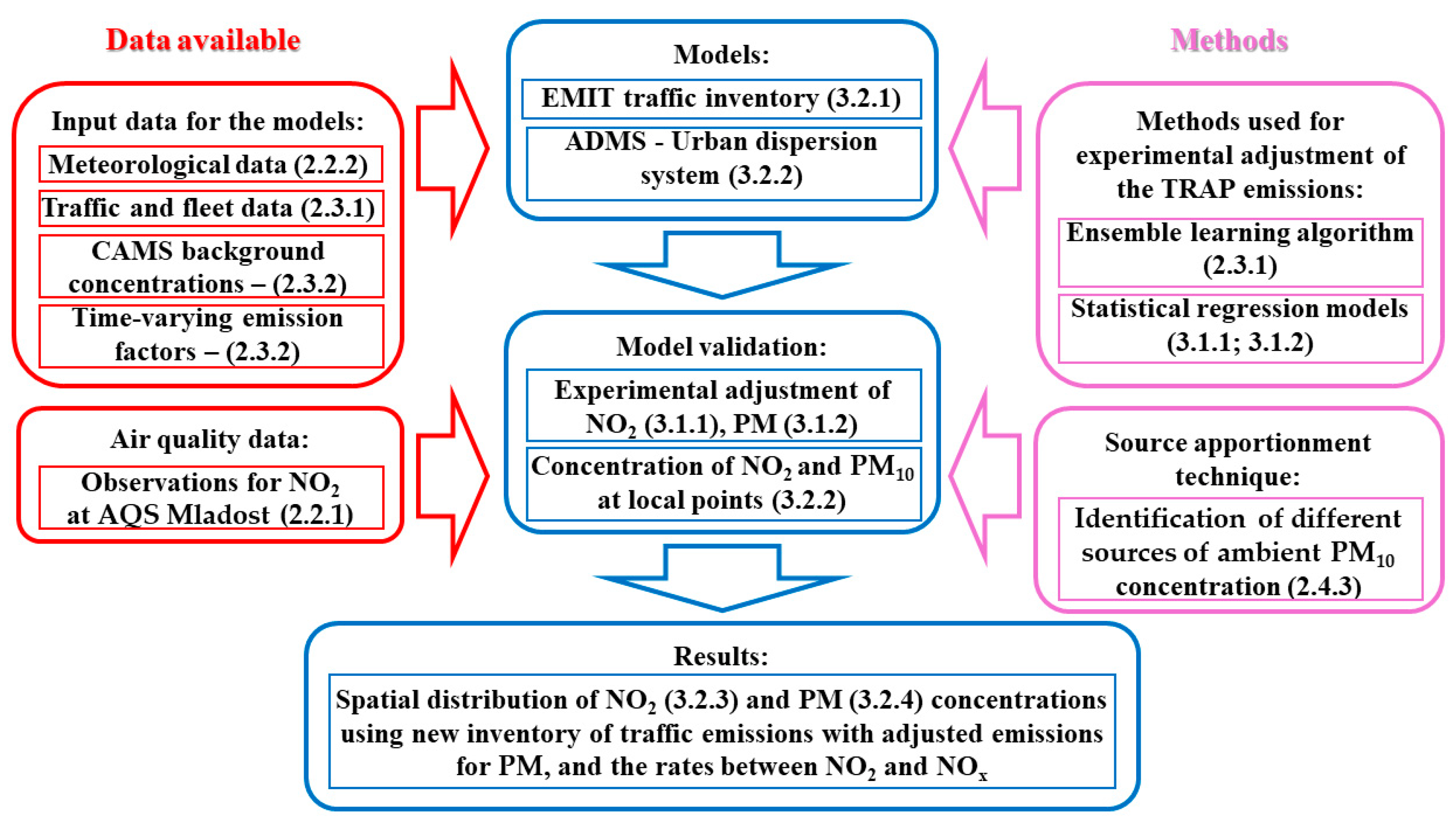
- To provide a means of adjusting the emissions of PM and the rates between NO2 and NOx gaseous pollutants, using hourly mean concentration measurements from road transport and urban background automatic air quality stations (AQSs) in Sofia, Bulgaria. Different already-published and new methods are explored and evaluated.
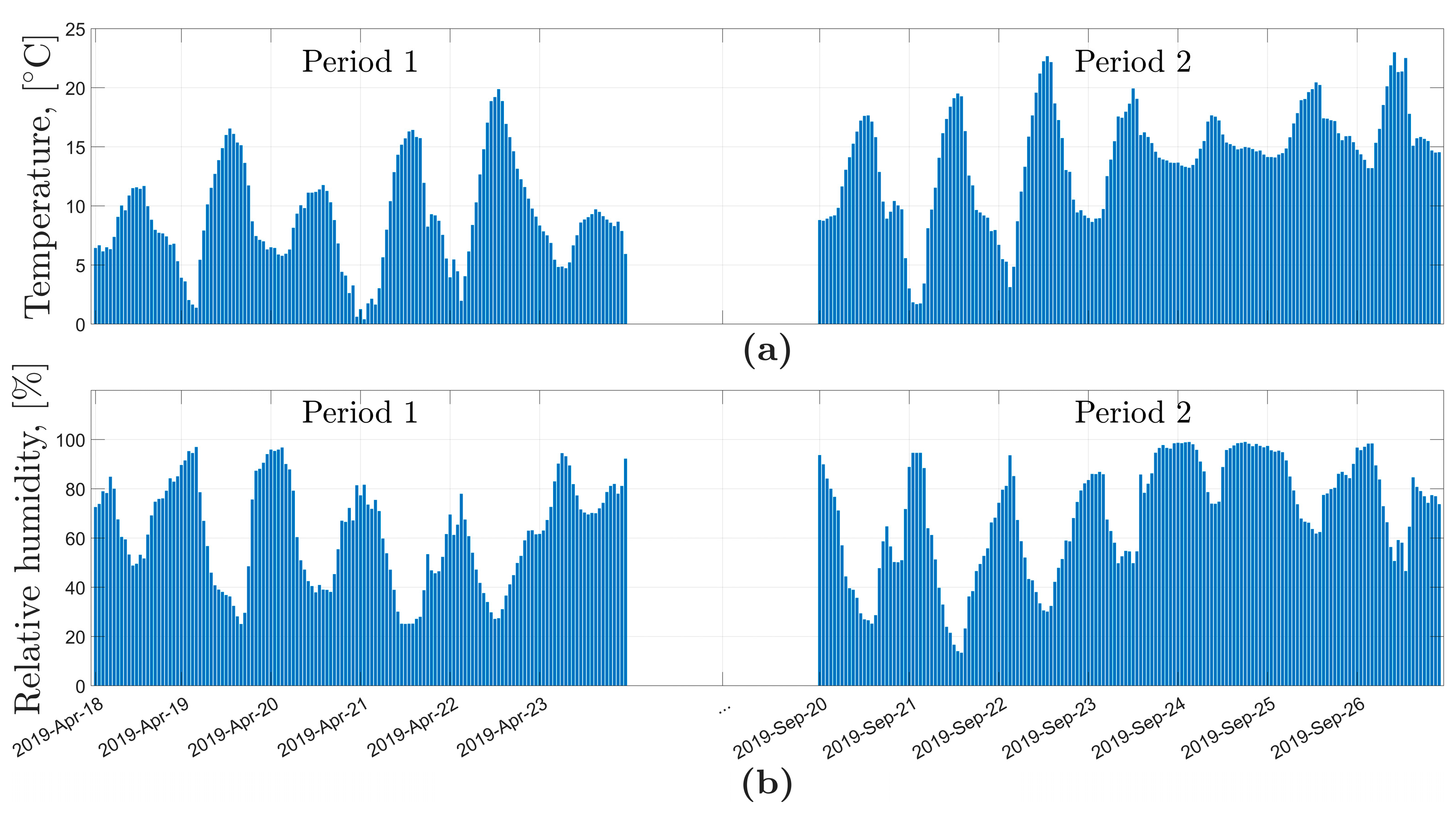
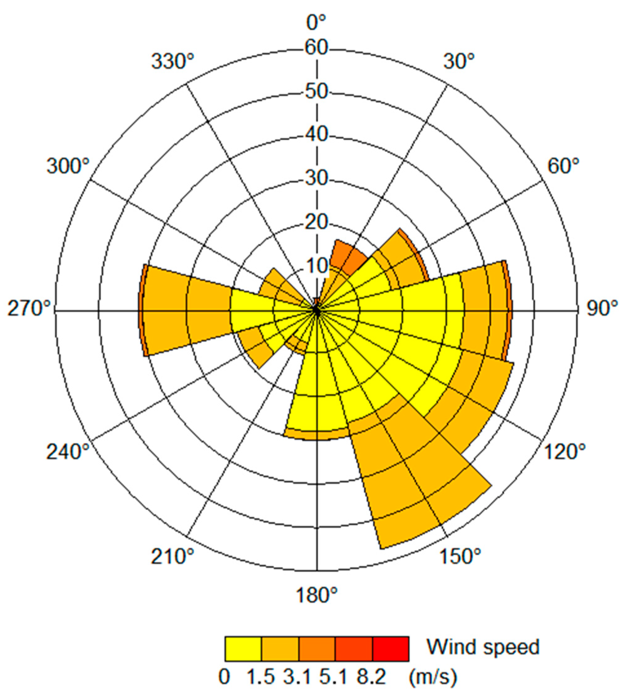
- To estimate the contribution of PM10 traffic emissions. To identify the contribution of the main groups of PM10 sources in Sofia, the results of a receptor-oriented positive matrix factorization (PMF) analysis for a wide variety of chemical elements [34] are presented. This study covers one year (2019–2020), but selected periods in April and September 2019 are used to validate the newly developed PM10 traffic emissions. These periods were chosen considering several important factors—the absence of domestic heating and additional background sources such as dust transport from the Sahara Desert, lack of precipitation and low wind speed.
2. Materials and Methods
2.1. Research Question and Hypothesis
2.2. Data
2.2.1. Air Quality Data
2.2.2. Meteorological Data
2.3. Modeling
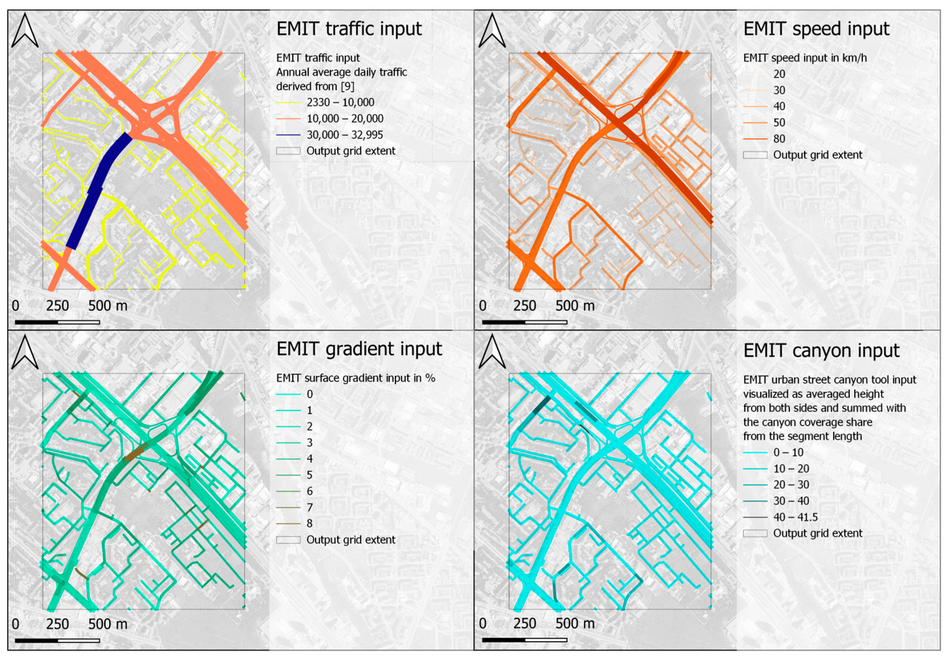
2.3.1. Transport Emission Inventory Modeling
2.3.2. Atmospheric Dispersion Modeling in Urban Street Canyons
2.4. Experimental Design of Emissions Adjustment
2.4.1. Study Approach for NO2 Concentration Adjustment
2.4.2. Study Approach for PM Emissions Adjustment
2.4.3. Source Apportionment Technique
3. Results
3.1. Results from Experimental Adjustment
3.1.1. Local NO2 Concentration Adjustment
3.1.2. Local PM Concentration Adjustment
3.2. Results from Modeling
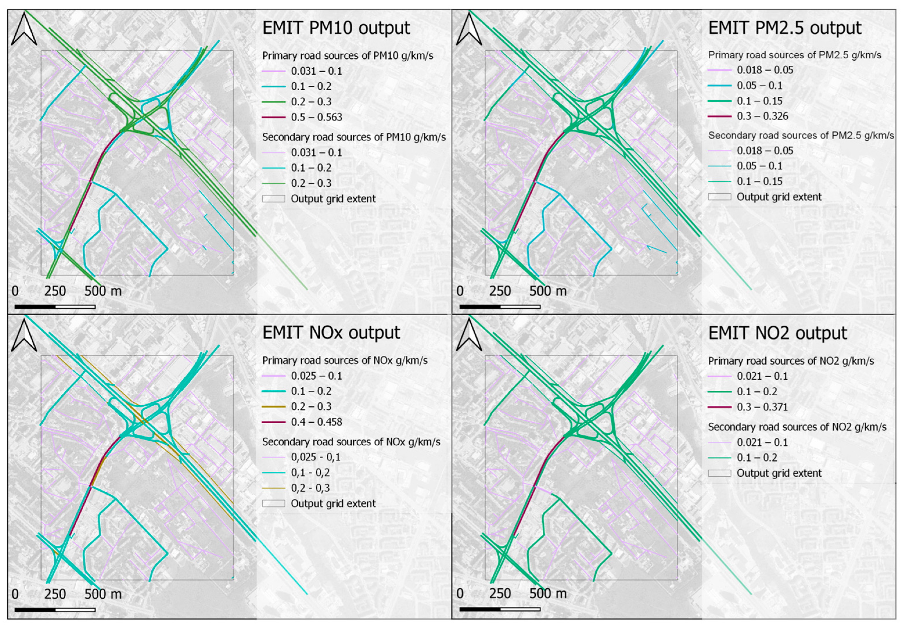
3.2.1. Transport Emission Inventory Modeling
3.2.2. ADMS-Urban Model Validation
Model Validation for NO2
Model Validation for PM10
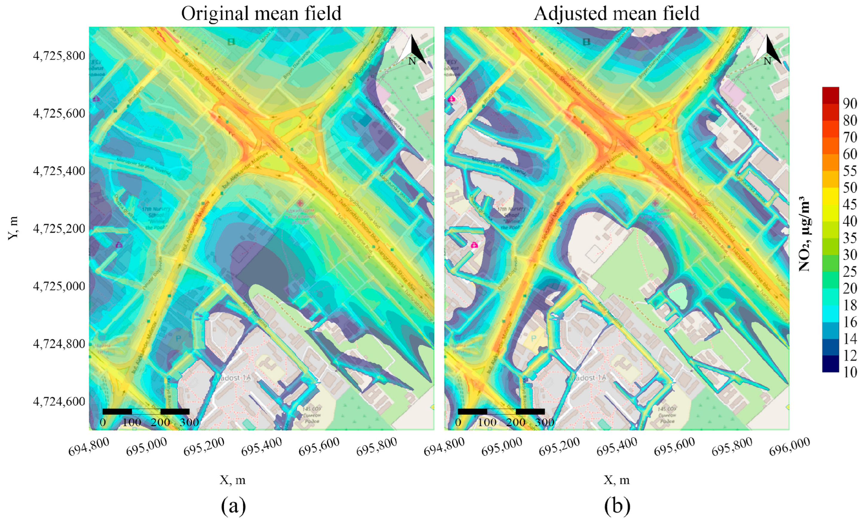
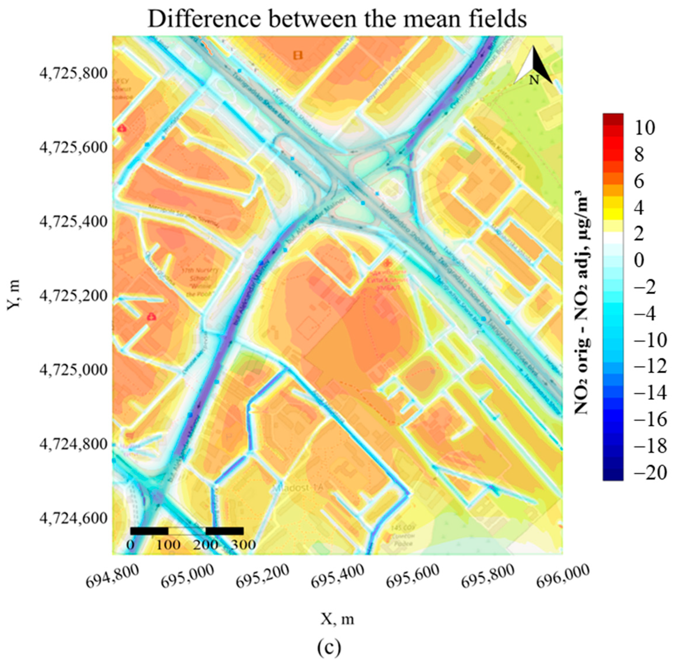
3.2.3. Spatial Distribution of NO2 Concentrations
3.2.4. Spatial Distribution of Concentrations of Different PM Fractions
4. Discussion
- The city of Sofia is the biggest urban area in the country, and despite the efforts made during the last few decades, the citizens in the capital are still exposed to high levels of PM10 as well as other pollutants, especially NO2. The latter is mostly related to traffic, but the evidence has somehow stayed hidden due to gaps in the monitoring of areas with more intensive traffic [26].
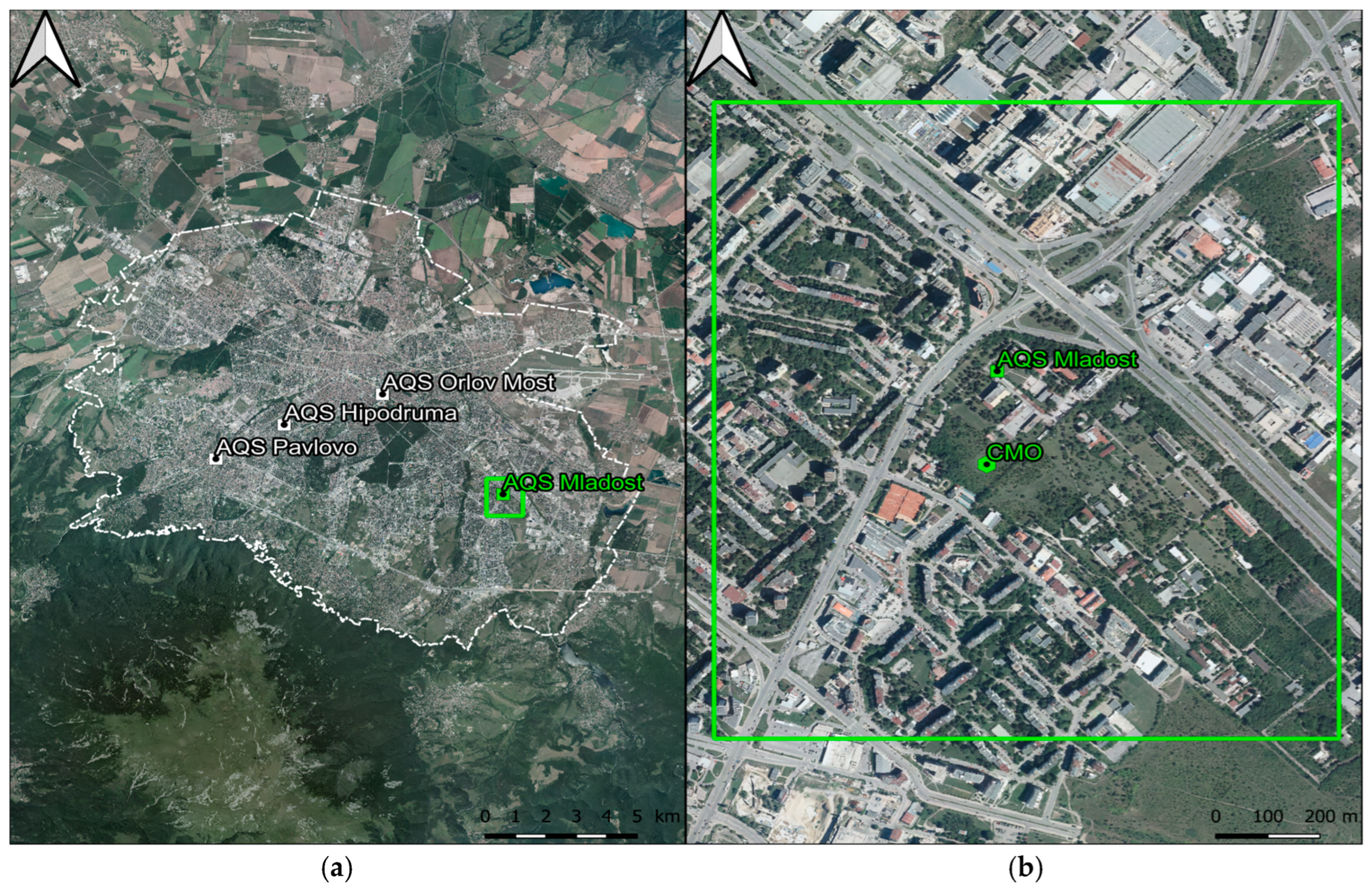
- Sofia as a study object is a challenging and complex urban system because of its geographical setting and due to the fast expansion of the city and the recent tendencies in compact and car-oriented urban development. Unfavorable in terms of air quality are the rising density and share of impervious surfaces, urban street canyon formation, and the interruption of “green wedges”, which have an important role in the ventilation of the city. In the previous two decades, investment priority was given to the construction of new transport infrastructure for untapping some “bottlenecks,” but this has induced demand, encouraging higher motorization and more intensive travel by private cars while increasing competition for the narrow space with the alternative mass or active mobility options [68,69,70].
- Despite the relative scarcity of reliable observational data, Sofia is well ahead in terms of experimental infrastructure in comparison to other cities in Bulgaria. Matching the different sources of data and information is a challenging endeavor in the pursuit of better knowledge, which can contribute to more appropriate decision-making.
5. Conclusions
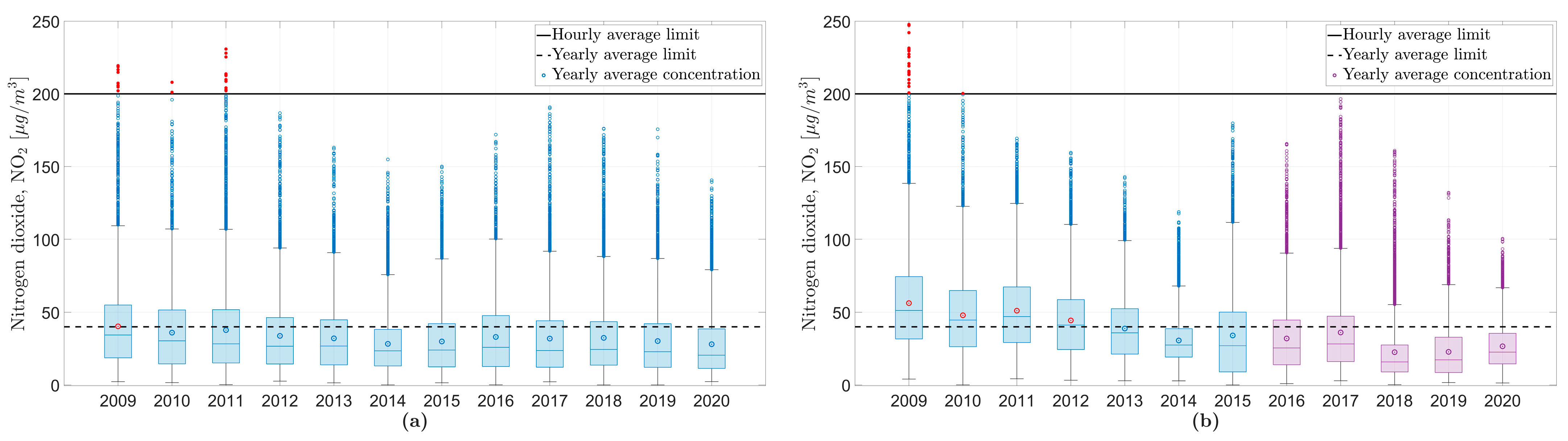
- Descriptive statistics based on observations at three transport stations in Sofia over an extended period (2009–2020) show a trend in the average annual concentrations of NO2 and PM10. A slightly negative trend (decrease in averaged annual concentration) was registered at AQS Pavlovo. The highest values were measured at AQS Orlov Most, but these decreased significantly after the station was moved to a new location in Mladost. The lowest recorded concentrations in 2019 and 2020 are most likely due to the imposed lockdown during the COVID-19 pandemic. Hourly concentrations of NO2 (averaged for the entire period) for weekdays, Saturday, and Sunday are also presented as evidence of the diurnal profiles of traffic-related emissions.
- A new inventory of traffic emissions has been developed for the city of Sofia based on publicly available traffic and fleet data, as well as a dedicated data collection campaign to fill the gaps in secondary street traffic data. Various processing steps were applied to align diverse geometry, attribute data, and acquisition methods, utilizing the advantages of ensemble learning. This activity data were used with the EMIT model to calculate the traffic emissions. The emissions were then exploited to simulate air pollution in a specific area by the ADMS-Urban model.
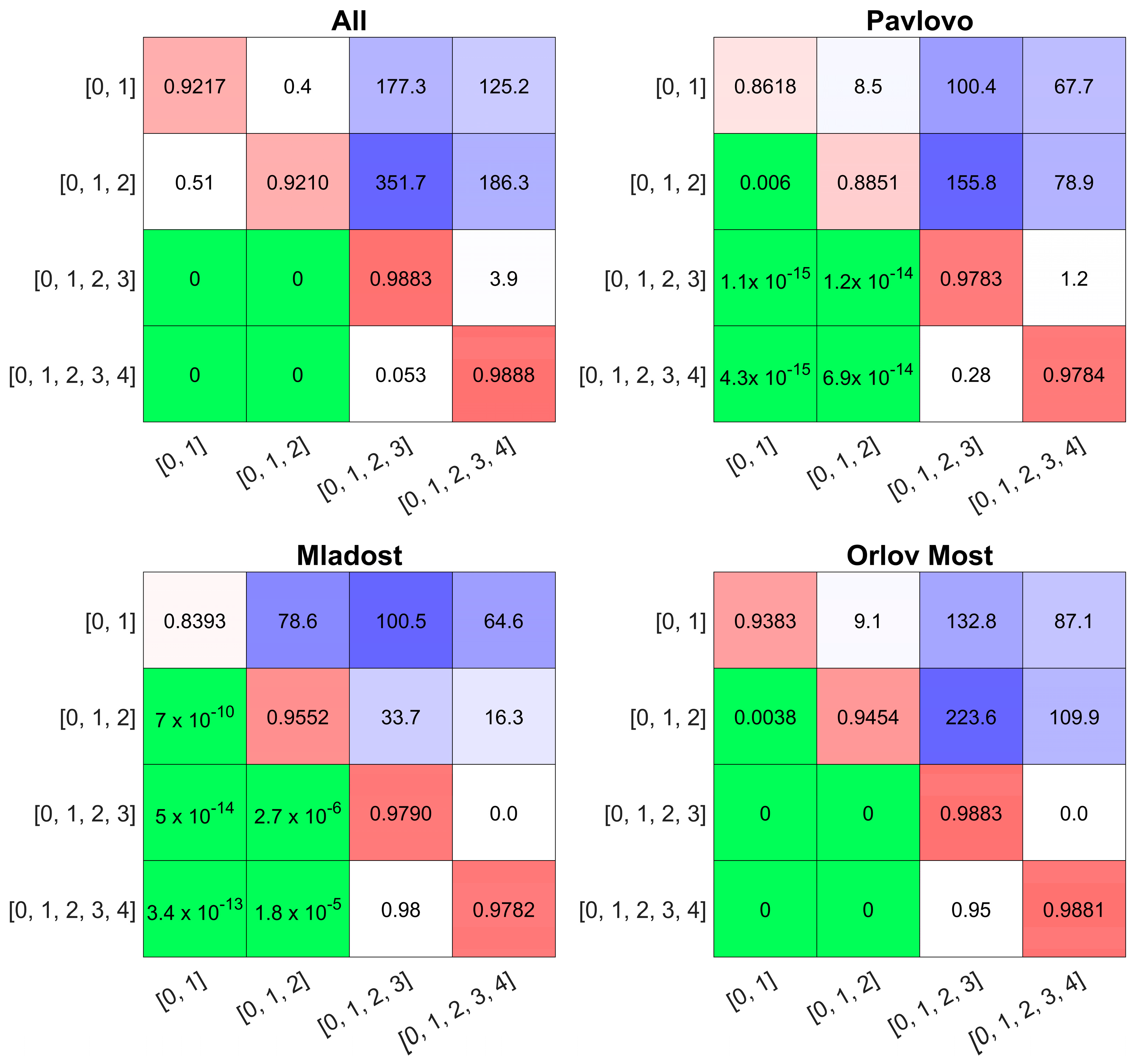
- The polynomial relationship between NOx and NO2 was adjusted based on local dynamics at three AQSs in Sofia for a 12-year period (from 2009 to 2020), to provide a more adequate estimation of NO2 from the ADMS-Urban model.
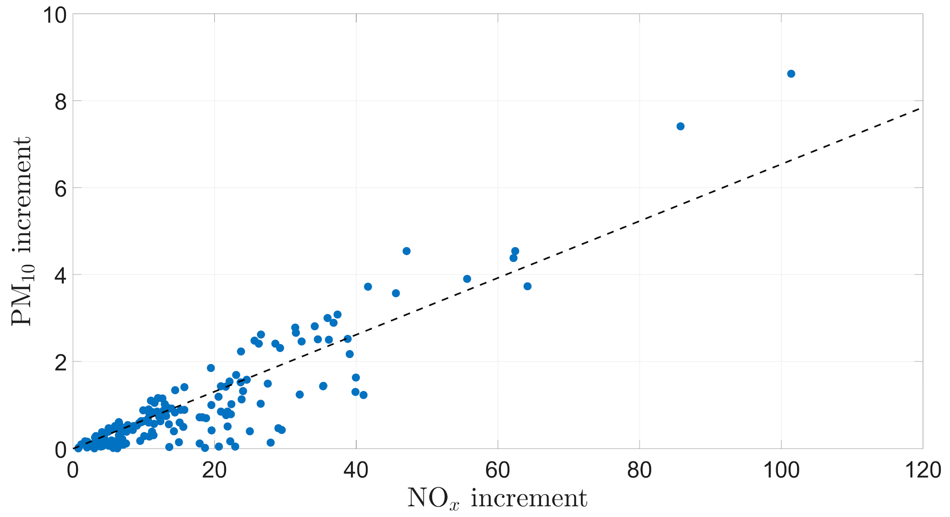
- Models of the first and second order with all interactions were fit to data for 12 measurands at AQS Hipodruma (where PM2.5 observations are available) for the period from 2015 to 2020. The two models were validated on one-year worth of data from 2023. Due to its better performance statistics, the second-order model was chosen to predict the concentration of PM2.5 at the chosen traffic station, AQS Pavlovo. Data from both transport and urban background stations were used to calculate the roadside increments and the adjusted emissions of PM10 and PMcoarse.
- The ADMS-Urban model was validated and evaluated by comparing pollutant concentrations from simulations using original and adjusted emissions, showing an improvement in results after applying functions and relationships derived from local observations.
Supplementary Materials
Author Contributions
Funding
Institutional Review Board Statement
Informed Consent Statement
Data Availability Statement
Acknowledgments
Conflicts of Interest
Abbreviations
| TRAP | Traffic-Related Air Pollution |
| PM | Particulate Matter |
| LPG | Liquefied Petroleum Gas |
| NOx | Nitrogen Oxides |
| EC | Elemental Carbon |
| PM2.5 | Particulate Matter Not Exceeding 2.5 μm in Aerodynamic Diameter |
| UFPs | Ultrafine Particles Not Exceeding 1 μm in Aerodynamic Diameter |
| PAH | Polycyclic Aromatic Hydrocarbons |
| VOC | Volatile Organic Compounds |
| PM10 | Particulate Matter Not Exceeding 10 μm in Aerodynamic Diameter () |
| THC | Total Hydrocarbons |
| CO | Carbon Monoxide |
| COPERT | European Computer Model to Calculate Emissions from Road Traffic |
| MOBILE | Mobile Source Emissions Factor Model |
| MOVES | Motor Vehicle Emission Simulator |
| HBEFA | Handbook Emission Factors for Road Transport |
| EMIT | Comprehensive Emissions Inventory Toolkit |
| CMEM | Comprehensive Modal Emission Model |
| ESTM | Multimodal Traffic Simulation Software |
| EMPA | Swiss Federal Laboratories for Materials Testing and Research |
| NAEI | UK National Atmospheric Emissions Inventory |
| NO2 | Nitrogen Dioxide |
| AQS | Automatic Air Quality Stations |
| ADMS-Urban | Air Quality Management & Assessment System |
| CERC | Cambridge Environmental Research Consultants Ltd. |
| O3 | Ozone |
| SO2 | Sulphur Dioxide |
| CAMS | Copernicus Atmosphere Monitoring Service |
| TNO | Netherlands Organization for Applied Scientific Research |
| CMO | Central Meteorological Observatory |
| EEA | Executive Environment Agency |
| EMEP | European Monitoring and Evaluation Programme |
| Defra/TRL | Department for Environment, Food and Rural Affairs/Transport Research Laboratory |
| RMSE | Root-Mean-Square Error |
| IA | Index of Agreement |
| SA | Source Apportionment |
| PMF | Positive Matrix Factorization |
| EPA | Environmental Protection Agency |
| RES | Resuspension |
| SEC | Secondary |
| BB | Biomass Burning |
| TR | Traffic |
| IND | Industry |
| FUEL | Fuel-Oil Burning |
| CO | Carbon Monoxide |
| NO | Nitrogen Monoxide |
| NMB | Normalized Mean Bias |
| NME | Normalized Mean Error |
References
- EUROSAT, Database—Transport—Eurostat—European Commission. Available online: https://ec.europa.eu/eurostat/web/transport/data/database (accessed on 13 May 2024).
- EUROSAT, Database—Transport—Eurostat—European Commission. Available online: https://ec.europa.eu/eurostat/web/products-eurostat-news/w/ddn-20240117-1 (accessed on 13 May 2024).
- Selleri, T.; Melas, A.D.; Joshi, A.; Manara, D.; Perujo, A.; Suarez-Bertoa, R. An Overview of Lean Exhaust deNOx Aftertreatment Technologies and NOx Emission Regulations in the European Union. Catalysts 2021, 11, 404. [Google Scholar] [CrossRef]
- Selleri, T.; Gioria, R.; Melas, A.D.; Giechaskiel, B.; Forloni, F.; Villafuerte, P.M.; Demuynck, J.; Bosteels, D.; Wilkes, T.; Simons, O.; et al. Measuring Emissions from a Demonstrator Heavy-Duty Diesel Vehicle under Real-World Conditions—Moving Forward to Euro VII. Catalysts 2022, 12, 184. [Google Scholar] [CrossRef]
- Frey, H.C. Trends in Onroad Transportation Energy and Emissions. J. Air Waste Manag. Assoc. 2018, 68, 514–563. [Google Scholar] [CrossRef]
- European Environmental Agency. National Emission Reduction Commitments Directive Emissions Inventory Data. 2024. Available online: https://www.eea.europa.eu/data-and-maps/dashboards/necd-directive-data-viewer-7 (accessed on 17 June 2024).
- Mehlhart, G.; Merz, C.; Akkermans, L.; Jordal-Jorgensen, J. European Second-Hand Car Market Analysis, Final Report. 2011. Available online: https://www.oeko.de/oekodoc/1114/2011-005-en.pdf (accessed on 13 May 2024).
- National Statistical Institute. Theme 7. SUSTAINABLE TRANSPORT: 7.6. Share of New Registered and Registered Brand New Vehicles. 2016. Available online: https://www.nsi.bg/sites/default/files/files/data/timeseries/SDI%207.6_en.xls (accessed on 17 June 2024).
- Burov, A.; Brezov, D. Transport Emissions from Sofia’s Streets—Inventory, Scenarios, and Exposure Setting. In Environmental Protection and Disaster Risks. EnviroRISKs 2022. Lecture Notes in Networks and Systems; Dobrinkova, N., Nikolov, O., Eds.; Springer: Cham, Switzerland, 2023; Volume 638, pp. 223–233. [Google Scholar] [CrossRef]
- Za Zemiata. Spatial-Based Scenarios for the Introduction of Low-Emission Zones for Transport in the Metropolitan Municipality Guidelines for Related Measures/Appendixes/. 2024. Available online: https://www.zazemiata.org/wp-content/uploads/2023/02/AirNEZ_web_landscape_FINALANNEXES_2024.pdf (accessed on 17 June 2024).
- Mądziel, M. Vehicle Emission Models and Traffic Simulators: A Review. Energies 2023, 16, 3941. [Google Scholar] [CrossRef]
- Zhang, R.; Wang, Y.; Pang, Y.; Zhang, B.; Wei, Y.; Wang, M.; Zhu, R. A Deep Learning Micro-Scale Model to Estimate the CO2 Emissions from Light-Duty Diesel Trucks Based on Real-World Driving. Atmosphere 2022, 13, 1466. [Google Scholar] [CrossRef]
- De Nunzio, G.; Laraki, M.; Thibault, L. Road Traffic Dynamic Pollutant Emissions Estimation: From Macroscopic Road Information to Microscopic Environmental Impact. Atmosphere 2021, 12, 53. [Google Scholar] [CrossRef]
- COPERT Computer Model to Calculate Emissions from Road Traffic. Available online: https://web.jrc.ec.europa.eu/policy-model-inventory/explore/models/model-copert (accessed on 8 March 2024).
- Description and History of the MOBILE Highway Vehicle Emission Factor Model. Available online: https://www.epa.gov/moves/description-and-history-mobile-highway-vehicle-emission-factor-model (accessed on 8 March 2024).
- The Handbook of Emission Factors for Road Transport (HBEFA). Available online: https://www.hbefa.net (accessed on 8 March 2024).
- Cambridge Environmental Research Consultants Ltd. Atmospheric Emissions Inventory Toolkit (EMIT). Version 3.9. User Guide. 2022. Available online: https://www.cerc.co.uk/environmental-software/assets/data/doc_userguides/CERC_EMIT3.9_User%20Guide.pdf (accessed on 8 March 2024).
- Mao, F.; Li, Z.; Zhang, K. A Comparison of Carbon Dioxide Emissions between Battery Electric Buses and Conventional Diesel Buses. Sustainability 2021, 13, 5170. [Google Scholar] [CrossRef]
- Comprehensive Modal Emission Model (CMEM). Available online: https://www.cert.ucr.edu/cmem (accessed on 8 March 2024).
- Environmentally Sensitive Traffic Management (ESTM). Available online: https://www.bosch-mobility.com/en/solutions/air-quality-solutions/environmentally-sensitive-traffic-management (accessed on 8 March 2024).
- Swiss Federal Laboratories for Materials Testing and Research (EMPA), Future Mobility. Available online: https://www.empa.ch/web/empa/future-indiviual-mobility (accessed on 8 March 2024).
- West, J.L.; Mobley, J.D.; Deslauriers, M.; Feldman, H.; Frey, C.; Rojas-Bracho, L.; Wierman, S.S.; Werner, A.S. NARSTO emission inventory assessment. In Proceedings of the American Association of Aerosol Research 2005, Atlanta, GA, USA, 7–11 February 2005. [Google Scholar]
- Health Effects Institute. Panel on the Health Effects of Traffic-Related Air Pollution. In Traffic-Related Air Pollution: A Critical Review of the Literature on Emissions, Exposure, and Health Effects; HEI Special Report 17; Health Effects Institute: Boston, MA, USA, 2010. [Google Scholar]
- Thorpe, A.; Harrison, R.M. Sources and properties of non-exhaust particulate matter from road traffic: A review. Sci. Total Environ. 2008, 400, 270–282. [Google Scholar] [CrossRef]
- Boulter, P.G.; Thorpe, A.J.; Harrison, R.M.; Allen, A.G. Road Vehicle Non-Exhaust Particulate Matter: Final Report on Emission Modelling, CPEA23/SPU82 Project Report. 2007. Available online: https://uk-air.defra.gov.uk/assets/documents/reports/cat15/0706061624_Report2_Emission_modelling.PDF (accessed on 8 March 2024).
- Executive Environment Agency, System for Informing the Population about the Quality of Atmospheric Air. Available online: https://eea.government.bg/kav (accessed on 8 March 2024). (In Bulgarian)
- Executive Environment Agency. National Report for the Condition and Preservation of the Environment: Pollutant Emissions and Quality of the Atmospheric Air. 2023. Available online: https://eea.government.bg/bg/soer/2023/1Air.pdf (accessed on 8 March 2024). (In Bulgarian)
- AIRTHINGS—A Pilot System of Sensors for Monitoring Atmospheric Air. Available online: https://air.sofia.bg (accessed on 8 March 2024). (In Bulgarian).
- Network of Low-Cost Citizen-Owned Sensor Suites. Available online: https://airsofia.info (accessed on 8 March 2024). (In Bulgarian).
- European Clean Air Centre. State of Air Quality in Bulgaria: Overview. 2020. Available online: https://cleanaircentre.eu/wp-content/uploads/2019/10/State-of-AQ-Bulgaria.pdf (accessed on 8 March 2024).
- Popov, I.; Hlebarov, I.; Raeva, D. Is There Nitrogen Dioxide Pollution of the Air in Sofia? 2022. Available online: https://www.zazemiata.org/wp-content/uploads/2022/05/Za-Zemyata-Doklad-NO2-Online.pdf (accessed on 8 March 2024). (In Bulgarian).
- Zareba, M.; Weglinska, E.; Danek, T. Air pollution seasons in urban moderate climate areas through big data analytics. Sci. Rep. 2024, 14, 3058. [Google Scholar] [CrossRef] [PubMed]
- Health Effects Institute. Trends in Air Quality and Health in Southeast Europe: A State of Global Air Special Report; Health Effects Institute: Boston, MA, USA, 2022; ISSN 2578-6881; Available online: https://www.stateofglobalair.org/sites/default/files/documents/2022-05/soga-southeast-europe-regional-report_1.pdf (accessed on 17 June 2024).
- Hristova, E.; Veleva, B.; Georgieva, E.; Branzov, H. Application of Positive Matrix Factorization Receptor Model for Source Identification of PM10 in the City of Sofia, Bulgaria. Atmosphere 2020, 11, 890. [Google Scholar] [CrossRef]
- Air Quality: Commission Decides to Refer Bulgaria to the Court of Justice over Its Failure to Comply with Previous Judgement. Available online: https://ec.europa.eu/commission/presscorner/detail/en/ip_20_2150 (accessed on 8 March 2024).
- Stefanov, B.; Dombalov, I.; Pelovski, Y.; Kozarev, N.; Ilieva, N.; Sokolovski, E.; Borisov, D.; Nikolova, Y.; Georgieva, A.; Angelova, S.; et al. Atmospheric Air Quality Management Program of Sofia Municipality for the Period 2015–2020—Reduction of Emissions and Reach of the Established Norms for Fine Particles PM10. 2015. Available online: https://www.sofia.bg/documents/20121/129306/Project_Program_KAV_Sofia_2015-2020.pdf (accessed on 8 March 2024). (In Bulgarian).
- Kozarev, N.; Dombalov, I.; Sokolovski, E.; Ilieva, N.; Predyov, I. Program for Supplementation of the Program “Atmospheric air Quality Management Program of Capital Municipality for the Period 2015–2020—Reduction of Emissions and Achievement of the Established Norms for Fine Particles PM10”, by Indicators of Fine Particles with Size up to 2.5 Microns and Polycyclic Aromatic Hydrocarbons. 2019. Available online: https://air.sofia.bg/media/Documents/R.523-Pr1.pdf (accessed on 8 March 2024). (In Bulgarian).
- Sofia Municipality. Program for Improving the Air Quality on the Territory of Sofia Municipality for the Period 2021–2026. 2019. Available online: https://www.sofia.bg/documents/20121/992246/Пpoeкт+нa+Пpoгpaмa+KAB+2021-2026.pdf/ (accessed on 8 March 2024). (In Bulgarian).
- Dimitrova, R.; Velizarova, M. Assessment of the contribution of different particulate matter sources on pollution in Sofia City. Atmosphere 2021, 12, 423. [Google Scholar] [CrossRef]
- Brezov, D.; Burov, A. Ensemble Learning Traffic Model for Sofia: A Case Study. Appl. Sci. 2023, 13, 4678. [Google Scholar] [CrossRef]
- Carruthers, D.J.; Edmunds, H.A.; McHugh, C.A.; Singles, R.J. Development of ADMS-Urban and Comparison with Data for Urban Areas in the UK. In Air Pollution Modeling and Its Application XII. NATO—Challenges of Modern Society; Gryning, S.E., Chaumerliac, N., Eds.; Springer: Boston, MA, USA, 1998; p. 22. [Google Scholar] [CrossRef]
- Stocker, J.; Hood, C.; Carruthers, D.; McHugh, C. ADMS-Urban: Developments in modelling dispersion from the city scale to the local scale. Int. J. Environ. Pollut. 2012, 50, 308–316. [Google Scholar] [CrossRef]
- Georgieva, E.; Syrakov, D.; Prodanova, M.; Etropolska, I.; Slavov, K. Evaluating the performance of WRF-CMAQ air quality modelling system in Bulgaria by means of the DELTA tool. Int. J. Environ. Pollut. 2015, 57, 272. [Google Scholar] [CrossRef]
- Average Age of Registered Passenger Cars in Selected European Countries as of 2019. Available online: https://www.statista.com/statistics/974713/passenger-car-average-age-europe/ (accessed on 25 July 2023).
- Carslaw, D.C.; Rhys-Tyler, G. New insights from comprehensive on-road measurements of NOx, NO2 and NH3from vehicle emission remote sensing in London, UK. Atmos. Environ. 2013, 81, 339–347. [Google Scholar] [CrossRef]
- Regulation 12 of 15 July 2010 for the Limit Levels of Sulphur Dioxide, Nitrous Dioxide, Fine Particulate Matter, Lead, Benzene, Carbon Monoxide and Ozone in the Atmosphere. Available online: https://lex.bg/bg/laws/ldoc/2135691821 (accessed on 12 February 2024). (In Bulgarian).
- VAISALA Product Documentation Portal. Available online: https://docs.vaisala.com/v/u/B211729EN-E/en-US (accessed on 8 March 2024).
- VAISALA Product Documentation Portal. Available online: https://docs.vaisala.com/v/u/B211221EN-L/en-US (accessed on 8 March 2024).
- VAISALA Product Documentation Portal. Available online: https://docs.vaisala.com/v/u/B212709EN-A/en-US (accessed on 8 March 2024).
- UK National Atmospheric Emissions Inventory (NAEI). Available online: https://naei.beis.gov.uk/about (accessed on 8 March 2024).
- The Co-Operative Programme for Monitoring and Evaluation of the Long-Range Transmission of Air Pollutants in Europe (EMEP). Available online: https://www.emep.int (accessed on 8 March 2024).
- Cambridge Environmental Research Consultants Ltd. ADMS-Urban. Urban Air Quality Management System. Version 5.0. User Guide. 2020. Available online: https://www.cerc.co.uk/environmental-software/assets/data/doc_userguides/CERCADMS-Urban5.0_User_Guide.pdf (accessed on 25 July 2023).
- Venkatram, A.; Karamchandani, P.; Pai, P.; Goldstein, R. The development and application of a simplified ozone modeling system (SOMS). Atmos. Environ. 1994, 28, 3665–3678. [Google Scholar] [CrossRef]
- Copernicus Atmosphere Monitoring Service. Available online: https://atmosphere.copernicus.eu (accessed on 8 March 2024).
- Cambridge Environmental Research Consultants Ltd. ADMS Street Canyon Tool. Version 2.0. User Guide. 2018. Available online: https://www.cerc.co.uk/environmental-software/assets/data/doc_userguides/CERC_Street_Canyon_Tool_User_Guide.pdf (accessed on 8 March 2024).
- Builtjes, P.J.H.; van Loon, M.; Schaap, M.; Teeuwisse, S.; Visschedijk, A.J.H.; Bloos, J.P. Project on the Modelling and Verification of Ozone Reduction Strategies: Contribution of TNO-MEP, TNO-Report, MEP-R2003/166; Netherlands Environmental Assessment Agency: Apeldoorn, The Netherlands, 2003. [Google Scholar]
- Technical Specification Documents. Available online: https://www.cerc.co.uk/environmental-software/technical-specifications.html (accessed on 8 March 2024).
- Derwent, R.G.; Middleton, D.R. An empirical function for the ratio [NO2]:[NOx]. Clean Air 1996, 26, 57–60. [Google Scholar]
- Dixon, J.; Middleton, D.R.; Derwent, R.G. Sensitivity of nitrogen dioxide concentrations to oxides of nitrogen controls in the United Kingdom. Atmos. Environ. 2001, 35, 3715–3728. [Google Scholar] [CrossRef]
- Neto, E.d.A.L.; de Carvalho, F.d.A.T. Constrained linear regression models for symbolic interval-valued variables. Comput. Stat. Data Anal. 2010, 54, 333–347. [Google Scholar] [CrossRef]
- Harrison, R.M.; Yin, J.; Mark, D.; Stedman, J.; Appleby, R.S.; Booker, J.; Moorcroft, S. Studies of the coarse particle (2.5–10 µm) component in UK urban atmospheres. Atmos. Environ. 2001, 35, 3667–3679. [Google Scholar] [CrossRef]
- Harrison, R.M.; Jones, A.M.; Barrowcliffe, R. Field study of the influence of meteorological factors and traffic volumes upon suspended particle mass at urban roadside sites of differing geometries. Atmos. Environ. 2004, 38, 6361–6369. [Google Scholar] [CrossRef]
- Grigoratos, T.; Martini, G. Brake wear particle emissions: A review. Environ. Sci. Pollut. Res. 2015, 22, 2491–2504. [Google Scholar] [CrossRef] [PubMed]
- Amato, F.; Pandolfi, M.; Viana, M.; Querol, X.; Alastuey, A.; Moreno, T. Spatial and chemical patterns of PM10 in road dust deposited in urban environment. Atmos. Environ. 2009, 43, 1650–1659. [Google Scholar] [CrossRef]
- Denby, B.R.; Kupiainen, K.J.; Gustafsson, M. Chapter 9—Review of road dust emissions. In Non-Exhaust Emissions; Amato, F., Ed.; Academic Press: Cambridge, MA, USA, 2018; pp. 183–203. [Google Scholar]
- Norris, G.; Duvall, R.; Brown, S.; Bai, S. EPA Positive Matrix Factorization (PMF) 5.0 Fundamentals and User Guide. 2014. Available online: https://www.epa.gov/sites/default/files/2015-2/documents/pmf_5.0_user_guide.pdf (accessed on 26 September 2021).
- Mircea, M.; Calori, G.; Pirovano, G.; Belis, C. European Guide on air Pollution Source Apportionment for Particulate Matter with Source-Oriented Models and Their Combined Use with Receptor Models; Publications Office of the European Union: Luxembourg, 2020. [Google Scholar] [CrossRef]
- Madzhirski, V.; Dimitrova, E. Challenges and Lessons Learned during the Initial Implementation of EU Urban Mobility Policy in Bulgarian Cities in the period 2007–2017. Corvinus Reg. Stud. 2019, 4, 83–97. [Google Scholar]
- Sustainable Urban Mobility Plan of Sofia. 2019. Available online: https://sofiaplan.bg/wp-content/uploads/2022/05/SUMP-21-05-2019.pdf (accessed on 13 May 2024).
- Program for Sofia, I_Territorial Scope and Analysis of the State. 2021. Available online: https://sofiaplan.bg/wp-content/uploads/2021/09/I_Tepитopиaлeн-oбхвaт-и-aнaлиз-нa-състoяниeтo-2.pdf (accessed on 13 May 2024).
- Mensah, G.A.; Fuster, V.; Murray, C.J.L.; Roth, G.A. Global Burden of Cardiovascular Diseases and Risks, 1990–2022. J. Am. Coll. Cardiol. 2023, 82, 2350–2473. [Google Scholar] [CrossRef]
- Health Effects Institute. Trends in Air Quality and Health in Bulgaria: A State of Global Air Special Report. Boston, MA, 2020. Available online: https://www.stateofglobalair.org/sites/default/files/documents/2022-06/soga-southeast-europe-bulgaria-report.pdf (accessed on 5 January 2024).
- World Health Organization. WHO global Air Quality Guidelines: Particulate Matter (PM2.5 and PM10), Ozone, Nitrogen Dioxide, Sulphur Sulfur Dioxide and Carbon Monoxide. Executive Summary. Geneva: World Health Organization. Available online: https://iris.who.int/handle/10665/345334 (accessed on 13 May 2024).
- Directive 2008/50/EC of the European Parliament and of the Council of 21 May 2008 on Ambient Air Quality and Cleaner Air for Europe; Annex III, Section C: Microscale Siting of Sampling Points. Available online: https://eur-lex.europa.eu/eli/dir/2008/50/oj (accessed on 13 May 2024).


| All Stations | Pavlovo | Mladost | Orlov Most | |||||
|---|---|---|---|---|---|---|---|---|
| Active Terms | R2 adj. | AIC | R2 adj. | AIC | R2 adj. | AIC | R2 adj. | AIC |
| [0, 1] | 0.92 | −249.4 | 0.86 | −130.6 | 0.84 | −102.8 | 0.94 | −268.2 |
| [0, 1, 2] | 0.92 | −247.9 | 0.89 | −136.8 | 0.96 | −142.7 | 0.95 | −275.0 |
| [0, 2] | 0.91 | −242.6 | 0.89 | −138.0 | 0.90 | −119.1 | 0.90 | −238.9 |
| [0, 1, 2, 3] | 0.99 | −369.1 | 0.98 | −201.0 | 0.98 | −166.0 | 0.99 | −372.4 |
| [0, 2, 3] | 0.93 | −257.2 | 0.88 | −136.0 | 0.94 | −135.0 | 0.96 | −296.1 |
| [0, 1, 3] | 0.92 | −247.4 | 0.88 | −134.5 | 0.95 | −137.2 | 0.95 | −279.0 |
| [0, 3] | 0.88 | −220.1 | 0.88 | −134.9 | 0.93 | −131.1 | 0.85 | −209.9 |
| [0, 1, 2, 3, 4] | 0.99 | −371.2 | 0.98 | −200.3 | 0.98 | −164.0 | 0.99 | −370.4 |
| [0, 2, 3, 4] | 0.98 | −348.4 | 0.98 | −201.0 | 0.98 | −164.5 | 0.99 | −367.4 |
| [0, 1, 3, 4] | 0.99 | −355.9 | 0.98 | −202.2 | 0.98 | −165.4 | 0.99 | −369.5 |
| [0, 1, 2, 4] | 0.99 | −363.7 | 0.98 | −202.1 | 0.98 | −165.9 | 0.99 | −371.8 |
| [0, 3, 4] | 0.95 | −276.7 | 0.89 | −140.2 | 0.94 | −132.0 | 0.98 | −329.3 |
| [0, 2, 4] | 0.94 | −262.2 | 0.88 | −136.2 | 0.94 | −132.0 | 0.97 | −306.6 |
| [0, 1, 4] | 0.92 | −247.6 | 0.87 | −132.6 | 0.94 | −132.4 | 0.95 | −283.2 |
| [0, 4] | 0.83 | −198.6 | 0.85 | −126.5 | 0.94 | −134.0 | 0.78 | −188.2 |
| Air Quality Monitoring Site | According to [59] (Yield) | This Study (Yield) | According to [58] (NO2) | This Study (NO2) |
|---|---|---|---|---|
| All stations | 10.9 | 0.013 | 8457.2 | 6.0 |
| Pavlovo | 5.4 | 0.018 | 3476.4 | 4.5 |
| Orlov Most | 10.9 | 0.013 | 8457.5 | 6.0 |
| Model | Number of Terms | Adjusted R2 | RMSE Training | RMSE Test |
|---|---|---|---|---|
| First-order | 13 | 0.862 | 10.5 µg/m3 | 8.29 µg/m3 |
| Second-order | 91 | 0.923 | 7.84 µg/m3 | 6.20 µg/m3 |
| Year | ||
|---|---|---|
| 2015 | 0.34 | 0.38 |
| 2016 | 0.35 | 0.46 |
| 2017 | 0.29 | 0.33 |
| 2018 | 0.32 | 0.33 |
| 2019 | 0.36 | 0.45 |
| 2020 | 0.38 | 0.47 |
| Date | AQS Mladost (Measured) | ADMS- Urban (Original) | ADMS- Urban (Adjusted) | Bias (Original) | Bias (Adjusted) | Error (Original) | Error (Adjusted) |
|---|---|---|---|---|---|---|---|
| 18 April2019 | 14.89 | 20.81 | 17.06 | 5.91 | 2.17 | 5.91 | 2.17 |
| 19 April 2019 | 13.81 | 32.24 | 10.49 | 18.43 | −3.32 | 18.43 | 3.32 |
| 20 April 2019 | 12.42 | 40.08 | 5.26 | 27.66 | −7.15 | 27.66 | 7.15 |
| 21 April 2019 | 8.01 | 26.66 | 4.40 | 18.65 | −3.61 | 18.65 | 3.61 |
| 22 April 2019 | 7.96 | 17.04 | 3.79 | 9.09 | −4.17 | 9.09 | 4.17 |
| 23 April 2019 | 8.34 | 15.09 | 14.04 | 6.75 | 5.70 | 6.75 | 5.70 |
| 20 September 2019 | 34.94 | 9.14 | 11.17 | −25.79 | −23.77 | 25.79 | 23.77 |
| 21 September 2019 | 30.15 | 8.46 | 3.76 | −21.69 | −26.39 | 21.69 | 26.39 |
| 22 September 2019 | 29.82 | 9.12 | 10.60 | −20.69 | −19.22 | 20.69 | 19.22 |
| 23 September 2019 | 45.33 | 19.70 | 24.13 | −25.63 | −21.20 | 25.63 | 21.20 |
| 24 September 2019 | 43.82 | 15.72 | 31.66 | −28.10 | −12.16 | 28.10 | 12.16 |
| 25 September 2019 | 40.89 | 8.51 | 18.82 | −32.38 | −22.07 | 32.38 | 22.07 |
| 26 September 2019 | 39.09 | 16.92 | 11.42 | −22.16 | −27.66 | 22.16 | 27.66 |
| Average | 25.34 | 18.42 | 12.81 | −6.92 | −12.53 | 20.23 | 13.74 |
| Date | PM10 (PMF) | PM10 (meas) | RES | TR | BB | IND | FUEL | N | SO4 | SEC |
|---|---|---|---|---|---|---|---|---|---|---|
| 18 April 2019 | 20.38 | 15.23 | 5.14 | 3.28 | 6.49 | 0.05 | 0.25 | 0.00 | 4.93 | 0.37 |
| 19 April 2019 | 21.41 | 17.58 | 4.91 | 3.87 | 4.67 | 0.11 | 0.24 | 0.00 | 2.80 | 4.84 |
| 20 April 2019 | 18.44 | 18.97 | 3.54 | 2.31 | 6.96 | 0.00 | 0.24 | 0.00 | 0.71 | 4.99 |
| 21 April 2019 | 19.59 | 20.66 | 6.26 | 2.32 | 4.22 | 0.68 | 0.19 | 0.00 | 0.00 | 7.08 |
| 22 April 2019 | 27.13 | 24.16 | 6.83 | 3.57 | 5.16 | 1.44 | 0.31 | 0.00 | 3.07 | 6.79 |
| 23 April 2019 | 28.63 | 27.55 | 3.34 | 3.31 | 9.40 | 2.18 | 0.22 | 0.17 | 6.87 | 3.13 |
| 20 September 2019 | 19.17 | 21.82 | 6.94 | 2.08 | 1.41 | 0.08 | 0.22 | 0.30 | 2.79 | 5.34 |
| 21 September 2019 | 19.20 | 24.06 | 5.93 | 2.68 | 4.09 | 0.15 | 0.16 | 0.07 | 6.08 | 0.04 |
| 22 September 2019 | 25.73 | 28.00 | 4.17 | 2.32 | 5.34 | 2.58 | 0.21 | 0.02 | 9.95 | 1.15 |
| 23 September 2019 | 29.91 | 32.42 | 7.84 | 4.84 | 4.04 | 1.09 | 0.03 | 0.28 | 9.57 | 2.20 |
| 24 September 2019 | 27.73 | 33.88 | 2.80 | 3.84 | 7.74 | 2.27 | 0.02 | 0.00 | 6.18 | 5.12 |
| 25 September 2019 | 29.73 | 30.79 | 2.90 | 3.28 | 2.80 | 2.00 | 0.05 | 0.00 | 12.08 | 6.74 |
| 26 September 2019 | 19.67 | 22.54 | 2.82 | 1.26 | 0.00 | 0.43 | 0.14 | 0.12 | 10.15 | 6.13 |
| Date | PMF Model at CMO | ADMS- Urban (Original) | ADMS- Urban (Adjusted) | Bias (Original) | Bias (Adjusted) | Error (Original) | Error (Adjusted) |
|---|---|---|---|---|---|---|---|
| 18 April2019 | 8.42 | 8.86 | 9.04 | 0.43 | 0.62 | 0.43 | 0.62 |
| 19 April 2019 | 8.78 | 8.13 | 8.24 | −0.65 | −0.55 | 0.65 | 0.55 |
| 20 April 2019 | 5.85 | 8.01 | 8.06 | 2.16 | 2.22 | 2.16 | 2.22 |
| 21 April 2019 | 8.57 | 5.83 | 5.87 | −2.75 | −2.70 | 2.75 | 2.70 |
| 22 April 2019 | 10.40 | 5.85 | 5.89 | −4.55 | −4.51 | 4.55 | 4.51 |
| 23 April 2019 | 6.65 | 6.56 | 6.63 | −0.09 | −0.02 | 0.09 | 0.02 |
| 20 September 2019 | 9.02 | 4.97 | 5.20 | −4.05 | −3.82 | 4.05 | 3.82 |
| 21 September 2019 | 8.61 | 5.37 | 5.28 | −3.24 | −3.33 | 3.24 | 3.33 |
| 22 September 2019 | 6.49 | 7.92 | 7.87 | 1.43 | 1.38 | 1.43 | 1.38 |
| 23 September 2019 | 12.68 | 6.44 | 6.19 | −6.24 | −6.49 | 6.24 | 6.49 |
| 24 September 2019 | 6.64 | 7.51 | 7.35 | 0.87 | 0.71 | 0.87 | 0.71 |
| 25 September 2019 | 6.18 | 6.59 | 6.42 | 0.42 | 0.24 | 0.42 | 0.24 |
| 26 September 2019 | 4.07 | 6.74 | 6.72 | 2.67 | 2.65 | 2.67 | 2.65 |
| Average | 7.87 | 6.83 | 6.83 | −1.05 | −1.05 | 2.27 | 2.25 |
Disclaimer/Publisher’s Note: The statements, opinions and data contained in all publications are solely those of the individual author(s) and contributor(s) and not of MDPI and/or the editor(s). MDPI and/or the editor(s) disclaim responsibility for any injury to people or property resulting from any ideas, methods, instructions or products referred to in the content. |
© 2024 by the authors. Licensee MDPI, Basel, Switzerland. This article is an open access article distributed under the terms and conditions of the Creative Commons Attribution (CC BY) license (https://creativecommons.org/licenses/by/4.0/).
Share and Cite
Velizarova, M.; Dimitrova, R.; Hristov, P.O.; Burov, A.; Brezov, D.; Hristova, E.; Gueorguiev, O. Evaluation of Emission Factors for Particulate Matter and NO2 from Road Transport in Sofia, Bulgaria. Atmosphere 2024, 15, 773. https://doi.org/10.3390/atmos15070773
Velizarova M, Dimitrova R, Hristov PO, Burov A, Brezov D, Hristova E, Gueorguiev O. Evaluation of Emission Factors for Particulate Matter and NO2 from Road Transport in Sofia, Bulgaria. Atmosphere. 2024; 15(7):773. https://doi.org/10.3390/atmos15070773
Chicago/Turabian StyleVelizarova, Margret, Reneta Dimitrova, Petar O. Hristov, Angel Burov, Danail Brezov, Elena Hristova, and Orlin Gueorguiev. 2024. "Evaluation of Emission Factors for Particulate Matter and NO2 from Road Transport in Sofia, Bulgaria" Atmosphere 15, no. 7: 773. https://doi.org/10.3390/atmos15070773
APA StyleVelizarova, M., Dimitrova, R., Hristov, P. O., Burov, A., Brezov, D., Hristova, E., & Gueorguiev, O. (2024). Evaluation of Emission Factors for Particulate Matter and NO2 from Road Transport in Sofia, Bulgaria. Atmosphere, 15(7), 773. https://doi.org/10.3390/atmos15070773