Abstract
Surface ozone (O3), a critical air pollutant, poses significant challenges in urban environments, as exemplified by the city of Chaozhou in southeastern China. This study employs a novel combination of trend analysis and spatial source attribution techniques to evaluate the long-term dynamics of surface ozone and identify its sources. Utilizing the Kolmogorov–Zurbenko (KZ) filter and percentile regression, we analyzed the temporal trends of daily maximum 8 h moving average ozone (MDA8 O3) concentrations from 2014 to 2023. Our analysis revealed a general long-term downward trend in MDA8 O3 values alongside notable monthly fluctuations, with peak concentrations typically occurring in October and April. Additionally, the percentile regression analysis demonstrated a significant downward trend in MDA8 O3 concentrations across nearly all percentiles, with larger decline rates at higher percentiles, highlighting the effectiveness of local and regional O3 management strategies in Chaozhou. The changes in MDA8 O3 concentrations were mainly influenced by the short-term component, contributing 62.2%, while the contribution of the long-term fraction is relatively small. This suggests a significant influence of immediate meteorological conditions and transient pollution events on local O3 levels. To further elucidate the origins of high O3 concentrations, trajectory cluster analysis, trajectory sector analysis (TSA), and potential source contribution function (PSCF) analysis were conducted. The trajectory cluster analysis revealed that the northeast air mass was the main transport air mass in Chaozhou during the study period, accounting for 39.1% of occurrences. The northeast cluster C with medium-distance trajectories corresponds to higher concentration of O3, which may be the main transport pathway of O3 pollution in Chaozhou. TSA corroborates these findings, with northeast sectors 1, 2, and 3 accounting for 50.3% of trajectory residence time and contributing 52.2% to O3 levels in Chaozhou. PSCF results further indicate potential high O3 sources from the northeast, especially in autumn. This comprehensive analysis suggests that Chaozhou’s elevated O3 levels are influenced by both regional transport from the northeast and local emissions. These findings offer crucial insights into the temporal dynamics of surface O3 in Chaozhou, paving the way for more effective and targeted air quality management strategies.
1. Introduction
Surface ozone (O3) is a secondary gaseous pollutant with strong oxidizing properties, significantly impacting urban air quality and posing threats to human health. Evidence has demonstrated the short-term impacts of ozone exposure, particularly on the respiratory and cardiovascular systems, and increase in the risk of respiratory infections and mortality in humans [1,2]. It can also have detrimental effects on natural ecosystems, including damaging plant tissues, reducing biodiversity, and disrupting ecosystem functions [3]. Furthermore, O3 adversely affects crops by impairing photosynthesis, reducing growth and yield [4]. Additionally, as a greenhouse gas, free tropospheric O3 contributes to global climate change by trapping heat in the atmosphere, thereby influencing weather patterns and increasing global temperatures [5]. Following the promulgation of China’s “Ambient Air Quality Standards” (GB 3095-2012) [6], prefecture-level cities across the country have begun monitoring and evaluating O3 pollution. The implementation of the “Ten Air Pollution Prevention and Control Action Plan” in September 2013 has led to significant improvements in particulate matter pollution in various regions of China. However, O3 pollution in Chinese cities has become increasingly prominent, with an overall upward trend in ambient concentrations and frequent episodes exceeding air quality standards [7].
Temporal changes in O3 can be separated into synoptic, seasonal, and long-term components using the Kolmogorov–Zurbenko (KZ) filter method [8]. These changes at different time scales are attributable to various factors: short-term changes are caused by fluctuating weather and precursor emissions, seasonal changes are influenced by variations in solar angles, and long-term changes are driven by climate, policy, or economic factors [9]. The long-term components can be used to analyze O3 trends, assessing the effectiveness of air pollution control measures [10]. Additionally, O3 has a lifetime ranging from hours to weeks. Its concentration is influenced not only by the photochemical reactions of locally emitted precursors but also by the transport of external O3 or its precursors [11,12]. Therefore, research on the sources and regional transport of O3, especially in densely populated metropolitan areas, is gaining increasing attention. The hybrid single-particle Lagrangian integrated trajectory (HYSPLIT) and the potential source contribution function (PSCF) have been widely applied to study the source and regional transport of O3 [13,14].
Chaozhou, located in southeast China along the coast, is subjective to a subtropical monsoon climate. The meteorological conditions of high temperature and strong sunshine are conducive to the photochemical reaction of nitrogen oxides and volatile organic compounds, leading to local O3 production [15]. The monsoon also plays an important role in the transport of air pollutants [16,17]. According to the Chaozhou Ecological Environment Status Bulletin, O3 was the main pollutant affecting the air quality index (AQI) from 2015 to 2023. In order to effectively improve ambient air quality, Chaozhou City has implemented a series of air pollution control measures, such as the “Chaozhou City Implementation Plan for Winning the Blue Sky Defense War (2019–2020)”. Considering the relatively high levels of O3 in Chaozhou and its severe health effects, it is imperative to conduct an in-depth investigation into the temporal changes and spatial sources of O3. Such studies can reveal long-term O3 trends and contributions at different time scales, as well as transport pathways and potential sources of high concentrations of O3, which are critical in developing effective O3 pollution mitigation strategies.
2. Materials and Methods
2.1. Study Area and Data
Chaozhou is a port city on the east coast of Guangdong Province, China. It is in the middle and lower reaches of the Han River basin (Figure 1). Chaozhou has a subtropical maritime monsoon climate with a mild climate and abundant rainfall. The terrain is high in the north and low in the south, with mountains and hills accounting for 65% of the city’s total area. There are three national ambient air monitoring stations in Chaozhou: the City Government (116.618° N, 23.661° E), the Archives Bureau (116.645° N, 23.671° E), and Xiyuan Road (116.637° N, 23.672° E). The average coordinate values of the three stations are defined as the study site of Chaozhou (23.668° N, 116.633° E), which is regarded as the starting point of the backward trajectory model. As shown in Figure 1, the north and northwest directions of the study site have higher topography and a poorer air pollutant dispersion environment.
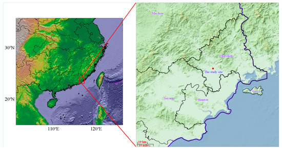
Figure 1.
Map of the study site in Chaozhou, Southeast China.
The MDA8 O3 values in Chaozhou were obtained from Qingyue Data (data.epmap.org) on 1 February 2024, the source of which is the real-time air quality release system of the Environmental Monitoring Station of the Ministry of Environmental Protection. The data from the Environmental Monitoring Station undergo rigorous quality control and quality assurance (QC/QA) processes to ensure accuracy and reliability. The O3 values are detected using ultraviolet photometric ozone analyzers, which operate based on the Beer–Lambert law. The data cover a period of 3652 days from 1 January 2014 to 31 December 2023.
2.2. KZ Filtering and Variance Analysis
The scale separation of time series of atmospheric constituent concentrations allows us to understand in more detail the patterns and substance of the changes. Rao et al. [8] and Zurbenko et al. [18] proposed the KZ filtering method as a common scale separation method, filtering KZm,p (X), where X is the original time series, and m and p are the filtering parameters, denoting the sliding window length and the number of iterations, respectively. Then, KZ15,5 (X) is the baseline component with a sliding window length of 15 days and 5 iterations, and can de-filter the short-term fluctuation factors, and KZ365,3 (X) is the long-term component with a sliding window length of 365 days and 3 iterations, and can filter out the long-term fluctuation factors. The original time series with MDA8 O3 as X can be decomposed as
where E(t) is the long-term component of MDA8 O3, which is the result of the impacts of total precursor emissions, climate, and economic changes; S(t) is the seasonal component, which is attributable to meteorological conditions such as seasonal changes in temperature (Figure S1); and W(t) is the short-term component, which is mainly affected by short-term fluctuations in precursor emissions and weather [9,19,20].
X(t) = E(t) + S(t) + W(t)
The long-term, seasonal, and short-term components are calculated, respectively, as follows:
E(t) = KZ365,3 (X)
S(t) = KZ15,5 (X) − KZ365,3 (X)
W(t) = X(t) − KZ15,5 (X)
Ideally, the MDA8 O3 original time series decomposed by the KZ filtering technique results in the short-term component, the seasonal component, and the long-term component, which are independent of each other. The variance contribution can be calculated as Equation (5), the sum of the variances of the three variables should be equal to the original time series variance, and the total covariance between them should be zero [20].
where σ2(X), σ2(W), σ2(S), and σ2(E) are the total variance, short-term component variance, seasonal component variance, and long-term component variance of the original time series of MDA8 O3, respectively; cov(E, S), cov(E, W), and cov(S, W) represent the covariance of the long-term and seasonal components, the covariance of the long-term and short-term components, and the covariance of the seasonal and short-term components, respectively. The total covariance contribution, K, can be calculated as follows:
σ2(X) = σ2(W) + σ2(S) + σ2(E) + 2 cov(E, S) + 2 cov(E, W) + 2 cov(S, W)
K = (2 cov(E, S) + 2 cov(E, W) + 2 cov(S, W))/σ2(X) = 1 − (σ2(W) + σ2(S) + σ2(E))/σ2(X)
However, the sum of the three components of the variance contribution will not be equal to 100% due to the influence of unknown factors. The closer the sum of the three components of the variance contribution is to 100% (that is, the total covariance contribution, K (Equation (6)) is approximately close to 0%), the better is the decomposition effect of the KZ filter. In addition, a relatively high percentage of variance contribution of a component means that the component is more influential on the fluctuation of the original time series. Analysis of variance (ANOVA) was performed using SPSS 23.0 software to examine the contribution of the components at different time scales to the total variance of MDA8 O3.
2.3. Percentile Regression
The classical least squares regression only reflects the degree of average variation in the MDA8 O3 concentration over time, but not the temporal variation at different percentile levels of the conditional distribution of MDA8 O3 concentrations. Koenker and Bassett [16] proposed percentile regression, which extends the least squares method from estimating conditional mean models to estimating combinations of conditional percentile functions. This approach has been applied to the long-term trend analysis of pollutants such as atmospheric particulate matter and O3 [21,22], or the analysis of factors influencing atmospheric pollutants [23]. The percentile regression method was used to analyze the temporal variation pattern of MDA8 O3 at different percentile levels.
2.4. Backward Trajectory Model and Trajectory Cluster Analysis
Combined with the reanalysis meteorological databases from the National Environmental Forecasting Center (accessed on 1 March 2024), the HYSPLIT model (HYSPLIT, https://www.ready.noaa.gov/HYSPLIT.php, National Oceanic and Atmospheric Administration) was applied to calculate the 72 h backward air mass trajectory reaching Chaozhou from 1 January 2020 to 31 December 2023. The model calculation times were 0:00, 06:00, 12:00, and 18:00 world standard time every day (the corresponding local times were 08:00, 14:00, 20:00, and 02:00 on the next day, respectively). Then, the geographic information system-based TrajStat software (version 1.5.3) was used for statistical analysis based on backward trajectories [24], including trajectory cluster analysis, trajectory sector analysis (TSA), and potential source contribution function (PSCF).
According to the spatial similarity (transmission speed and direction) of backward trajectories, trajectory cluster analysis was conducted, and obtained the trajectory clusters composed of different trajectories. On this basis, the occurrence frequency of each trajectory cluster and its corresponding O3 concentration were statistically analyzed. It was of great importance to analyze the dominant air mass direction and the potential source directions of pollutants at the study site (23.668° N, 116.633° E). In this study, TrajStat software was used to perform trajectory cluster analysis on the backward trajectories of Chaozhou City during the study period. The distance between backward trajectories was calculated by Euclidean, and the formula is as follows:
where d12 is the Euclidean distance between backward trajectories 1 and 2 (°); X1(i) and Y1(i), and X2(i) and Y2(i) represent the longitude and latitude coordinates of the spatial positioning of backward trajectories 1 and 2, respectively, at the i time interval (°); and n is the integer 72, which indicates the total running time of the backward trajectory (72 h).
2.5. TSA Analysis and PSCF Analysis
TSA analysis is a statistical method used to calculate the average pollutant concentrations corresponding to the backward trajectories in all directions of the study site, as well as to evaluate the influence of air masses from different directions on the pollutant concentration at the study site. Taking the study site (23.668° N, 116.633° E) as the center, the coverage of the backward trajectory was divided into twelve sectors with a span of 30°, which were sector 1 from due north to northeast 30° numbered clockwise to sector 12 (Figure S2). Considering that the sector may not be well defined near the origin and a small amount of curvature in the trajectory may lead to spurious results, the trajectory during the first 6 h (Figure S2) was excluded in TSA [25]. The average O3 concentration corresponding to each sector and its relative contribution to the O3 concentration in Chaozhou City are calculated as follows:
where Cj is the weighted average value of O3 mass concentrations corresponding to all backward trajectories in sector j (μg/m3); Nj is the total number of the backward trajectories; Ci is the O3 mass concentration corresponding to the i backward trajectory (μg/m3); fij and Nj are the residence times of the i backward trajectory and all backward trajectories within sector j (h), respectively; %Cj is the relative contribution of sector j to the O3 concentration in Chaozhou (%).
PSCF analysis is a statistical method that uses backward trajectories to calculate and describe the potential source contribution locations of pollutants at the study site [26]. The high value of PSCF indicates that the possibility of high concentrations of pollutants when reaching the study site after passing through the area is high, that is, the potential source of pollution. A PSCF grid layer with a cell size of 0.5° × 0.5° was created, and the PSCF values for each grid cell were calculated using the following formula:
where Pij is the PSCF value of the ij grid; mij is the residence time of the trajectory, with the O3 concentration higher than the threshold (100 μg/m3) in the ij grid when arriving at the study site through the ij grid; and nij is the residence time of all trajectories passing through the ij grid (h). To eliminate the uncertainty in potential source region judgment caused by the short residence times of grid backward trajectories and high PSCF values, Pij multiplied by the weighting factor Wij is usually used to represent the final PSCF value [27,28]. The Wij settings in this study are as follows:
3. Results and Discussion
3.1. General Characteristics of Yearly and Seasonal O3 Distribution
The annual statistics of MDA8 O3 mass concentrations in Chaozhou are given in Figure 2a. During the study period, the annual maximum value of MDA8 O3 showed a general decreasing trend (Figure S3), while the 25th and 75th percentile concentrations of MDA8 O3 ranged between 66 and 148 μg/m3, showing no clear trend. From 2006 to 2019, the average O3 concentration in the Pearl River Delta (PRD) of Guangdong Province increased significantly, and, after 2016, the growth rate of the MDA8 O3 concentration accelerated, with a value of 2.08 μg/m3 per year [29]. In order to accelerate and effectively control O3 pollution and improve air quality, Chaozhou has developed a series of measures to control the emission of air pollutants. The results show that the above control measures in Chaozhou were effective, with the MDA8 O3 concentration not showing an increasing trend as it did in the PRD of Guangdong Province, and the percentage of the MDA8 O3 concentration exceeding the secondary standard of “Ambient Air Quality Standards” (GB3095-2012) (160 μg/m3) reached the lowest value of 2.0% in 2020 (Figure 2a). This standard is an essential benchmark in assessing and managing ozone pollution levels in urban areas. Studies have shown that, during the COVID-19 pandemic, concentrations of some air pollutants in China decreased. However, in some urban areas, ozone levels increased due to reduced titration of ozone by nitrogen oxides (NOx) [30,31]. Therefore, the annual decrease in ozone concentrations in Chaozhou is not a result of the COVID-19 pandemic but rather the outcome of effective pollution control measures implemented in the region.
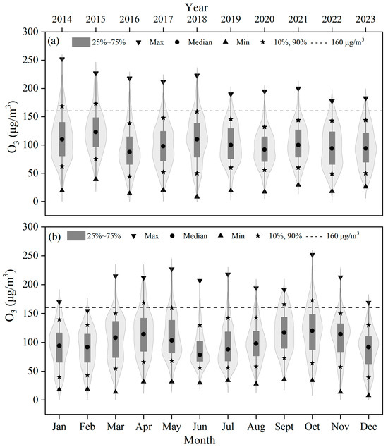
Figure 2.
Annual (a) and monthly (b) statistics of MDA8 O3 mass concentrations in Chaozhou, from 2014 to 2023.
The monthly variations in MDA8 O3 mass concentrations in Chaozhou, from 1 January 2014 to 31 December 2023 are shown in Figure 2b. Episodes of O3 pollution with higher MDA8 O3 mass concentrations (>160 μg/m3) were observed in each month, particularly in October, September, and April, with exceedance rates of 17.2%, 14.1%, and 13.1%, respectively. Generally, the middle percentiles (25th, 50th, and 75th) represent the typical cases of MDA8 O3 concentrations [32]. As shown in Figure 2b, the MDA8 O3 concentrations of the 25th, 50th, and 75th percentiles exhibited fluctuations, with double peaks occurring in October (autumn) and April (spring). Importantly, in all months, the 75th percentile values did not exceed the secondary standard (160 μg/m3). The 90th percentile of MDA8 O3 also exhibited monthly variation characteristics, forming a significant “M” shaped curve (Figure 2b). The monthly variation characteristics of MDA8 O3 were consistent with those observed in Shantou [33], a city adjacent to Chaozhou, as well as in other cities in southern China [34]. This “M” shaped curve can be explained by fluctuations in meteorological conditions and seasonal shifts in precursor emissions [34]. The lower O3 concentrations in summer may be due to the climatic characteristic of the southwest monsoon that prevails in summer, as the predominant air mass comes from the southwest cluster E (Figure S4), corresponding to lower O3 concentrations (Figure S5).
3.2. Time Series Decomposition and Analysis of MDA8 O3
The results of the time series decomposition of MDA8 O3 in Chaozhou City from 1 January 2014 to 31 December 2023, using the KZ filtering technique, are shown in Figure 3. The short-term component of the MDA8 O3 concentration in Chaozhou City exhibits frequent oscillatory fluctuations, with the main fluctuation range concentrated in −50 to 50 μg/m3. A quantile–quantile (Q-Q) plot of W(t), presented in Figure S6, indicates that W(t) essentially follows a normal distribution, suggesting that the KZ15,5 (X) filter effectively removed W(t) from X(t). The peak of the seasonal component of MDA8 O3 concentrations is less obvious, and the high value basically occurs in spring or autumn, similar to the monthly statistics in Figure 2b. The long-term components of MDA8 O3 showed an overall decreasing trend, with less fluctuation after 2018 (Figure 3d). A least squares linear regression analysis using the number of days calculated from 1 January 2014 to 31 December 2023 as the independent variable (x), and the MDA8 O3 long-term component as the dependent variable (y), yielded y = −0.00506x + 111.728 (R2 = 0.522, p < 0.0001). This predicts an annual average (365 days) decrease of 1.8 μg/m3 in the MDA8 O3 concentration in Chaozhou. This finding indicates that Chaozhou’s O3 concentration has shown a long-term downward trend over the past decade, reflecting the effectiveness of local air quality management and pollution control policies.
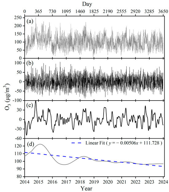
Figure 3.
The original MDA8 O3 time series (a), and its decomposition using KZ-filtering into short-term component of W(t) (b), seasonal component of S(t) (c), and long-term component of E(t) (d) in Chaozhou City.
After decomposition using the KZ filtering technique, variance analysis was also performed to examine the contribution of each time scale component to the total variance of the MDA8 O3 time series. The total covariance contribution was 12.3%, indicating that the MDA8 O3 time series were relatively well separated by KZ filtering. The contribution rates of the short-term component, seasonal component, and long-term component were 62.2%, 21.6%, and 3.8%, respectively. This indicates that the MDA8 O3 concentration is mainly affected by the short-term component, contributing 62.2%. In contrast, the long-term component also plays a role in shaping the general trend of ozone concentration, although it has a relatively small contribution.
3.3. Percentile Regression Analysis of Temporal Changes in MDA8 O3
The least squares linear regression only reflects the average change in MDA8 O3 concentrations over time, but not the temporal variation at different percentile levels of MDA8 O3. In general, the lower percentiles (5th) of MDA8 O3 represent the baseline or background concentration, the middle percentiles (25th, 50th, and 75th) represent the MDA8 O3 concentration under typical conditions, and the higher percentiles of 95th represent concentrations during O3 contamination events [32]. The health risk of O3 contamination to the exposed population should focus more on the upper percentile O3 concentrations and their trends. Therefore, using the MDA8 O3 original time series as the dependent variable (y) and the number of days starting from 1 January 2014 as the independent variable (x), regressions for the 5th, 50th, and 95th were performed to analyze the temporal changes of MDA8 O3 at different percentile levels in Chaozhou. As shown in Figure 4, the 95th percentile of the original data of MDA8 O3 exhibited a significant decreasing trend, with a predicted decrease rate of 3.2 μg/m3 per year. Meanwhile, the 50th percentile showed a slight decreasing trend, with a decrease rate of 1.6 μg/m3 per year. For the seasonal cycle of MDA8 O3, regression results for the 50th and 95th percentiles also indicate a yearly decreasing trend in O3 concentration (Figure 4). To better understand the temporal changes in different percentile levels of MDA8 O3, percentiles from 0th to 100th were divided into 99 percentiles at 1% increments. The coefficients of the independent variable, x, and the constant, C, of the percentile regression analysis are shown in Figure S7. As the percentile level of MDA8 O3 increased, the coefficient of the independent variable, x, of the percentile regression began to decrease from positive values to negative, and deviated further away from zero. It can be seen that almost all percentile regressions indicate a downward trend in ozone concentration in Chaozhou, with the degree of decrease (the coefficient of the independent variable (x)) increasing as the percentile increases.
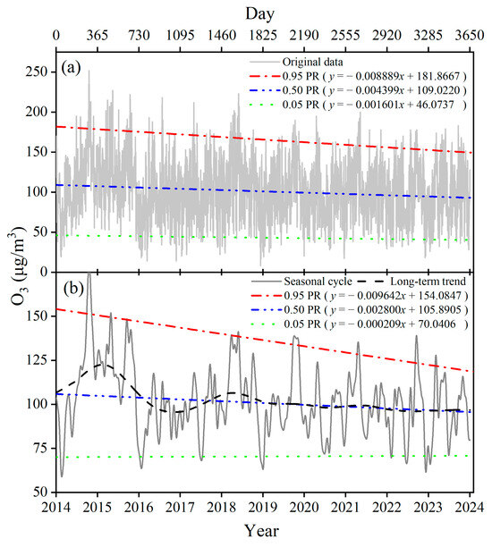
Figure 4.
Percentile regression of the original MDA8 O3 data (a) and the seasonal cycle obtained after decomposition using KZ filtering (b).
3.4. Trajectory Clusters and Transport Pathways
In this study, a total of 5844 backward trajectories from 1 January 2020 to 31 December 2023 were clustered and analyzed, and five trajectory clusters were obtained (Figure 5, detail in Figure S4). Based on the transmission distance classification, cluster A represents relatively short-distance trajectories, indicative of slow-moving backward air masses. clusters C, D, and E correspond to medium-distance trajectories. In contrast, cluster B is characterized by long-distance trajectories, rapidly transporting air masses across Inner Mongolia, Hebei, Shandong, Jiangsu, Zhejiang, and Fujian before reaching the study site in Guangdong Province. The source directions of these trajectory clusters vary, with clusters B and C originating from the northeast, cluster D from the east, cluster E from the southwest, and cluster A having no specific directional classification (Figure S4).
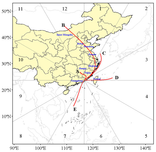
Figure 5.
The spatial distribution of the five trajectory clusters (A-E) across different sectors (1–12), where A-E represent different air mass pathways and 1–12 represent different directional segments around the study area.
Figure 6 shows the frequency and probability of occurrence of each trajectory cluster during the study period. According to this result, the trajectory clusters from different source directions ranked as follows: trajectory clusters B and C in the northeast (a total of 39.1%), trajectory cluster D in the east (27.4%) and trajectory cluster E in the southwest (24.6%). As to the seasonal differences, it was found that the northeastern trajectories (clusters B and C) dominated in winter and autumn, while the southwestern trajectory (cluster E) dominated in summer. This was basically consistent with the climate characteristics of Chaozhou, which is located in a coastal city in the subtropical monsoon region, with southerly and northerly winds prevailing in summer and winter, respectively.
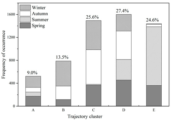
Figure 6.
Frequency and probability of occurrence for the five clusters.
Based on the comprehensive analysis of trajectory length, direction (Figure 5), frequency, probability of occurrence (Figure 6) and the corresponding O3 concentration of the trajectory cluster (Figure 7), the transport pathways of O3 pollution in Chaozhou City are described as follows. During the study period, trajectory cluster C, originating from the northeast direction, passed through Zhejiang and Fujian provinces. It had a higher probability of occurrence in autumn and winter, with the corresponding median O3 concentration being the highest at 102 μg/m3. Trajectory cluster A, without a fixed direction, belongs to a relatively short-range transport trajectory cluster with a probability of 9.0%. It originates from local areas, with a higher probability of occurrence in spring and winter, and the corresponding median O3 concentration is 100 μg/m3. Trajectory cluster E from the southwest has the highest occurrence probability in summer, with almost negligible occurrence probability in winter and autumn, with the lowest median O3 concentration of 80 μg/m3. Trajectory cluster B, originating from the northeast, passes through Inner Mongolia, Hebei, Shandong, Jiangsu, Zhejiang, and Fujian provinces, with a higher occurrence probability in autumn and winter, and the corresponding median O3 concentration is 92 μg/m3. Trajectory cluster D, originating from the east, has a corresponding median O3 concentration of 92 μg/m3.
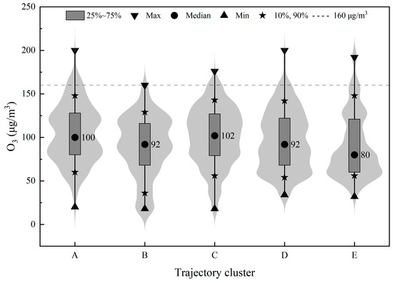
Figure 7.
Violin plots of MDA8 O3 concentrations associated with the five clusters.
3.5. Trajectory Sector Analysis of O3
The five trajectory clusters obtained by cluster analysis can reflect the specific movement pathways, distances, and source directions of various air masses in Chaozhou City (Figure 5), as well as the corresponding O3 concentrations (Figure 7). However, they do not encompass the transport of air masses in all directions and their corresponding O3 concentrations, which is crucial for gaining a comprehensive understanding of the spatial distribution and sources of O3 pollution. TSA analysis can effectively address this issue and can be mutually confirmed with the trajectory clustering results.
The backward trajectory residence time (Nj) of the 12 sectors during the study period and each season are shown in Figure 8. The top three percentages of Nj were found for sectors 2, 3, and 1, with values of 23.1%, 16.5%, and 10.7%, respectively (a total of 50.3%), indicating that the backward trajectories in the northeast were dominant. Meanwhile, the lowest three percentages of Nj were found for sectors 10, 9, and 11, with values of 1.1%, 2.4%, and 3.9%, respectively. This is consistent with the trajectory clustering results. Sectors 9, 10, and 11 have a small number of backward trajectories (Figure S4). The five trajectory clusters formed by backward trajectory clustering also do not pass through the above three sectors (Figure 5). Such results may be affected by the topography of Chaozhou, as the region is characterized by higher elevations in the north and lower elevations in the south, with mountainous terrain in the north (Figure 1). Mountain obstruction results in fewer backward trajectories in the northwest sector of the study site. The Nj in spring, autumn, and winter was similar to that during the study period. In winter, the backward trajectory in the northeast was dominant, with Nj percentages of 33.5%, 19.5%, and 18.9% for sectors 2, 3, and 1, respectively. This pattern was in line with the northerly monsoon in winter. The highest percentage of Nj in summer was in sector 7 (29.2%), followed by sector 8 (21.5%), which was consistent with the summer monsoon.
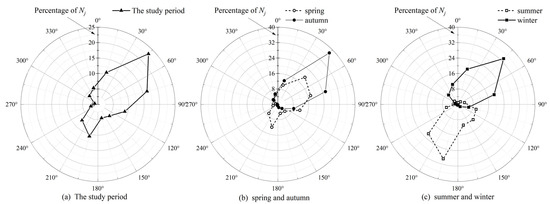
Figure 8.
Percentage of the total number of the backward trajectories (Nj) for the twelve sectors: during the study period (a), in spring and autumn (b), and in summer and winter (c).
The average concentration of O3 corresponding to each sector (Cj) is shown in Figure 9. The average concentration of O3 in sectors 3 and 2 was as high as 101.5 and 99.5 μg/m3, respectively. The sector analysis is basically consistent with the trajectory cluster results, with the northeast direction corresponding to high concentrations of O3. Meanwhile, the Nj percentages of sectors 1, 2, and 3 were 10.7%, 23.1%, and 16.5% respectively, resulting in a higher relative contribution (%Cj) of 10.6%, 24.1%, and 17.5% (a total of 52.2%). In contrast, due to the relatively low percentage of Nj, sectors 10, 9, and 11 also had lower relative contribution percentages of O3, which were 1.1%, 2.3%, and 3.8%, respectively. Thus, TSA result suggests that the northeast direction (sectors 1, 2, and 3) contributed about half (50.3%) of the backward air mass trajectory extraction time during the study period, and also contributed about half of the O3 weighted concentration in Chaozhou City (52.2%).
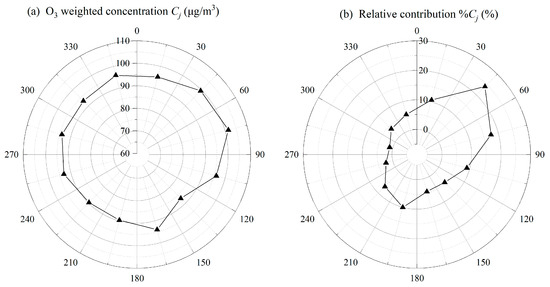
Figure 9.
Sector average concentration (a) and relative contribution (b) for O3 in Chaozhou during the study period.
3.6. PSCF Analysis of O3
The trajectory cluster analysis and TSA can identify the main transport pathways and source directions of high O3 concentrations in Chaozhou, but cannot locate the specific position contributing to O3 at the study site. To address this limitation, PSCF analysis was performed utilizing backward trajectories and O3 data from the study period. As illustrated in Figure 10, high PSCF values (>0.5) are predominantly found in sectors 2, 3, and 1 in the northeast direction, covering the major pathways of cluster C with higher O3 concentrations (Figure 7). This suggests that there may be strong pollution emission sources in these areas. Conversely, PSCF values in the southeast, southwest, and northwest directions are generally lower. Seasonal analysis reveals that PSCF values are typically reduced in summer (June–August) and winter (December–February) due to comparatively lower O3 concentrations during these periods (Figure S5), as evidenced by the limited number of days with concentrations exceeding 160 μg/m3 (Figure 2). In contrast, a higher proportion of days with O3 concentrations exceeding 160 μg/m3 occurs in spring (March–May) and particularly in autumn (July–September). The backward trajectory air masses in autumn mainly come from the northeast (Figure S8), which is basically consistent with the distribution of high PSCF values. NMVOC and NOx emission maps obtained from the China MEIC emission database [35] further confirm these findings. According to the 2020 emission map (Figure S9), the highest NMVOC emissions are observed in densely populated and developed areas, especially in the eastern and southern coastal provinces of Jiangsu, Shandong, Zhejiang (Sectors 1 and 2), and the PRD area of Guangdong (Sector 9). Similarly, the highest NOx emissions are also found in these coastal provinces. The spatial distribution of these emissions confirms that there are high ozone precursor emissions in the northeast of the study site, and the high O3 concentrations in Chaozhou may be affected by regional transport from these high-emission regions. However, during spring, both Chaozhou and its surrounding areas show high PSCF values (>0.5), suggesting that O3 pollution may result from both regional transport and local emissions. This finding aligns with the precursor emission data from the China MEIC emission database (Figure S9).
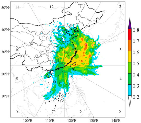
Figure 10.
Distribution map of PSCF values for MDA8 O3, where sectors 1 to 12 represent different directional segments around the study area.
4. Conclusions
This study comprehensively analyzed the temporal trends and spatial sources of surface O3 in Chaozhou. Our findings indicate a general long-term downward trend in the MDA8 O3 concentrations, despite significant monthly fluctuations. Notably, the peak concentrations of MDA8 O3 typically emerged in October (autumn) and April (spring). The analysis indicates that more than 62.2% of the variability in MDA8 O3 concentrations was driven by short-term variations in environmental factors, while long-term contributions had minimal impact. This highlights the significant influence of immediate meteorological conditions and transient pollution events on local O3 levels.
Furthermore, statistical analysis based on backward trajectories was used to provide deep insights into the transport pathways and sources of surface O3, from 1 January 2020 to 31 December 2023. Air masses from the northeast, particularly from clusters B and C, were identified as major contributors to elevated O3 levels in Chaozhou, accounting for 39.1% of the air masses during the study period. These findings were corroborated by TSA results, which showed significant contributions from the northeast sectors, underscoring the critical role of regional transport in shaping O3 pollution in Chaozhou. The PSCF analysis further supported this, pinpointing the northeast as a significant potential source region, especially during the autumn months when O3 levels peak. The PSCF result for the spring period showed that local source emissions also contributed to high O3 concentrations.
In summary, this study elucidates the temporal trends and spatial sources of O3 pollution in Chaozhou. Given the significant role of regional transport, enhanced cooperation among regional stakeholders is essential to effectively manage and mitigate O3 pollution.
Supplementary Materials
The following supporting information can be downloaded at: https://www.mdpi.com/article/10.3390/atmos15070777/s1. Figure S1: Monthly meteorological data of Chaozhou city in 2023; Figure S2: The backward trajectory during the first 6 h at study site; Figure S3: A linear regression analysis of the annual maximum values of MDA8 O3; Figure S4: Backward trajectories for different clusters at the study site from 1 January 2020 to 31 December 2023; Figure S5: Seasonal distribution map of PSCF values for MAD8 O3; Figure S6: A quantile-quantile (Q-Q) plot of W(t); Figure S7: Percentile regression coefficient of O3 ((a) coefficient of independent variable x; (b) Constant C); Figure S8: Backward trajectories at study site for each season, from 1 January 2020 to 31 December 2023; Figure S9: NWVOC (a) and NOx (b) emissions in the area surrounding the study site in 2020.
Author Contributions
Data curation, Z.H.; methodology, Z.H.; writing—original draft preparation, Z.H.; writing—review and editing, L.T.; project administration, L.T.; validation, X.Z.; visualization, J.S.; software, S.L.; formal analysis, H.X. All authors have read and agreed to the published version of the manuscript.
Funding
This research was supported by Ningbo Natural Science Foundation (No. 2023J059); Guangxi Key Research and Development Programme (No. GuikeAB21220063); Chaozhou Science and Technology Plan Project (No. 2018GY03); Chaozhou Philosophy and Social Sciences 14th Five Year Plan Project (No. 2023-C-15).
Institutional Review Board Statement
Not applicable.
Informed Consent Statement
Not applicable.
Data Availability Statement
The data presented in this study are available on reasonable request from the corresponding author.
Acknowledgments
Thanks to Qingyue Data (data.epmap.org, accessed on 1 February 2024) for support of environmental data. We also thank anonymous reviewers for their valuable comments to improve the quality of the manuscript.
Conflicts of Interest
The authors declare no conflicts of interest.
References
- Nuvolone, D.; Petri, D.; Voller, F. The effects of ozone on human health. Environ. Sci. Pollut. Res. 2017, 25, 8074–8088. [Google Scholar] [CrossRef]
- Zhang, J.; Wei, Y.; Fang, Z. Ozone pollution: A major health hazard worldwide. Front. Immunol. 2019, 10, 2518. [Google Scholar] [CrossRef] [PubMed]
- Jurán, S.; Edwards-Jonášová, M.; Cudlín, P.; Zapletal, M.; Šigut, L.; Grace, J.; Urban, O. Prediction of ozone effects on net ecosystem production of Norway spruce forest. iForest Biogeosci. For. 2018, 11, 743–750. [Google Scholar] [CrossRef]
- Singh, A.A.; Agrawal, S.B. Tropospheric ozone pollution in India: Effects on crop yield and product quality. Environ. Sci. Pollut. Res. 2017, 24, 4367–4382. [Google Scholar] [CrossRef]
- Yang, J.; Hu, Y.; Peltier, W.R. Radiative effects of ozone on the climate of a Snowball Earth. Clim. Past. 2012, 8, 2019–2029. [Google Scholar] [CrossRef]
- Department of Science and Technology Standards, Ministry of Environmental Protection. Ambient Air Quality Standards GB3095-2012; China Environmental Science Press: Beijing, China, 2012. [Google Scholar]
- Li, K.; Jacob, D.J.; Liao, H.; Shen, L.; Zhang, Q.; Bates, K.H. Anthropogenic drivers of 2013-2017 trends in summer surface ozone in China. Proc. Natl. Acad. Sci. USA 2019, 116, 422–427. [Google Scholar] [CrossRef]
- Rao, S.T.; Zurbenko, I.G. Detecting and tracking changes in ozone air quality. J. Air Waste Manag. Assoc. 1994, 44, 1089–1092. [Google Scholar] [CrossRef]
- Rao, S.T.; Zurbenko, I.G.; Neagu, R.; Porter, P.S.; Ku, J.Y.; Henry, R.F. Space and time scales in ambient ozone data. Bull. Am. Meteorol. Soc. 1997, 78, 2153–2166. [Google Scholar] [CrossRef]
- Ma, Z.; Xu, J.; Quan, W.; Zhang, Z.; Lin, W.; Xu, X. Significant increase of surface ozone at a rural site, north of eastern China. Atmos. Chem. Phys. 2016, 16, 3969–3977. [Google Scholar] [CrossRef]
- Song, X.; Hao, Y. Analysis of ozone pollution characteristics and transport paths in Xi’an City. Sustainability 2022, 14, 6146. [Google Scholar] [CrossRef]
- Wang, M.; Yim, S.H.; Wong, D.; Ho, K. Source contributions of surface ozone in China using an adjoint sensitivity analysis. Sci. Total Environ. 2019, 662, 385–392. [Google Scholar] [CrossRef] [PubMed]
- Dimitriou, K.; Kassomenos, P. Three year study of tropospheric ozone with back trajectories at a metropolitan and a medium scale urban area in Greece. Sci. Total Environ. 2015, 502, 493–501. [Google Scholar] [CrossRef] [PubMed]
- Tong, L.; Zhang, J.; Xu, H.; Xiao, H.; He, M.; Zhang, H. Contribution of regional transport to surface ozone at an island site of Eastern China. Aerosol Air Qual. Res. 2018, 18, 3009–3024. [Google Scholar] [CrossRef]
- Chen, Y.; Yan, H.; Yao, Y.; Zeng, C.; Gao, P.; Zhuang, L.; Fan, L.; Ye, D. Relationships of ozone formation sensitivity with precursors emissions, meteorology and land use types, in Guangdong-Hong Kong-Macao Greater Bay Area, China. J. Environ. Sci. 2020, 94, 1–13. [Google Scholar] [CrossRef]
- Kim, J.S.; Zhou, W.; Cheung, H.N.; Chow, C.H. Variability and risk analysis of Hong Kong air quality based on Monsoon and El Nino conditions. Adv. Atmos. Sci. 2013, 30, 280–290. [Google Scholar] [CrossRef]
- Huang, Z.; Zhang, H.; Tong, L.; Zhang, J.; Chen, J. Evaluatng the impacts of regional transport and monsoons on the air quality in Nanjing based on VAR model. Glob. Environ. Health Saf. 2018, 2, 1–11. [Google Scholar]
- Zurbenko, I.; Porter, P.S.; Rao, S.T.; Ku, J.Y.; Gui, R.; Eskridge, R.E. Detecting discontinuities in time series of upper-air data: Development and demonstration of an adaptive filter technique. J. Clim. 1996, 9, 3548–3560. [Google Scholar] [CrossRef]
- Wise, E.K.; Comrie, A.C. Extending the Kolmogorov-Zurbenko filter: Application to ozone, particulate matter, and meteorological trends. J. Air Waste Manag. Assoc. 2005, 55, 1208–1216. [Google Scholar] [CrossRef]
- Wu, Y.-H.; Bai, H.M.; Shi, H.D.; Li, X.-C.; Gao, C.X.; Song, H. Assessing the influence of weather conditions on the change of air quality in Hohhot. Arid. Zone Res. 2016, 33, 292–298. [Google Scholar]
- Barmpadimos, I.; Keller, J.; Oderbolz, D.; Hueglin, C.; Prevot, A.S.H. One decade of parallel fine (PM2.5) and coarse (PM10-PM2.5) particulate matter measurements in Europe: Trends and variability. Atmos. Chem. Phys. 2012, 12, 3189–3203. [Google Scholar] [CrossRef]
- Monteiro, A.; Carvalho, A.; Ribeiro, I.; Scotto, M.; Barbosa, S.; Alonso, A.; Baldasano, J.M.; Pay, M.T.; Miranda, A.I.; Borrego, C. Trends in ozone concentrations in the Iberian Peninsula by quantile regression and clustering. Atmos. Environ. 2012, 56, 184–193. [Google Scholar] [CrossRef]
- Xuechao, L. The influencing factors on PM2.5 concentration of lanzhou based on quantile regression. J. Hebei Geo. Univ. 2018, 41, 61–68. [Google Scholar] [CrossRef]
- Wang, Y.Q.; Zhang, X.Y.; Draxler, R.R. TrajStat: GIS-based software that uses various trajectory statistical analysis methods to identify potential sources from long-term air pollution measurement data. Environ. Model. Softw. 2009, 24, 938–939. [Google Scholar] [CrossRef]
- Bari, A.; Dutkiewicz, V.A.; Judd, C.D.; Wilson, L.R.; Luttinger, D.; Husain, L. Regional sources of particulate sulfate, SO2, PM2.5, HCl, and HNO3, in New York, NY. Atmos. Environ. 2003, 37, 2837–2844. [Google Scholar] [CrossRef]
- Cheng, M.D.; Hopke, P.K.; Barrie, L.; Rippe, A.; Olson, M.; Landsberger, S. Qualitative determination of source regions of aerosol in Canadian high Arctic. Environ. Sci. Technol. 1993, 27, 2063–2071. [Google Scholar] [CrossRef]
- Han, Y.-J.; Holsen, T.M.; Hopke, P.K.; Yi, S.-M. Comparison between back-trajectory based modeling and Lagrangian backward dispersion modeling for locating sources of reactive gaseous mercury. Environ. Sci. Technol. 2005, 39, 1715–1723. [Google Scholar] [CrossRef]
- Li, M.; Huang, X.; Zhu, L.; Li, J.; Yu, S.; Cai, X.; Xie, S. Analysis of the transport pathways and potential sources of PM10 in Shanghai based on three methods. Sci. Total Environ. 2012, 414, 525–534. [Google Scholar] [CrossRef] [PubMed]
- Zhao, W.; Gao, B.; Lu, Q.; Zhong, Z.; Liang, X.; Liu, M.; Ma, S.; Sun, J.; Chen, L.; Fan, S. Ozone pollution trend in the Pearl River Delta region during 2006–2019. Environ. Sci. 2021, 42, 97–105. [Google Scholar] [CrossRef]
- Pei, Z.; Han, G.; Ma, X.; Su, H.; Gong, W. Response of major air pollutants to COVID-19 lockdowns in China. Sci. Total Environ. 2020, 743, 140879. [Google Scholar] [CrossRef]
- He, G.; Pan, Y.; Tanaka, T. The short-term impacts of COVID-19 lockdown on urban air pollution in China. Nat. Sustain. 2020, 3, 1005–1011. [Google Scholar] [CrossRef]
- Li, J.; Lu, K.; Lv, W.; Li, J.; Zhong, L.; Ou, Y.; Chen, D.; Huang, X.; Zhang, Y. Fast increasing of surface ozone concentrations in Pearl River Delta characterized by a regional air quality monitoring network during 2006–2011. J. Environ. Sci. 2014, 26, 23–36. [Google Scholar] [CrossRef] [PubMed]
- LI, J.; LI, C.; XIAO, L.; GUO, Y.; HUANG, Y.; CHEN, S.; CHEN, M.; LI, W.; ZHANG, Y. Characteristics and meteorological conditions of ozone pollution in Shantou city. Meteorol. Environ. Res. 2021, 12, 19–25. [Google Scholar] [CrossRef]
- Yang, G.; Liu, Y.; Li, X. Spatiotemporal distribution of ground-level ozone in China at a city level. Sci. Rep. 2020, 10, 7229. [Google Scholar] [CrossRef] [PubMed]
- Li, M.; Liu, H.; Geng, G.; Hong, C.; Liu, F.; Song, Y.; Tong, D.; Zheng, B.; Cui, H.; Man, H.; et al. Anthropogenic emission inventories in China: A review. Natl. Sci. Rev. 2017, 4, 834–866. [Google Scholar] [CrossRef]


Disclaimer/Publisher’s Note: The statements, opinions and data contained in all publications are solely those of the individual author(s) and contributor(s) and not of MDPI and/or the editor(s). MDPI and/or the editor(s) disclaim responsibility for any injury to people or property resulting from any ideas, methods, instructions or products referred to in the content. |
© 2024 by the authors. Licensee MDPI, Basel, Switzerland. This article is an open access article distributed under the terms and conditions of the Creative Commons Attribution (CC BY) license (https://creativecommons.org/licenses/by/4.0/).