Abstract
This study evaluates nine Planetary Boundary Layer (PBL) turbulence parameterization schemes from the Weather Research and Forecasting (WRF) mesoscale meteorological model, comparing hourly values of meteorological variables observed and simulated at the surface of the Metropolitan Region of São Paulo (MRSP). The numerical results were objectively compared with high-quality observations carried out on three micrometeorological platforms representing typical urban, suburban, and rural land use areas of the MRSP, during the 2013 summer and winter field campaigns as part of the MCITY BRAZIL project. The main objective is to identify which PBL scheme best represents the diurnal evolution of conventional meteorological variables (temperature, relative and specific humidity, wind speed, and direction) and unconventional (sensible and latent heat fluxes, net radiation, and incoming downward solar radiation) on the surface. During the summer field campaign and over the suburban area of the MRSP, most PBL scheme simulations exhibited a cold and dry bias and overestimated wind speed. They also overestimated sensible heat flux, with high agreement index and correlation values. In general, the PBL scheme simulations performed well for latent heat flux, displaying low mean bias error and root square mean error values. Both incoming downward solar radiation and net radiation were also accurately simulated by most of them. The comparison of the nine PBL schemes indicated the local Mellor-Yamada-Janjic (MYJ) scheme performed best during the summer period, particularly for conventional meteorological variables for the land use suburban in the MRSP. During the winter field campaign, simulation outcomes varied significantly based on the site’s land use and the meteorological variable analyzed. The MYJ, Bougeault-Lacarrère (BouLac), and Mellor-Yamada Nakanishi-Niino (MYNN) schemes effectively simulated temperature and humidity, especially in the urban land use area. The MYNN scheme also simulated net radiation accurately. There was a tendency to overestimate sensible and latent heat fluxes, except for the rural land use area where they were consistently underestimated. However, the rural area exhibited superior correlations compared to the urban area. Overall, the MYJ scheme was deemed the most suitable for representing the convectional and nonconventional meteorological variables on the surface in all urban, suburban, and rural land use areas of the MRSP.
1. Introduction
The Planetary Boundary Layer (PBL) is characterized by the presence of turbulence, an essential mechanism for the diffusion of atmospheric properties [1,2]. Accurate representation of turbulence is extremely important for improving numerical weather and climate predictions, especially for severe weather events such as storms, tornadoes, and hurricanes in the context of climate change [3,4,5]. In addition, understanding turbulent movements is vital for assessing the dispersion potential of atmospheric pollutants, which has direct implications for air quality [6,7,8,9].
Despite significant advances in numerical weather prediction, mesoscale models still face challenges related to adequately representing turbulence in the PBL under continued demand to improve spatial and temporal resolutions. To overcome this limitation, mesoscale models rely on several PBL turbulence parameterization schemes [1,2,10]. In the case of the Weather Research and Forecasting (WRF) model, the performance of PBL parameterization schemes has been systematically analyzed for improving air quality assessments and predicting severe weather events [8,9,11,12,13], and in simulating flows over regions with complex topography and heterogeneous land cover [7,14,15,16,17,18]. Most of these studies are based on simulations of atmospheric properties in continental regions located at mid-latitudes, mainly in North America [5,18,19,20,21], Europe [7,8,9,14,22,23,24,25], and Asia [12,16,26,27,28,29]. In general, these studies have shown that the performance of the WRF model depends on horizontal and temporal resolution, number of vertical levels, initial conditions, PBL turbulence parameterization scheme, simulated atmospheric conditions, and geographical features of the region of interest [8,9,13].
Due to the complexity and variability of these factors, different model configurations can generate substantially different results. Therefore, the choice of parameters and model configuration must comply with the criteria linked to the study scenario in question. This context highlights the need for a detailed evaluation, considering the multiple PBL turbulence parameterization schemes available in WRF, to choose the one that best represents the characteristics of the study region.
In this sense, this study focuses on simulating the diurnal evolution of PBL properties at the surface in the Metropolitan Region of São Paulo (MRSP, Figure 1) with the WRF model using nine PBL turbulence parameterization schemes. The scientific literature presents a variety of PBL scheme analyses, indicating its advantages and limitations [5,13,21]. However, a straightforward application of these analyses cannot be carried out for a complex region such as MRSP without previous verification. The choice of this region is strategic due to its unique climate, land use, and topography, representing a real challenge for mesoscale modeling. The main purpose is to determine which PBL scheme is most appropriate for the MRSP.
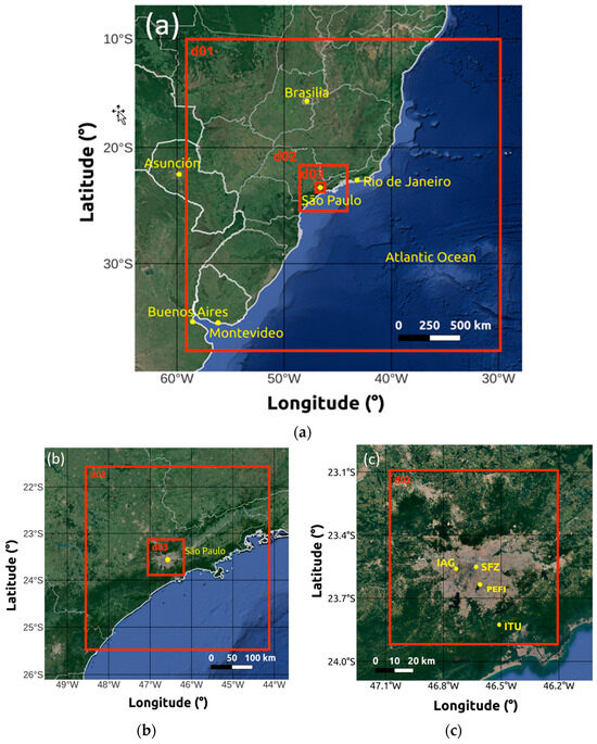
Figure 1.
Geographic features of the MRSP (indicated by São Paulo) considering the configurations of tree domains used in the WRF model simulations. (a) Indicates the parent domain d01, with 3000 km × 3000 km and grid resolution of 15 km. (b) Indicates the first nested grid d02, with 453 km × 453 km and grid resolution of 3 km. (c) Indicates the innermost higher resolution grid d03, with 90.6 km × 90.6 km and grid resolution of 0.6 km. The innermost grid domain d03 covers the urbanized area of the MRSP and the three micrometeorological platforms IAG (suburban), SFZ (urban), and ITU (rural).
Therefore, the analysis performed here will be based on hourly values of conventional (temperature, relative and specific humidity, wind speed, and direction) and unconventional (sensible and latent heat fluxes, net radiation, and incoming downward solar radiation) meteorological variables observed on the surface of the MRSP, over 10 consecutive days in the summer (19–28 February) and 10 consecutive days in the winter (6–15 August) of 2013, as part of the MCITY (MegaCITY) BRAZIL project [30]. These high-quality observational datasets were measured at three sites located in areas characterized by urban, suburban, and rural land use and indicated by SFZ (“Secretaria da FaZenda” building), IAG (Institute of Astronomy, Geophysics, and Atmospheric Science building) and ITU (“ITUtinga Pilões” State Park) in Figure 1c, respectively. The choice of these variables aims to provide a comprehensive understanding of surface–atmosphere interaction over subtropical megacities such as São Paulo, considering not only conventional meteorological variables but also unconventional ones that indicate energy and radiation exchanges at the surface. These observations will be objectively compared with WRF model simulations using the following nine PBL turbulence parameterization schemes: Mellor-Yamada Janjic (MYJ), Mellor-Yamada Nakanishi-Niino (MYNN), Quasi-Normal Scale Elimination (QNSE), University of Washington (UW), Bougeault-Lacarrère (BouLac), Yonsei University (YSU), Shin-Hong (SH), Asymmetric Convective Model (ACM2), and Total Energy-Mass flux (TEMF).
Despite the shortness of the dataset, the combination of conventional and nonconventional meteorological variables confers originality to this study. As such, it will not only contribute to the optimization of atmospheric modeling in this specific region but can also be used as a guide for future WRF modeling studies in tropical and subtropical urban areas, where a more accurate representation of the PBL is essential for improving understanding of local meteorological phenomena on the urban climate.
This article is organized as follows: Section 2 describes the climate, the meteorological conditions, and the observations during the summer and winter field campaigns in the MRSP. The main features of the WRF model configuration, the nine PBL turbulence parameterization schemes, and the statistical parameters used to objectively assess their performance are also described in Section 2. The results of the model performance evaluation are presented in Section 3. Finally, the summary and conclusions are presented in Section 4.
2. Materials and Methods
2.1. Region of Study
The São Paulo Megacity and 38 neighboring cities shape the MRSP (Figure 1). This region, located approximately 60 km from the Atlantic Ocean, has around 21.73 million inhabitants [31]. Its area comprises 7947 km2, making it the largest urban area in South America and one of the ten largest in the world. The São Paulo Megacity occupies the central portion of the MRSP, has a population of 11.45 million inhabitants, and its center (23°30′ S, 46°40′ W) is located 760 m above mean sea level.
According to the Köppen-Geiger classification [32], the climate in MRSP can be characterized as high-elevation subtropical humid (Cwb). The climate is typical of subtropical regions, alternating a dry and moderately cold winter (June–August) with a humid and hot summer (December–February). On average, the annual accumulated rain in the MRSP reaches 1500 mm, while the monthly accumulated precipitation values are higher during the summer, with a maximum of 232.14 mm in January, and lower during the winter, with a minimum of 38.01 mm in August. The seasonal variation in temperature in the MRSP is modulated by altitude (~700 m) and maritime effects, with the monthly average temperature reaching a maximum of 21.9 °C in February and a minimum of 15.3 °C in July. The seasonal variation in surface winds in the MRSP is controlled by the position and relative intensity of the South Atlantic Subtropical High and the Continental Low [33]. These two systems combined induce N–NE winds during the summer and NE–E winds during the winter, and monthly average wind speed values varying from a minimum of 1.7 ms−1 in May to a maximum of 2.3 m s−1 in December.
The weather and climate patterns of the MRSP are frequently affected by synoptic and mesoscale disturbances, mainly by the passage of Cold Front (CF) and Sea Breeze (SB). In general, CFs induce pre-frontal NW winds and post-frontal SE winds in the MRSP. Despite the distance from the Atlantic Ocean (~60 km), SB penetrates the MRSP on more than 50% of the days of the year, accompanied by changes in wind direction from NW to SE and by a sharp drop in temperature and rise in relative humidity [30,33,34].
On average, the PBL height reaches a maximum of 1632 ± 96 m in May and a minimum of 1061 ± 77 m in September. This behavior is attributed to the seasonal variation in the cloud pattern due to the influence of synoptic and mesoscale systems [33]. In general, the Urban Heat Island (UHI) intensity in the MRSP displays a minimum during the day and two maxima, a primary during the day and a secondary maximum at night. The daytime minimum UHI intensity varies from 0.5 to 2 °C and occurs between 09:00 and 13:00 LT. The primary daytime maxima UHI intensities vary from 3.5 to 5 °C and occur between 14:00 and 17:00 LT in January and August, respectively. During these months, a secondary maximum of ~4.6 °C occurs at night [30]. During the day, the UHI intensity tends to decrease or be less pronounced compared to the night due to the cooling effects of SB in the MRSP.
The climate in the MRSP is also influenced by the Low-Level Jet (LLJ). They occur on 77.6% of days, with a maximum in December (85.5% of days) and a minimum in June (70% of days). The intensity and height of the LLJ show little seasonal variation, with an average intensity of 7.8 ± 0.1 m s−1, height of 640 ± 151 m, and direction mainly E and SE. During the MCITY BRAZIL Project’s 2013 field campaigns, 76.4% of the LLJ events were generated by the inertial oscillation mechanism and 35.3% of them were combined with the passage of the SB. The LLJ intensity was negatively correlated with the intensity of the Surface Inversion Layer (SIL) strength and UHI intensity, particulate matter 2.5, and carbon monoxide concentrations, indicating that turbulent mixing and horizontal advection produced by the LLJ contribute to reducing them in the MRSP [35].
2.2. Observation
To evaluate the performance of the WRF model, the numerical results were compared with high-quality observations carried out in the MRSP over 20 days in 2013. They correspond to two field campaigns of the MCITY BRAZIL Project carried out over 10 consecutive days in the summer (19–28 February) and 10 consecutive days in the winter (6–15 August). These observations comprise hourly values of conventional and unconventional meteorological variables measured at the surface. Conventional meteorological variables are temperature (T), relative humidity (RH), specific humidity (q), wind speed (WSP), and wind direction (WDIR). Non-conventional meteorological variables are the main components of the energy and radiation balance at the surface such as net radiation (RN), vertical turbulent fluxes of sensible (H), latent (LE) heat, and incoming downward solar radiation (DSR). The observed values of q were estimated from simultaneously observed values of T and RH. They were included in this analysis because q is a better indicator of water vapor load in the atmosphere.
Surface variables were measured simultaneously on the three micrometeorological platforms of the MCITY BRASIL Project: IAG, SFZ, and ITU. The site IAG is on the campus of the University of São Paulo, west of the city of São Paulo, in an area representative of suburban land use (Figure 1c). The site SFZ is in the center of São Paulo City, in an area representative of urban land use. The site ITU is in the extreme south of the MRSP, between the municipalities of São Bernardo do Campo and Cubatão, in an area representative of rural land use occupied by Atlantic Forest reforestation. The IAG site was operational during both summer and winter field campaigns in February (19–28) and August (6–15) of 2013. Due to operational problems, both SFZ and ITU sites were operational only during the winter field campaign in August (6–15) of 2013.
2.2.1. Sensor’s Description
Horizontal wind speed and direction were measured using an anemometer, model 034B, manufactured by MetOne Instruments Inc, Oregon, USA, installed 25.4 m (IAG), 85.0 m (SFZ), and 9.7 m (ITU) from the surface. Temperature and relative humidity measurements were taken using temperature and relative humidity sensors, model CS215, manufactured by Campbell Sci Inc, Logan, UT, USA, installed 18.7 m (IAG), 78.6 m (SFZ), and 1.6 m (ITU) from the surface. Observations of net radiation and its four components (including incoming downward solar radiation) were made using a net radiometer, model CNR4, manufactured by Kipp-Zonen, Netherlands, installed 24 m (IAG), 9.4 m (ITU), and 83.8 m (SFZ) from the surface.
All these variables were measured continuously with a sampling frequency of 0.05 Hz and stored as a 5 min average. The 5 min time series values for all variables were subject to a quality control procedure that removes spurious values caused by sensor malfunctions, inadequate sensor exposure, accumulation of dust, soot, and water from rain and dew, communication problems between the sensor and acquisition system, and transmission of data caused by internet problems. A complete description of the quality control procedures applied to measurements used in this work is described in Oliveira et al. [30]. A more detailed description of the sensors deployed to measure the variables in this work can be found in Oliveira et al. [30], Sánchez et al. [33], and Silveira et al. [36]. Table 1 summarizes these three sites and sensor features.

Table 1.
Summary of the observational sites and sensor features.
2.2.2. Vertical Turbulent Fluxes of Sensible and Latent Heat
The vertical turbulent fluxes of sensible and latent heat were estimated using the MBFLUX (Mcity-Brazil FLUX) algorithm (Oliveira et al. [30]; Silveira et al. [36]). In this algorithm, the eddy covariance method is used to estimate H and LE from 30 min blocks of vertical velocity, air temperature, and water vapor density values observed simultaneously at a frequency of 10 Hz. These measurements are carried out using a three-dimensional sonic anemometer coupled to a gas analyzer, model IRGASON, manufactured by Campbell Scientific Inc., Logan, UT, USA, and installed at 25.4 m (IAG), 85.0 m (SFZ) and 9.4 m (ITU). The quality control procedure consisted of Webb correction, linear trend removal, enforcement of asymmetry and skewness thresholds, non-stationarity detection tests and removal, removing the effects of tower blocking, rain, and dew accumulations on the sensors, and correction of anemometer misalignment in the vertical direction using the Planar Fit method [30,36]. The quality control procedure removed 40.5% of the 962 valid blocks at IAG, and 61% and 33.5% of the 481 blocks at ITU and SFZ, respectively. It should be emphasized that hourly values of all variables used in this work correspond to measurements carried out over 20 days in the IAG (10 days in the summer and 10 days in the winter field campaigns); 10 days in ITU and SFZ (10 days in the winter field campaign of 2013). Unfortunately, the micrometeorological platforms of ITU and SFZ were not operational in the summer field campaign.
2.3. Meteorological Conditions during the Field Campaigns
The meteorological conditions observed in the MRSP during the summer field campaign of 2013 (19–28 February) were determined by the influence of the Bolivia High (BH), the Upper Tropospheric Cyclonic Vortex (UTCV), and the western border of the Sout-Atlantic Subtropical High (SASH). For five days (19–21, 24, and 25 February), clear skies predominated, associated with the subsidence induced by the UTCV positioned to the northeast of MRSP. The conditions of instability and precipitation were associated with the presence of a shortwave Upper Air Trough at medium levels (22–23 February) and the combination of the border of the SASH at low levels and the difluence of the flow at 250 hPa induced by the combination of the BH and the UTCV (26–28 February). These conditions induced horizontal mass divergence at high levels and convergence in the lower layers of the troposphere, favoring the formation of large vertical clouds.
Likewise, conditions of strong daytime heating and the passage of SB also contributed to the occurrence of precipitation, for example, during the afternoon of 24 February, 14.7 mm of precipitation was recorded at the PEFI climate surface station (Figure 1c) associated with these conditions [33]. In general, in the MRSP, the penetration of SB occurs in the early afternoon and is characterized by a sharp drop in air temperature and an increase in wind speed, cloudiness, and relative humidity, as well as a change in wind direction from NE to SE [34,37]. Five SB events were observed during this period (19–20, 24, 27, and 28 February) [33,37]. In these cases, the convective growth of the PBL was interrupted, reducing PBL height compared to clear sky days [33].
On the other hand, during the 10-day field campaign in the winter of 2013 (6–15 August), the atmospheric conditions were under the influence of the anticyclonic circulation associated with SASH. This pattern dominated the flow throughout the tropospheric column, inhibiting the formation of clouds and precipitation. However, on the 11th and 14th, these conditions were altered by the passage of frontal systems. On these two days, the presence of abundant cloudiness and the occurrence of precipitation limited thermal convection, and the development of PBL was due to the mechanical production of Turbulent Kinetic Energy (TKE). In addition, only one case of SB was observed on 6 August.
2.4. WRF Model Configuration
For this study, version 4.1.2 of the WRF ARW model was used [38]. Three nested domains and grid resolutions are configured for the study region (Figure 1). The parent horizontal domain (d01) has a 15 km grid resolution covering an area of 3000 × 3000 km. The parent domain is centered at 23.49° S and 44.50° W and includes parts of southeastern South America and the western South Atlantic Ocean (Figure 1a). The first nested domain (d02) has a 3 km grid resolution covering an area of 453 km by 453 km. This nested domain is centered at 23.58° S and 46.34° W and represents the southeastern region of the state of São Paulo (Figure 1b). The innermost higher resolution domain (d03) has a 0.6 km grid resolution covering an area of 90.6 km by 90.6 km. This domain is centered at 23.50° S and 46.63° W and represents the most urbanized part of the MRSP (Figure 1c). The domain in the vertical direction was set with 38 levels, containing 25 levels in the first 4000 m of the atmosphere.
Initial and boundary conditions were obtained from the National Center for Environmental Prediction—Global Forecast System (NCEP-GFS) analyses. Final analysis (FNL) data are the operational global analysis data available on 1° × 1° grids in six hourly time steps. FNL is available at 27 pressure levels, ranging from the surface (1000 hPa) to 10 hPa (http://rda.ucar.edu/datasets/ds083.2/, accessed on 26 June 2024). For geographic data, such as topography and land use, standard datasets from the U.S. Geological Survey (USGS, http://www.usgs.gov/, accessed on 26 June 2024) with 30 arc-second resolutions for domains d01 and d02. For domain d03, the topography was obtained from the Shuttle Radar Topography Mission (SRTM) dataset with a resolution of 30 m (http://www2.jpl.nasa.gov/srtm, accessed on 26 June 2024) [39,40].
Table 2 shows the main physical parameterizations selected in the simulations carried out in this work. More information on these parameterizations can be found in Shamrock et al. [38].
Table 2.
Main physical process parametrizations used in the WRF model simulations.
To represent the land surface, the Noah Land Surface Model (LSM) was coupled with the Single Layer Urban Canopy Model (SLUCM), developed by Kusaka et al. [46] and Kusaka and Kimura [45]. The combination of Noah LSM and SLUCM allows the model to better represent and describe the physical processes in the urban area. Noah LSM is responsible for the surface fluxes and temperatures for the vegetated portion of the pixel (e.g., trees, lawns, and parks), while SLUCM provides the fluxes for impervious areas. The results are coupled through the urban fraction parameter, which is defined as the proportion of anthropogenic surfaces in a grid cell [47]. In the context of SLUCM parameterization, the World Urban Database Access Portal Tool (WUDAPT) system was used together with the Local Climate Zone (LCZ) typology to represent the aerodynamic, radiometric, and thermal properties of the surface in urban areas. LCZ typology includes 17 different categories that describe properties such as building height, building density, and surface cover, among others [48,49].
Figure 2 (top panel) shows the spatial distribution of land use categories in domain 3. The MRSP has a higher frequency of land use in the Savanna (24.1%) and sparsely built (23.1%) categories (Figure 2 bottom panel).

Figure 2.
Spatial distribution of land use (top panel) and frequency distribution of land use in domain 3 (bottom panel) used in the WRF model simulations in the MRSP. In the top panel the micrometeorological platforms are indicated by IAG, SFZ, and ITU, and the climate surface station is indicated by PEFI. Column colors in the bottom panel correspond to the land use colors in the top panel.
2.4.1. PBL Turbulence Parametrization Schemes
To evaluate the performance of the WRF model in simulating the main properties of the PBL observed in the surface of the MRSP, nine PBL turbulence parameterization schemes (Table 3) were tested in this work: Mellor-Yamada Janjic (MYJ), Mellor-Yamada Nakanishi-Niino (MYNN), Quasi-Normal Scale Elimination (QNSE), University of Washington (UW), Bougeault-Lacarrère (BouLac), Yonsei University (YSU), Shin-Hong (SH), Asymmetric Convective Model (ACM2), and Total Energy-Mass flux (TEMF). To supply vertical turbulent fluxes of momentum, moisture, and heat to the WRF model, each PBL turbulence parameterization scheme is associated with a surface-layer scheme: ETA, MYNN, QNSE, MM5, and TEMPF (Table 3).
Table 3.
PBL turbulence parameterization schemes of the WRF model version 4.1.2.
In this work, we tested nine PBL turbulence parameterization schemes, with five based on local closures of order 1.5 (MYJ, MYNN, QNSE, UW, BouLac), two nonlocal closures of order 1.0 (YSU, SH), and two hybrid closures of order 1.0 (ACM2) and 1.5 (TEMF). In the schemes based on local closures, the variable in each grid point is affected by the variable values in the adjacent grid points in the vertical. In the nonlocal closure, the variable in each grid point is affected by the variable values in multiple grid points in the vertical. The hybrid closures combine features of local and non-local closures. For example, ACM2 combines a nonlocal closure for upward mixing and a local closure for downward mixing to represent the vertical turbulent mixing in the PBL [5,8,9,13,50]. Physically, nonlocal closures estimate the contribution of large-scale eddies to turbulent transport by considering the impact of non-local effects on turbulent mixing under unstable thermal stratification conditions. Local closures estimate the contribution of small-scale eddies to turbulent transport by considering the impact of local effects on turbulent mixing under stable thermal stratification conditions.
2.4.2. Local Closures of 1.5 Orders
Mellor-Yamada Janjic
The MYJ scheme is the most widely used PBL turbulence parametrization based on the local closure of 1.5 orders [51]. This scheme uses an empirical expression to determine the turbulent diffusion coefficients from the numerical solution of the TKE prognostic equation and the turbulent mixing length. It is based on the modified version of the old ETA scheme from the MM5 model [52]. This scheme is recognized as inappropriate for convective conditions observed during the daytime over continental land, but it is considered more suitable for stable and very stable conditions [11,13,20,23]. Compared to other PBL schemes, the MYJ scheme produces a wetter, cooler PBL with less turbulent mixing. These differences are attributed to the absence of non-local effects. Despite this limitation, this scheme is widely used due to its effectiveness without requiring exceptionally high computational costs [5,13].
Mellor-Yamada Nakanishi-Niino
Introduced by Nakanishi and Niino [53], the MYNN is a local closure scheme of 1.5 orders. To reduce biases introduced by schemes based on Mellor Yamada second-order closure modeling that underestimate TKE and produce insufficient PBL growth under convective conditions, the MYNN scheme includes explicitly the effect of stability on the turbulent mixing length using Large Eddy Simulation (LES) model results. Over nonlocal PBL schemes, MYNN2 improves the PBL depiction, particularly in springtime PBLs conducive to deep convection. Like the MYJ scheme, the local closure of MYNN2 does not fully account for the strength of the vertical mixing induced by larger eddies and for the counter-gradient flux corrections [5,13].
Quasi-Normal Scale Elimination
The QNSE is a 1.5-order local closure scheme proposed by Sukoriansky et al. [54]. This scheme combines elements of TKE equation parameterization valid for unstable thermal stratification conditions with the K-ε model valid for stable thermal stratification conditions. It retains physical processes accounting for the combined effects of turbulent and wave phenomena [13,54]. The scheme provides a realistic depiction of potential temperature profiles, PBL height (PBLH), and kinematic profiles based on observational data and LES model results specific to its designated environment, which is characterized by stable conditions [55]. The scheme is particularly efficient for stable stratification and weakly unstable conditions. Like the MYJ scheme, in scenarios involving a z-less stable PBL, the QNSE scheme tends to represent a PBL that is too cool, moist, and shallow. This behavior is notable in simulations of disturbed environments by cloud convection during the springtime [5].
University of Washington
The UW scheme is a 1.5-order local closure introduced by Bretherton and Park [56] to improve upon the Grenier-Bretherton-McCaa (GBM) scheme. This improvement addresses issues related to numerical stability and efficiency, allowing for relatively longer time steps in climate models. The changes also include the incorporation of explicit entrainment closure for convective layers and the ability to focus on any number of turbulent layers determined by the vertically varying stability of the thermodynamic profile [5,13]. Unlike the GBM scheme, the UW scheme diagnoses the TKE rather than predicting it. This scheme provides a more accurate depiction of a nighttime stable boundary layer. In addition, studies related to wind resources, especially during “High Winds” seasons would adopt this scheme [13,56,57,58].
Bougeault-Lacarrère
The BouLac scheme is a 1.5-order local closure with a TKE prognostic equation [59], which is designed for use with the BEP (Building Environment Parametrization) multi-layer, urban canopy model [60]. In contrast to the MYJ scheme, BouLac examines orography-induced turbulence, allowing for upward sensible heat flux persistence under slightly stable conditions, specifically incorporating a counter-gradient correction term for sensible heat flux in the convective PBL [59]. In addition, BouLac can be coupled with two surface-layer schemes [13]. It is known for better representing PBL in regimes of high thermal stability compared to nonlocal schemes in similar conditions [20]. However, like other local schemes, the BouLac scheme still has limitations in fully accounting for deeper vertical mixing associated with larger eddies and counter-gradient flux correction terms [5,13].
2.4.3. Nonlocal Closures of 1.0 Order
Yonsei University
Proposed by Hong et al. [61], the YSU is a nonlocal closure of order 1.0 scheme corresponding to a modified version of the Medium Range Forecast (MRF) scheme, which introduces an explicit treatment of the entrainment process at the top of PBL [8,9,13]. This modification consists of increasing vertical mixing driven by buoyancy to the detriment of mechanically driven vertical mixing. The YSU scheme has problems, such as incipient mixing over cold oceans and land at night have produced shallow PBL [62]. Along with the updated version, two surface wind correction methods for terrain effects were embedded in the WRF model and applied to the YSU scheme [50]. Furthermore, it incorporates an option to include top-down mixing driven by radiative cooling. However, the moisture equation in the YSU scheme does not account for the counter-gradient term, which may impact the relative humidity results [13]. Despite its limitations, the YSU scheme has been widely used in the WRF model.
Shin-Hong
The SH scheme is also a nonlocal closure of order 1.0 [63], relatively new in WRF, first appearing in WRF v.3.7, aiming to address uncertainties and limitations associated with physical processes at the subgrid scale. Developed based on the YSU scheme, the SH scheme tackles the gray-zone problem related to subgrid-scale turbulent processes [29,63,64]. Conventional nonlocal PBL schemes often employ gradient adjustments or mass flux terms for expressing nonlocal transport, while traditional local PBL schemes without nonlocal terms tend to underestimate subgrid-scale vertical transport. The SH scheme addresses these issues by incorporating scale dependency for vertical transport in the convective PBL [63,64,65]. Meanwhile, the vertical mixing in the stable PBL and free atmosphere follows the YSU scheme [63,64], the SH scheme separately calculates nonlocal transport (large eddies) and local transport (small eddies). Subgrid-scale transport is multiplied by a grid-scale-dependency function, and the local transport is calculated through an eddy diffusivity formulation containing both subgrid-scale and local transport terms. This grid size dependency is represented by an empirical expression derived from free convection data. This scheme also includes diagnostic equations for TKE and mixing length scale [63,64,66]. According to Huang et al. [29], the SH scheme exhibits slightly weaker vertical mixing than the YSU scheme. As the SH scheme was introduced later, there is less research on this scheme [13].
2.4.4. Hybrid Local-Nonlocal Closures of Orders 1.0 and 1.5
Asymmetric Convective Model
The ACM2 scheme is a 1.0-order hybrid that incorporates nonlocal upward mixing and local downward mixing [67,68]. This scheme is a modified version of the ACM1 scheme used in the MM5 model derived from the Blackadar model [8,9,13]. Compared to ACM1, ACM2 considers the interaction between a given layer and each layer above. For that, ACM2 includes an eddy-diffusion component for thermally stable conditions and an explicit non-local transport for thermally unstable conditions present in the ACM1 scheme. Pleim [67] indicates that ACM2 accurately simulates meteorological parameter profiles, PBLH, and trace chemical concentrations. However, some studies, such as Coniglio et al. [21] and Huang et al. [29], suggest that it may produce a deeper PBL than other schemes.
Total Energy-Mass Flux
TEMF is a 1.5-order, hybrid local-nonlocal scheme developed by Angevine et al. [69]. It merges two components, with one addressing convective conditions based on eddy diffusivity mass flux [70] and the other under stable conditions using the total turbulent energy concept following the formulation of Mauritsen and Svensson [70]. The scheme eliminates the buoyant destruction of TKE in high static stability [5]. Comparatively, TEMF provides more realistic profiles for shallow cumulus clouds than other PBL schemes. However, it exhibits excess moisture flux across the lower cloud layer, leading to drying of the sub-cloud layer compared to LES [5,13,70].
2.5. Statistical Parameters
In this work, the performance of the WRF model is objectively assessed by comparing numerically simulated and observed conventional (temperature, relative and specific humidity, wind speed and direction) and unconventional (sensible and latent heat fluxes, net radiation, and incoming downward solar radiation) meteorological variables corresponding to three sites, representing suburban (IAG), urban (SFZ), and rural (ITU) land use of the MRSP, over 10 consecutive days in the summer (19–28 February) and 10 consecutive days in the winter (6–15 August) of 2013. This objective comparison will be based on the following set of statistical parameters: mean bias error (MBE), root mean square error (RMSE), Willmott’s index of agreement (d), and Pearson correlation coefficient (r).
where is the simulated variable, is the observed variable, is the numbers of values of each variable, and and are the average observed and simulated variables, respectively.
3. Results
The performance of the PBL schemes is evaluated here considering the statistical parameters d (index of agreement), r (correlation coefficient), MBE (mean bias error), and RMSE (root mean square error), Equations (1)–(4). The index of agreement d varies from 0 to 1, where 0 indicates no agreement and 1 total agreement between model and observation. The correlation coefficient r varies from −1 to 1 and indicates the strength and direction of the relationship between model and observation. An excellent performance is indicated by q = r=1. The mean bias error MBE and root mean square error RMSE provide information about the long- and short-term performance of the model, respectively. A good performance is indicated by small MBE and RMSE values. Positive (negative) MBE indicates that the model overestimates (underestimates) observation.
To contribute to the interpretation of statistical parameters in this section, mainly MBE and RMSE, the average values of the conventional meteorological variables observed at the surface in the suburban (IAG), urban (SFZ), and rural (ITU) areas of the MRSP during summer and winter field campaigns are displayed in Table 4. This comparative analysis in relation to the average values allows a more contextualized assessment of the performance of the PBL schemes in the WRF model in relation to the local climate features of the MRSP.
Table 4.
Mean values of T, RH, q, WSP, and WDIR observed on the surface during the summer (19–28 February) at IAG (suburban) and winter (6–15 August) campaigns of 2013 in the suburban (IAG), urban (SFZ), and rural (ITU) areas in the MRSP.
3.1. Summer Campaign (19–28 February 2013)
3.1.1. Conventional Meteorological Variables (T, RH, q, WSP, WDIR)
Table A1 (Appendix A) shows the statistical parameters d, r, MBE, and RMSE, estimated from five conventional meteorological variables: T, RH, q, WSP, and WDIR, simulated by the WRF model with nine PBL schemes and observed at the suburban (IAG) area of the MRSP during the summer field campaign of 2013.
In general, T is well simulated by most of the PBL schemes (Table A1). Except for the TEMF scheme (d = 0.62, r = 0.56), the d (0.88 ≤ d ≤ 0.94) and r (0.87 ≤ r ≤ 0.91) values displayed by the other schemes were higher than 0.87, suggesting that eight parameterizations displayed a good agreement and high correlation between the simulated and observed values of T at the surface in the suburban area (IAG) of the MRSP. Furthermore, except for ACM2 (MBE = 0.05 °C) and BouLac (MBE = 0.04 °C), most of the PBL schemes yielded negative MBE values (−3.95 °C ≤ MBE ≤ −0.27 °C), indicating a cold bias where the simulated T values underestimated systematically the observed T values. Comparing the MBE (−1.21 °C ≤ MBE ≤ 0.05 °C) and RMSE (1.61 °C ≤ RMSE ≤ 2.17 °C) ranges (without TEMF parameters) with the average and statistical error values of T observed during the summer field campaign (Table 4), it is plausible to infer that WRF-model simulations managed to adequately represent the surface temperature in the suburban area of the MRSP, independently of the PBL scheme. The best performance for T was achieved by the BouLac scheme, with the following statistical parameters d = 0.94, r = 0.90, MBE = 0.04 °C, and RMSE = 1.62 °C.
These results are consistent with previous studies cited in the literature, such as, Banks et al. [8], Avolio et al. [9], Jia and Zhang [14], Boadh et al. [15], Ferrero et al. [24], and Ooi et al. [71], who also found small discrepancies and good correlation in the simulation of T using different PBL parameterizations of the WRF model.
Similarly to T, the simulated RH displayed a good performance for most of the PBL schemes (Table A1). Except for TEMPF (d = 0.60, r = 0.54), the simulated RH yielded d (0.83 ≤ d ≤ 0.94) values higher than 0.83 and r (0.75 ≤ r ≤ 0.85) values higher than 0.75. The MBE (−8.29% ≤ MBE ≤ −0.48%) range values indicated that all PBL schemes yielded dry bias, underestimating systematically the observed RH values in suburban areas of the MRSP. Considering the MBE and RMSE (9.11% ≤ RMSE ≤ 10.6%) ranges and the averaged observed values (Table 4), it is also plausible to assume that all PBL schemes perform satisfactorily to reproduce the observed values of RH in the suburban area of the MRSP during the summer filed campaign. The best performance for RH was achieved by the MYJ scheme, with the following statistical parameters: d = 0.90, r = 0.85, MBE = −3.75%, and RMSE = 9.11%.
In comparison to T and RH, the statistical parameters indicate larger discrepancies between simulated and observed values of q for all PBL schemes, with d values varying from 0.36 (TEMF) to 0.64 (MYJ) and r values varying from 0.24 (ACM2) to 0.53 (MYJ) (Table A1). The MBE values varying from −1.90 g kg−1 (MYNN) to −0.82 g kg−1 (BouLac) confirmed the dry bias observed in the RH was caused mainly by the underestimation of the water load of the atmosphere. The range of RMSE (1.43 g kg−1 ≤ RMSE ≤ 2.59 g kg−1) combined with averaged observed values of q (Table 4) also confirms that, independently of the PBL scheme, the WRF model represents the surface layer drier than the observation carried out during the summer field campaign at the suburban area in the MRSP. The best performance for RH was achieved by the MYJ scheme, with the following statistical parameters: d = 0.64, r = 0.53, MBE = −0.94 g kg−1, and RMSE = 1.43 g kg−1.
The simulated WSP at the surface in the suburban area using the WRF model performed fairly for most of the PBL schemes, displaying d values ranging from 0.70 (MYJ) to 0.37 (TEMF) and r values ranging from 0.35 (TEMF) to 0 64 (MYJ) (Table A1). In general, modeled WSP overestimates with positive MBE values varying from 0.85 m s−1 (MYJ) to 1.82 m s−1 (ACM2) and relatively high RMSE values varying from 1.52 m s−1 (MYJ) to 2.70 m s−1 (TEMPF). Except for the TEMF scheme, most of the PBL schemes managed to simulate fairly the diurnal evolution of the WSP observed in the suburban area of the MRSP and during the summer field campaign, indicating that the MYJ scheme performed best, with the following statistical parameters: d = 0.70, r = 0.64, MBE = 0.85 m s−1, and RMSE = 1.52 m s−1.
Previous studies have attributed the overestimation of WSP over urban areas to the inadequate configuration of urban roughness [72] and the disequilibrium between surface energy balance and PBL schemes [73]. Similar results were found by Ooi et al. [71], in which the best simulations of calm wind conditions in the Greater Kuala Lumpur region, Malaysia, were compared to YSU and ACM2 schemes obtained by the MYJ scheme. Likewise, Wang et al. [12] found that using the MYJ scheme yielded values of relatively small standard deviations of WSP that were closer to the real values of the meteorological conditions analyzed in Shenyang, Northeast China. Wang and Hu [18] found that, even though the WRF model simulation indicated that WSP was overestimated by the MYJ scheme, it performed better than the nonlocal YSU scheme when they are coupled to the SLUCM model. In this work, the results suggest that the overestimated wind speed may be associated with the overestimation of vertical momentum transport of the YSU scheme.
The WDIR at the surface was simulated by the WRF model with a performance slightly superior to WSP (Table A1), displaying r values ranging from 0.68 (MYJ) to 0.23 (TEMF), and d values ranging from 0.45 (TEMPF) to 0.70 (MYJ). The simulated WDIR does not display a clear bias as T, RH, q, and WSP. The positive MBE values (overestimation) varied from 1.38° (MYJ) to 11.54° (TEMF), while negative MBE values (underestimation) varied from −2.66° (UW) to −0.13° (QNSE). Simulated WDIR displayed a very wide range of RMSE values (Table A1), varying from 2.04° (QMSE) to 174.61° (TEMF). Considering the average observed values of WDIR (Table A1), it is plausible to conclude that the MYJ scheme performed best with the following statistical parameters: d = 0.70, r = 0.68, MBE = 1.38°, and RMSE = 20.94°.
The above performance discussion indicates that is not an easy task to select the best PBL scheme taking into consideration four statistics parameters and five conventional meteorological variables. An easier way to carry out this selection is to use the heatmap of d values, simultaneously associating them with meteorological variables and PBL schemes, as indicated in Figure 3. The red (blue) color indicates high (low) d values, that is, high (low) agreement between the observed and simulated values. In this sense, the MYJ scheme presented the overall best performance during the summer field campaign and in the suburban area of the MRSP. On the other hand, the TEMF scheme presented the overall worst performance.

Figure 3.
Heatmap of the index of agreement d between hourly values of five conventional meteorological variables (T, RH, WSP, q, WDIR) modeled using the WRF model with nine PBL schemes and observed at the surface in the suburban (IAG) area of the MRSP, over 10 consecutive days (19–28 February) in the summer field campaign of 2013.
3.1.2. Unconventional Variables (H, LE, RN DSR)
Table A2 (Appendix A) shows the statistical parameters d, r, MBE, and RMSE, estimated from four unconventional meteorological variables: H, LE, RN, and DSR, simulated using the WRF model with nine PBL schemes and observed at the suburban (IAG) area of the MRSP during the summer field campaign of 2013.
Except for the TEMF scheme, all the other PBL schemes performed very well in simulating H in the suburban area of the MRSP (Table A2). In general, the comparison between the simulated and observed values of H displayed values of both d (0.84 ≤ d ≤ 0.93) and r (0.83 ≤ d ≤ 0.90) above 0.83, indicating a very good agreement and correlation. The MBE values (12.80 W m−2 ≤ MBE ≤ 41.63 W m−2) indicated that, except for TEMF (MBE = −44.35 W m−2), all the other PBL schemes overestimate observed values of H. Considering the RMSE values were large for H, varying from 40.07 W m−2 (MYNN) to 89.10 W m−2 (TEMF), it is plausible to conclude that most of the PBL schemes performed fairly for H in the suburban area of the MRSP during the summer field campaign. The best performance for H was achieved by the MMYN scheme, with the following statistical parameters: d = 0.93, r = 0.83, MBE = 12.80 W m−2, and RMSE = 40.07 W m−2.
Similar features were displayed by the PBL schemes for the WRF model simulation of LE (Table A2). In this case, the values of d (0.89 ≤ d ≤ 0.93) and r (0.81 ≤ d ≤ 0.88) were higher than 0.81, indicating that, except for TEMF (d = 078, r = 065), all the other PBL schemes displayed a good agreement and correlation between modeled and observed LE in the suburban area of the MRSP during the summer field campaign. For LE, the MBE values (−27.12 W m−2 ≤ MBE ≤ 12.64 W m−2) did not indicate a consistent pattern of under or overestimation. On the other hand, the RMSE values of LE (37.23 W m−2 ≤ RMSE ≤ 62.44 W m−2) were smaller than the RMSE values of H (40.07 W m−2 ≤ RMSE ≤ 89.10 W m−2), indicating that based on this statistical parameter performance of LE was superior to H. In the case of LE, the best was achieved by the BouLac scheme, with the following statistical parameters: d = 0.93, r = 0.88, MBE = 1.08 W m−2, and RMSE = 37.23 W m−2.
The performance of PBL schemes in the WRF model simulations of DSR and RN in the suburban area of the MRSP during the summer field campaign was like H and LE (Table A2). Except for the TEMF scheme, all the other PBL schemes displayed both values of d (0.92 ≤ d ≤ 0.94) and r (0.86 ≤ r ≤ 0.91) above 0.86 for DSR, and both values of d (0.91 ≤ d ≤ 0.94) and r (0.84 ≤ r ≤ 0.89) above 0.84 for RN. Except for the MYNN scheme (MBE = −1.65 W m−2), all the other PBL schemes yielded positive MBE for DSR (30.55 W m−2 ≤ MBE ≤ 88.37 W m−2), indicating a systematic overestimation of DSR using the WRF model. Similarly, except for MYNN (MBE = −1.65 W m−2) and TEMF (MBE = −83.81 W m−2), the remaining PBL schemes overestimated RN (6.63 W m−2 ≤ MBE ≤ 41.74 W m−2). Differently from H and LE, all PBL schemes yielded larger RMSE values for DSR (156.28 W m−2 ≤ RMSE ≤ 205.19 W m−2) and for RN (132.11 W m−2 ≤ RMSE ≤ 229.26 W m−2), indicating that, despite d and r values, the performance of all PBL schemes in simulating DSR and RN were inferior to H and LE. In the case of DSR, the best performance was achieved by the MYNN scheme, with the following statistical parameters: d = 0.94, r = 0.88, MBE = −1.65 W m−2, and RMSE = 156.28 W m−2. For RN, the best performance was achieved by the SH scheme, with the following statistical parameters: d = 0.94 and r = 0.89, MBE = 21.42 W m−2, and RMSE = 133.54 W m−2.
Similar results were obtained by Avolio et al. [9] during the summer of 2009 in the Calabria Region (southern Italy). Sathyanadh, et al. [16] also found a slight overestimation of DSR between simulated and observed values during a drought event in June 2014 associated with a heat wave in the Ganges Valley region of India.
Figure 4 shows the average diurnal evolution of modeled and observed hourly values of H, LE, DSR, and RN in the suburban area of the MRSP during the summer field campaign. As discussed above in this section, except for the TEMF scheme, the simulations show an overestimation of the unconventional meteorological variables, especially during the day. Despite this, their diurnal evolution displayed a similar pattern, with maxima and minima occurring at similar local times. Figure 4 indicates that the WRF model has managed to better represent the diurnal behavior of LE compared to H. In this period, the observations show a similar diurnal profile of LE and H, with a maximum value of 168.85 ± 5.05 Wm−2 for LE and 168.11 ± 12.14 Wm−2 for H. However, the H simulations showed higher values, reaching 259.34 ± 4.74 W m−2 with the YSU scheme. Higher RN values simulated by all PBL schemes indicated that there is more energy available in the model (compared to observations) to be transferred to the atmosphere in the form of H, and LE and stored in the canopy in the suburban areas of the MRSP. On the other hand, the large overestimation of H compared to LE may be related to the way the WRF model distributes the available energy between these two fluxes over the suburban areas of the MRSP during the summer [16].

Figure 4.
Diurnal evolutions of (a) H, (b) LE, (c) DSR, e (d) RN simulated by the WRF model using nine PBL schemes and observed (OBS) at the surface in the suburban (IAG) area of the MRSP. Hourly average values during the summer field campaign of 2013 (19–28 February). Vertical bars indicate statistical errors.
3.2. Winter Campaign (6–15 August 2013)
3.2.1. Conventional Meteorological Variables (T, RH, q, WSP, WDIR)
Table A3 (Appendix B) shows the statistical parameters d, r, MBE, and RMSE, estimated from five conventional meteorological variables—T, RH, q, WSP, and WDIR—simulated by the WRF model with nine PBL schemes and observed at the suburban (IAG), urban (SFZ), and rural (ITU) areas of the MRSP during the winter field campaign of 2013.
As was observed in the summer field campaign, the performance of the PBL schemes during the winter field campaign simulations depends strongly on the meteorological variables (Table A3). In the case of T, all the schemes showed good agreement and correlation, especially in the suburban (0.92 ≤ d ≤ 0.97; 0.89 ≤ r ≤ 0.95) and urban (0.89 ≤ d ≤ 0.96; 0.88 ≤ r ≤ 0.96) areas. Meanwhile, the greatest errors were found in the rural (1.68 °C ≤ MBE ≤ 3.94 °C; 3.22 °C ≤ RMSE ≤ 5.19 °C) area in comparison with the urban (0.06 °C ≤ MBE ≤ 2.41 °C; 2.09 °C ≤ RMSE ≤ 3.57 °C) and suburban (−0.16 °C ≤ MBE ≤ 1.43 °C; 1.73 °C ≤ RMSE ≤ 2.95 °C) areas of the MRSP. In general, the WRF model simulation of T systematically overestimated the observed values. For suburban areas, the best performance was yielded by the ACM2 scheme, with the following statistical parameters: d = 0.97, r = 0.95, MBE = 0.35 °C, and RMSE = 1.73 °C. For both urban and rural areas, the best performance was yielded by the MYNN scheme, with d = 0.96, r = 0.92, MBE = 0.06 °C, RMSE = 2.09 °C, and with d = 0.90, r = 0.88, MBE = 1.68 °C, RMSE = 3.22 °C, respectively. Boadh et al. [15] compared WRF model simulations of the PBL proprieties during the winter and summer of 2009 in Nagpur, India, using five PBL schemes. They found a good qualitative and quantitative match using the MYNN scheme. Sathyanadh, et al. [16] also found good correlations between WRF model simulations with the MYNN scheme and observations in the Ganges River region, India, during a drought event in June 2014.
Regarding RH (Table A3), the MYNN scheme also showed good performance, especially in urban (d = 0.90, r = 0.82, MBE = −2.30%, RMSE = 11.42%) and rural (d = 0.78, r = 0.71, MBE = −11.94%, RMSE = 18.54%) areas of the MRSP. However, in the suburban area, WRF model simulations of RH displayed the best performance using the BouLac scheme (d = 0.91, r = 0.84, MBE = −2.70%, RMSE = 10.05%). This suggests that, for the urban, suburban, and rural areas of the MRSP, both MYNN and BouLac schemes were able to capture the observed values of RH more accurately during both summer and winter field campaign periods.
During the winter and in the suburban area (Table A3), the best performances in the WRF model simulations of q was achieved by the BouLac (d = 0.77, r = 0.68, MBE = −0.84 g kg−1, RMSE = 1.48 g kg−1) and TEMF (d = 0.77, r = 0.63, MBE = −0.31 g kg−1, RMSE = 1.62 g kg−1) schemes. In both urban and rural areas, the best performance in the simulations of q was obtained by the MYNN scheme, with statistical parameters equal to d = 0.79, r = 0.63, MBE = −0.33 g kg−1, RMSE = 1.31 g kg−1, and d = 0.69, r = 0.52, MBE = −0.47 g kg−1, RMSE = 1.74 g kg−1, respectively.
Comparative to the summer field campaign, the simulations of both RH and q during the winter displayed similar patterns with dry bias, observed systematically in all three land use areas of the MRSP (Table A3). In the simulations of the WSP with the WRF model, the performance of most PBL schemes varied considerably with land use. In general, modeled WSP compared well with observations in the suburban and urban areas but represented poorly observed WSP in the rural area. The best performance occurred with the QNSE scheme for the urban area (d = 0.77, r = 0.63, MBE = −0.04 m s−1, RMSE = 1.90 m s−1), followed by the MYJ scheme for the suburban area (d = 0.72, r = 0.70, MBE = 0.99 m s−1, RMSE = 1.89 m s−1). On the other hand, in the rural area, the WSP simulation performed quite poorly regardless of the PBL scheme, with the best performance yielded by the ACM2 scheme (d = 0.29, r = 0.52, MBE = 3.99 m s−1, RMSE = 4.38 m s−1) and the worst by the TEMF scheme (d = 0.23, r = 0.28, MBE = 4.43 m s−1, RMSE = 5.06 m s−1). The misrepresentation of the WDIR by the WRF model may be due to the lack of more accurate information about the vegetation type cover, and the misrepresentation of the local topography and the extension of water reservoirs in this rural area of the MRSP in the WUDAP dataset (Section 2.4).
Compared to the WSP simulations, most of the PBL schemes were able to better represent the observed WDIR for the suburban and urban areas of the MRSP during the winter field campaign (Table A3). The best performance was yielded by the MYNN scheme (d = 0.76, r = 0.52, MBE = −3.36°, RMSE = 53.43°) for the suburban area, followed by the TEMF scheme (d = 0.67, r = 0.56, MBE = −17.41°, RMSE = 128.81°) for the urban area, and by YSU scheme (d = 0.51, r = 0.23, MBE = −14.58°, RMSE = 141.22°) for the rural area.
Figure 5 shows the heatmaps for d in the suburban, urban, and rural areas during the winter field campaign and for conventional meteorological variables T, RH, q, WSP, and WDIR. In general, most of the PBL schemes showed good performance in simulating observed values of T, HR, q, and WDIR at the surface in the suburban area of the MRSP. However, they had problems simulating WSP. The MYJ and QNSE schemes, compared to the other parameterizations analyzed here, displayed the best performances in the suburban area. In the case of the urban area, all the parameterizations showed good agreement with the values of all the variables except the WDIR. During the winter, as in the summer (Figure 3), the MYJ scheme displayed the best performance over the suburban area, along with the MYNN, QNSE, and UW schemes. In the rural areas, the performances of the PBL schemes were good for T, fair for q, RH, and WDIR, and rather poor for WSP. The MYNN and QNSE schemes displayed the best performance for rural areas of the MRSP during the winter field campaign.
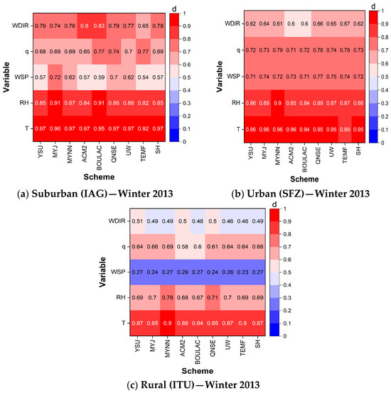
Figure 5.
Heatmap of the index of agreement d between hourly values of five conventional meteorological variables (T, RH, WSP, q, WDIR) modeled using WRF models with nine PBL schemes and observed at the surface in the (a) Suburban (IAG), (b) Urban (SFZ), and (c) Rural (ITU) areas of the MRSP over 10 consecutive days (6–15 August) in the winter of 2013.
3.2.2. Unconventional Variables (H, LE, RN, DSR)
Table A4 (Appendix B) shows the statistical parameters d, r, MBE, and RMSE estimated from four unconventional meteorological variables: H, LE, DSR, and RN, simulated by the WRF model with nine PBL schemes and observed at the suburban (IAG), urban (SFZ), and rural (ITU) areas of the MRSP during the winter field campaign of 2013.
In general, during the winter field campaign, the observed values of H and LE were overestimated by all PBL schemes (Table A4). Regarding H, the WRF model simulation performed best with the ACM2 scheme in the rural area (d = 0.96, r = 0.93, MBE = 13.40 W m−2, RMSE = 41.57 W m−2), followed by the BouLac scheme in the suburban area (d = 0.94, r = 0.90, MBE = 5.54 W m−2, RMSE = 34.32 W m−2), and the TEMF scheme in the urban area (d = 0.82, r = 0.69, MBE = −4.33 W m−2, RMSE = 46.88 W m−2). Except for the WRF model simulation of H with the TEMF scheme (MBE = −18.84 Wm−2) and the QNSE scheme (MBE = −1.01 Wm−2) in the suburban area, most of the PBL schemes yielded positive MBE, consistently overestimating the observed H in both areas of the MRSP during the winter field campaign.
In the case of H, the best performance was achieved by the BouLac scheme (d = 0.94, r = 0.90, MBE = 5.54 W m−2, RMSE = 34.32 W m−2) for the suburban area, followed by the UW scheme (d = 0.82, r = 0.69, MBE = −4.33 W m−2, RMSE = 46.88 W m−2) for the urban area, and by the ACM2 scheme (d = 0.96, r = 0.93, MBE = 13.40 W m−2, RMSE = 41.57 W m−2) for the rural area. In the case of LE, the best performance was achieved by the QNSE scheme (d = 0.91, r = 0.90, MBE = −13.66 W m−2, RMSE = 31.63 W m−2) for the rural area, followed by the YSU scheme (d = 0.70, r = 0.85, MBE = 23.56 W m−2, RMSE = 45.54 W m−2) for the suburban area, and by the MYNN scheme (d = 0.59, r = 0.45, MBE = 6.80 W m−2, RMSE = 22.31 W m−2) for the urban area.
For suburban, urban, and rural areas of the MRSP (Table A4), the WRF model simulations of DSR overestimated the observations by all parameterizations. Except for rural areas, RN simulations underestimated observations in the MRSP. High values of d and r indicated a high level of agreement between simulations of DSR and RN in all areas of the MRSP during the winter field campaign. In the case of DSR, the best performance was achieved by the BouLac scheme (d = 0.97, r = 0.96, MBE = 28.18 W m−2, RMSE = 86.75 W m−2) for the suburban area, followed by the MYNN scheme (d = 0.95, r = 0.95, MBE = 42.49 W m−2, RMSE = 109.26 W m−2) for the urban area, and by the MYNN scheme (d = 0.96, r = 0.94, MBE = 43.35 W m−2, RMSE = 103.49 W m−2) for the rural area. In the case of RN, the best performance was achieved by the BouLac scheme (d = 0.98, r = 0.96, MBE = 7.62 W m−2, RMSE = 57.15 m−2) for the suburban area, followed by the ACM2 scheme (d = 0.95, r = 0.95, MBE = 25.40 W m−2, R MSE = 85.88 W m−2) for the urban area, and by the MYNN scheme (d = 0.95, r = 0.95, MBE = −39.09 W m−2, RMSE = 81.38 W m−2) for the rural area.
Figure 6 shows the diurnal evolution of hourly average values of H and LE simulated by the WRF model with nine PBL schemes and observed in the suburban (IAG), urban (SFZ), and rural (ITU) areas of the MRSP, during the winter field campaign of 2013. During the winter field campaign, the observed diurnal evolution of H was well represented by all PBL schemes in the suburban and rural areas. However, the observed average values of H were overestimated in the urban area, with closer values simulated by the TEMF scheme. The observed diurnal evolution of LE was well represented by all schemes in the rural area. The observed LE was overestimated in suburban and urban areas, especially in the daytime. In the rural area, the observed LE was slightly underestimated.

Figure 6.
Diurnal evolution of average hourly values of H and LE simulated by the WRF model and observed (OBS) at the surface in the suburban (IAG), urban (SFZ), and rural (ITU) areas of the MRSP, over 10 consecutive days (6–15 August) in the winter of 2013. Vertical bars indicate statistical errors.
Figure 7 shows the diurnal evolution of hourly average values of DSR and RN simulated by the WRF model with nine PBL schemes and observed in the suburban (IAG), urban (SFZ), and rural (ITU) areas of the MRSP during the winter field campaign of 2013. During the winter field campaign, the diurnal evolution of observed DSR was overestimated by the respective modeled values by the WRF model with all the PBL schemes in the suburban, urban, and rural areas of the MRSP. Except for the rural area, simulated RN overestimated observations in the suburban and urban areas. In the rural region, the simulated values of RN underestimated observation but remained closer to the real values in comparison to the suburban and urban areas. The simulated and observed values of RN for urban and rural areas had similar magnitudes. The largest discrepancies between simulated and observed values of RN, among other factors, may be related to the fact that observations are representative of one point and WRF model simulations represent radiometric properties in an area of 0.6 by 0.6 km.

Figure 7.
Diurnal evolution of average hourly values of DSR and RN simulated by the WRF model and observed (OBS) at the surface in the suburban (IAG), urban (SFZ), and rural (ITU) areas of the MRSP over 10 consecutive days (6–15 August) in the winter field campaign of 2013. Vertical bars indicate statistical errors.
3.3. Summary of WRF Model Performance in the MRSP
Figure 8 summarizes the performance of the WRF model considering the impact of nine PBL turbulence parametrization schemes over nine (conventional and nonconventional) meteorological variables simulated by the WRF model during the 2013 summer and winter field campaigns carried out in the MRSP.

Figure 8.
Distribution of mean (Mean) and standard deviation (SD) values of d in terms of PBL schemes. The values of the mean and standard deviation of d are estimated for each of the nine PBL schemes based on the eight values of d for each meteorological variable simulated by the WRF model and observed on the surface in the suburban (IAG), urban (SFZ), and rural (ITU) areas of the MRSP over the summer and winter field campaigns of 2013.
In this figure, each mean value of d is plotted as a function of the PBL schemes used in this work. The information conveyed by the distribution of mean values of d in terms of the PBL scheme is visually enhanced by combining the color and diameter of each solid circle with the mean and standard deviation of d values for each PBL scheme. The standard deviation is a measure of the dispersion of the data around the mean—a low (high) standard deviation indicates less (more) variability thus the PBL scheme yielded simulated values closer (farther) to the observed values and will be plotted as small (large) diameter circle. On the other hand, in the case of d, values closer to 1 (0) indicate better (worse) agreement between the simulations and the observations and will be represented by darker (clearer) circles. Therefore, in Figure 8, the best performance of a given PBL scheme is identified by the smallest and darkest circles.
Therefore, the MYJ is the scheme that best represents the meteorological and topographical conditions of the MRSP. This suggests that the MYJ scheme was the most capable of reproducing the patterns observed on the surface of the MRSP during the summer and winter field campaign of 2013 compared to the other PBL parameterization schemes used in the WRF model.
In urban environments with complex geometry and variations in land use, MYJ can offer a more accurate representation of local conditions, considering the interaction between the urban surface and the surrounding atmosphere in contrast to non-local schemes, which represent more intense vertical mixing leading to a larger overestimation of urban WSP. MYJ produces a more balanced representation of vertical mixing, and consequently, a better estimate of the dynamic and thermodynamic characteristics of PBL on the surface of the MRSP.
4. Conclusions
The aim of this work was to determine which of the nine PBL turbulence parameterization schemes available in the WRF model is the most suitable for numerically simulating the temporal and spatial evolution of PBL properties, mainly surface conventional (T, HR, q, WSP, WDIR) and unconventional (H, LE, H, LE, RN, DSR) meteorological variables, measured at the surface in the suburban (IAG), urban (SFZ), and rural (ITU) areas of the MRSP over the summer (19–28 February) and winter (6–15 August) field campaigns of the MCITY BRAZIL project in 2013.
To this end, the high quality observed at the surface in three micrometeorological platforms (SFZ, IAG, and ITU), representative of urban, suburban, and rural land use of the MRSP, were used to estimate hourly values of T, HR, q, WSP, WDIR, H, LE, DSR, RN, and objectively compared with equivalent meteorological variables simulated with the WRF model using nine PBL turbulence parametrization schemes based on local closures of order 1.5 (MYNN, MYJ, QNSE, UW, BouLac), nonlocal closures of order 1.0 (YSU, SH), and hybrid closures of order 1.0 (ACM2) and 1.5 (TEMF).
During the summer field campaign, the simulations showed cold and dry bias, as well as an overestimation of wind speed. We detected an overestimation of H, but with high agreement and correlation values. The LE simulations performed well, with low MBE and RMSE values. DSR and RN were also well simulated. In this period, the local MYJ scheme performed best for the suburban area of the MRSP.
During the winter field campaign, the simulations showed very different behaviors depending on the land use of the site and meteorological variables. The MYJ, BouLac, and MYNN schemes performed well in simulating temperature and humidity, especially in the urban area of the MRSP. The MYNN scheme also performed well in simulating RN. There was a tendency for H and LE to be overestimated, except in the rural area, where they were consistently underestimated. However, simulations in the rural area showed the best correlations compared to the urban areas of the MRSP.
In general, the MYJ scheme was considered the most suitable for representing the meteorological and topographical conditions of the MRSP in contrast to non-local schemes that represent a more intense vertical mixing, leading to an overestimation of wind speed in the MRSP.
Author Contributions
Conceptualization, J.V.T. and A.P.d.O.; methodology, J.V.T. and M.P.S.; software, J.V.T.; formal analysis, J.V.T. and M.P.S.; investigation, J.V.T., A.P.d.O., M.P.S., J.V.T., and A.F.; resources, A.P.d.O.; data curation, J.V.T. and M.P.S. All authors have read and agreed to the published version of the manuscript.
Funding
This research was sponsored by the National Council for Scientific and Technological Development (CNPq): 304786/2018-7, 166519/2017-0, 309079/2013-6; 305357/2012-3, 462734/2014-5; the São Paulo Research Foundation (FAPESP): FAPESP (2020/07141-2, 2011/50178-5), FAPERJ (E26/111.620/2011, E-26/103.407/2012).
Institutional Review Board Statement
Not applicable.
Informed Consent Statement
Not applicable.
Data Availability Statement
The original contributions presented in the study are included in the article, further inquiries can be directed to the corresponding author.
Conflicts of Interest
The authors declare no conflicts of interest.
Appendix A
Table A1.
Statistical parameters (d, r, MBE, RMSE) estimated from N pairs of hourly values of the conventional variables (T, RH, q, WSP, WDIR), simulated using the WRF model (with nine PBL schemes) and measured at the surface of the Suburban (IAG) area in the MRSP and over 10 days in the summer field campaign of 2013 (19–28 February). Best (worst) statistical parameter values are indicated by black (red) boldface numbers and light blueish (reddish) table-cell colors.
| Statistical Parameters—Summer Field Campaign of 2013 (19–28 February) | |||||
|---|---|---|---|---|---|
| Conventional Variable | PBL Scheme | Suburban (IAG) | |||
| T (°C) | d | r | MBE (°C) | RMSE (°C) | |
| YSU | 0.91 | 0.87 | −0.65 | 1.91 | |
| MYJ | 0.94 | 0.89 | −0.27 | 1.68 | |
| MYNN | 0.90 | 0.87 | −0.83 | 2.00 | |
| ACM2 | 0.93 | 0.88 | 0.05 | 1.74 | |
| BouLac | 0.94 | 0.90 | 0.04 | 1.62 | |
| QNSE | 0.88 | 0.87 | −1.21 | 2.17 | |
| UW | 0.91 | 0.87 | −0.63 | 1.93 | |
| TEMF | 0.62 | 0.56 | −3.95 | 5.19 | |
| SH | 0.93 | 0.91 | −0.33 | 1.61 | |
| RH (%) | d | r | MBE (%) | RMSE (%) | |
| YSU | 0.84 | 0.75 | −2.25 | 10.57 | |
| MYJ | 0.90 | 0.85 | −3.75 | 9.11 | |
| MYNN | 0.84 | 0.76 | −6.30 | 12.24 | |
| ACM2 | 0.83 | 0.77 | −7.66 | 12.81 | |
| BouLac | 0.85 | 0.78 | −4.81 | 10.78 | |
| QNSE | 0.85 | 0.77 | −0.48 | 9.98 | |
| UW | 0.85 | 0.75 | −2.75 | 10.60 | |
| TEMF | 0.60 | 0.54 | −8.29 | 19.60 | |
| SH | 0.87 | 0.80 | −3.60 | 9.99 | |
| q (g kg−1) | d | r | MBE (g kg−1) | RMSE (g kg−1) | |
| YSU | 0.61 | 0.49 | −0.90 | 1.53 | |
| MYJ | 0.64 | 0.53 | −0.94 | 1.43 | |
| MYNN | 0.45 | 0.28 | −1.90 | 2.53 | |
| ACM2 | 0.47 | 0.24 | −1.48 | 2.13 | |
| BouLac | 0.58 | 0.37 | −0.82 | 1.53 | |
| QNSE | 0.52 | 0.31 | −1.00 | 1.69 | |
| UW | 0.57 | 0.42 | −1.01 | 1.58 | |
| TEMF | 0.36 | 0.31 | −1.88 | 2.59 | |
| SH | 0.64 | 0.53 | −0.91 | 1.46 | |
| WSP (m s−1) | d | r | MBE (m s−1) | RMSE (m s−1) | |
| YSU | 0.56 | 0.59 | 1.70 | 2.21 | |
| MYJ | 0.70 | 0.64 | 0.85 | 1.52 | |
| MYNN | 0.57 | 0.52 | 1.44 | 1.99 | |
| ACM2 | 0.55 | 0.59 | 1.82 | 2.28 | |
| BouLac | 0.53 | 0.51 | 1.70 | 2.26 | |
| QNSE | 0.62 | 0.61 | 1.30 | 1.83 | |
| UW | 0.57 | 0.56 | 1.49 | 2.18 | |
| TEMF | 0.37 | 0.35 | 1.66 | 2.70 | |
| SH | 0.55 | 0.52 | 1.63 | 2.14 | |
| WDIR (°) | d | r | MBE (°) | RMSE (°) | |
| YSU | 0.62 | 0.51 | −1.36 | 20.65 | |
| MYJ | 0.70 | 0.68 | 1.38 | 20.94 | |
| MYNN | 0.65 | 0.55 | −0.51 | 7.77 | |
| ACM2 | 0.67 | 0.57 | 10.59 | 160.27 | |
| BouLac | 0.68 | 0.62 | 8.11 | 122.79 | |
| QNSE | 0.68 | 0.63 | −0.13 | 2.04 | |
| UW | 0.66 | 0.60 | −2.66 | 40.25 | |
| TEMF | 0.45 | 0.23 | 11.54 | 174.61 | |
| SH | 0.68 | 0.65 | −1.94 | 29.38 | |
Table A2.
Statistical parameters (d, r, MBE, RMSE) estimated from N pairs of hourly values of the unconventional variables (H, LE, RN, DSR), simulated using the WRF model (with nine PBL schemes) and measured at the surface of the IAG (suburban) in the MRSP and over 10 days in the summer field campaign of 2013 (19–28 February). Best (worst) statistical parameter values are indicated by black (red) boldface numbers and light blueish (reddish) table-cell colors.
| Statistical Parameters—Summer Field Campaign of 2013 (19–28 February) | |||||
|---|---|---|---|---|---|
| Unconventional Variable | PBL Scheme | Suburban (IAG) | |||
| d | r | MBE (W m−2) | RMSE (W m−2) | ||
| H (W m−2) | YSU | 0.84 | 0.83 | 38.48 | 70.20 |
| MYJ | 0.86 | 0.87 | 42.63 | 66.54 | |
| MYNN | 0.93 | 0.83 | 12.80 | 40.07 | |
| ACM2 | 0.89 | 0.86 | 28.41 | 54.46 | |
| BouLac | 0.89 | 0.89 | 36.66 | 59.32 | |
| QNSE | 0.90 | 0.90 | 33.99 | 55.64 | |
| UW | 0.89 | 0.88 | 33.03 | 56.21 | |
| TEMF | 0.65 | 0.43 | −44.35 | 89.10 | |
| SH | 0.88 | 0.88 | 37.60 | 61.08 | |
| LE (W m−2) | YSU | 0.91 | 0.86 | −0.55 | 41.49 |
| MYJ | 0.91 | 0.85 | 1.94 | 42.57 | |
| MYNN | 0.89 | 0.81 | −6.40 | 42.68 | |
| ACM2 | 0.90 | 0.83 | −4.32 | 42.09 | |
| BouLac | 0.93 | 0.88 | 1.08 | 37.23 | |
| QNSE | 0.90 | 0.86 | 12.64 | 47.26 | |
| UW | 0.92 | 0.86 | −1.32 | 39.86 | |
| TEMF | 0.78 | 0.65 | −27.12 | 62.44 | |
| SH | 0.91 | 0.85 | −1.19 | 40.45 | |
| DSR (W m−2) | YSU | 0.92 | 0.86 | 42.55 | 198.75 |
| MYJ | 0.93 | 0.90 | 68.42 | 186.70 | |
| MYNN | 0.94 | 0.88 | −1.65 | 156.28 | |
| ACM2 | 0.94 | 0.88 | 30.55 | 166.70 | |
| BouLac | 0.94 | 0.89 | 38.28 | 171.90 | |
| QNSE | 0.94 | 0.90 | 53.60 | 174.85 | |
| UW | 0.94 | 0.89 | 34.57 | 173.69 | |
| TEMF | 0.84 | 0.57 | 88.37 | 205.19 | |
| SH | 0.94 | 0.91 | 51.06 | 165.77 | |
| RN (W m−2) | YSU | 0.91 | 0.84 | 18.09 | 156.55 |
| MYJ | 0.93 | 0.89 | 41.74 | 145.75 | |
| MYNN | 0.93 | 0.86 | −3.84 | 132.11 | |
| ACM2 | 0.93 | 0.86 | 6.63 | 136.97 | |
| BouLac | 0.93 | 0.87 | 14.11 | 136.85 | |
| QNSE | 0.93 | 0.89 | 39.56 | 144.38 | |
| UW | 0.93 | 0.87 | 14.10 | 139.57 | |
| TEMF | 0.75 | 0.59 | −83.81 | 229.26 | |
| SH | 0.94 | 0.89 | 21.42 | 133.54 | |
Appendix B
Table A3.
Statistical parameters (d, r, MBE, RMSE) estimated from N pairs of hourly values of the conventional variables (T, RH, q, WSP, WDIR), simulated using the WRF model (with nine PBL schemes) and measured at the surface of the suburban (IAG), urban (SFZ), and rural (ITU) in the MRSP and over 10 days in the winter field campaign of 2013 (6–15 August). Best (worst) statistical parameter values are indicated by black (red) boldface numbers and light blueish (reddish) table-cell colors.
| Statistical Parameters—Winter Field Campaign of 2013 (6–15 August) | |||||||||||||
|---|---|---|---|---|---|---|---|---|---|---|---|---|---|
| Conventional Variable | PBL Scheme | ||||||||||||
| Suburban (IAG) | Urban (SFZ) | Rural (ITU) | |||||||||||
| T (°C) | d | r | MBE (°C) | RMSE (°C) | d | r | MBE (°C) | RMSE (°C) | d | r | MBE (°C) | RMSE (°C) | |
| YSU | 0.97 | 0.95 | 0.43 | 1.75 | 0.96 | 0.95 | 1.40 | 2.26 | 0.87 | 0.86 | 2.64 | 3.92 | |
| MYJ | 0.96 | 0.93 | −0.56 | 2.07 | 0.96 | 0.93 | 0.64 | 2.17 | 0.85 | 0.83 | 2.71 | 4.24 | |
| MYNN | 0.97 | 0.94 | −0.16 | 1.84 | 0.96 | 0.92 | 0.06 | 2.09 | 0.90 | 0.88 | 1.68 | 3.22 | |
| ACM2 | 0.97 | 0.95 | 0.35 | 1.73 | 0.96 | 0.95 | 1.33 | 2.21 | 0.88 | 0.88 | 2.67 | 3.83 | |
| BouLac | 0.95 | 0.94 | −0.86 | 2.13 | 0.94 | 0.94 | 1.97 | 2.69 | 0.84 | 0.83 | 3.13 | 4.47 | |
| QNSE | 0.97 | 0.95 | 0.20 | 1.83 | 0.95 | 0.93 | 1.09 | 2.25 | 0.85 | 0.85 | 2.96 | 4.19 | |
| UW | 0.97 | 0.95 | 0.33 | 1.73 | 0.95 | 0.94 | 1.37 | 2.28 | 0.87 | 0.85 | 2.71 | 4.05 | |
| TEMF | 0.92 | 0.89 | 1.43 | 2.95 | 0.89 | 0.88 | 2.41 | 3.57 | 0.80 | 0.82 | 3.94 | 5.19 | |
| SH | 0.97 | 0.95 | 0.46 | 1.82 | 0.95 | 0.94 | 1.42 | 2.29 | 0.87 | 0.85 | 2.53 | 3.93 | |
| RH (%) | d | r | MBE (%) | RMSE (%) | d | r | MBE (%) | RMSE (%) | d | r | MBE (%) | RMSE (%) | |
| YSU | 0.85 | 0.81 | −8.79 | 14.77 | 0.86 | 0.80 | −8.19 | 15.38 | 0.69 | 0.62 | −17.06 | 24.55 | |
| MYJ | 0.91 | 0.85 | −3.98 | 10.98 | 0.89 | 0.81 | −4.13 | 12.75 | 0.70 | 0.59 | −15.09 | 23.25 | |
| MYNN | 0.87 | 0.82 | −7.59 | 13.60 | 0.90 | 0.82 | −2.30 | 11.42 | 0.78 | 0.71 | −11.94 | 18.54 | |
| ACM2 | 0.84 | 0.83 | −10.63 | 15.62 | 0.85 | 0.82 | −9.67 | 15.76 | 0.68 | 0.65 | −19.39 | 26.04 | |
| BouLac | 0.91 | 0.84 | −2.70 | 10.05 | 0.84 | 0.80 | −9.70 | 15.97 | 0.67 | 0.57 | −17.71 | 26.16 | |
| QNSE | 0.88 | 0.83 | −6.50 | 12.48 | 0.89 | 0.82 | −5.63 | 13.14 | 0.71 | 0.65 | −16.45 | 23.45 | |
| UW | 0.88 | 0.84 | −7.95 | 13.39 | 0.87 | 0.81 | −7.33 | 14.31 | 0.70 | 0.62 | −15.77 | 23.69 | |
| TEMF | 0.82 | 0.73 | −7.66 | 15.62 | 0.87 | 0.78 | −4.63 | 13.85 | 0.69 | 0.57 | −13.93 | 23.59 | |
| SH | 0.85 | 0.82 | −9.41 | 14.84 | 0.86 | 0.81 | −8.60 | 15.17 | 0.69 | 0.60 | −16.67 | 24.66 | |
| q (g kg−1) | d | r | MBE (g kg−1) | RMSE (g kg−1) | d | r | MBE (g kg−1) | RMSE (g kg−1) | d | r | MBE (g kg−1) | RMSE (g kg−1) | |
| YSU | 0.68 | 0.57 | −1.13 | 1.81 | 0.72 | 0.54 | −0.62 | 1.53 | 0.64 | 0.43 | −0.70 | 1.96 | |
| MYJ | 0.69 | 0.54 | −0.95 | 1.74 | 0.73 | 0.55 | −0.37 | 1.45 | 0.66 | 0.48 | −0.37 | 1.77 | |
| MYNN | 0.69 | 0.59 | −1.22 | 1.83 | 0.79 | 0.63 | −0.33 | 1.31 | 0.69 | 0.52 | −0.47 | 1.74 | |
| ACM2 | 0.65 | 0.58 | −1.44 | 1.99 | 0.71 | 0.55 | −0.87 | 1.63 | 0.58 | 0.33 | −1.04 | 2.20 | |
| BouLac | 0.77 | 0.68 | −0.84 | 1.48 | 0.72 | 0.52 | −0.51 | 1.54 | 0.60 | 0.38 | −0.57 | 1.97 | |
| QNSE | 0.74 | 0.62 | −0.86 | 1.60 | 0.78 | 0.62 | −0.35 | 1.33 | 0.61 | 0.39 | −0.42 | 1.90 | |
| UW | 0.70 | 0.60 | −1.06 | 1.70 | 0.74 | 0.58 | −0.49 | 1.42 | 0.64 | 0.44 | −0.53 | 1.86 | |
| TEMF | 0.77 | 0.63 | −0.31 | 1.62 | 0.78 | 0.67 | 0.54 | 1.52 | 0.64 | 0.41 | 0.48 | 2.02 | |
| SH | 0.69 | 0.59 | −1.17 | 1.81 | 0.73 | 0.56 | −0.64 | 1.51 | 0.66 | 0.45 | −0.71 | 1.93 | |
| WSP (m s−1) | d | r | MBE (m s−1) | RMSE (m s−1) | d | r | MBE (m s−1) | RMSE (m s−1) | d | r | MBE (m s−1) | RMSE (m s−1) | |
| SU | 0.57 | 0.57 | 1.92 | 2.68 | 0.71 | 0.58 | 0.67 | 2.28 | 0.27 | 0.39 | 3.78 | 4.24 | |
| MYJ | 0.72 | 0.70 | 0.99 | 1.89 | 0.74 | 0.57 | −0.30 | 2.10 | 0.24 | 0.34 | 4.24 | 4.75 | |
| MYNN | 0.62 | 0.67 | 1.77 | 2.44 | 0.72 | 0.54 | 0.35 | 2.07 | 0.27 | 0.46 | 4.30 | 4.70 | |
| ACM2 | 0.57 | 0.60 | 2.08 | 2.71 | 0.73 | 0.59 | 0.71 | 2.17 | 0.29 | 0.52 | 3.99 | 4.38 | |
| BouLac | 0.59 | 0.57 | 1.81 | 2.47 | 0.71 | 0.58 | 0.84 | 2.28 | 0.27 | 0.39 | 3.76 | 4.25 | |
| QNSE | 0.70 | 0.70 | 1.22 | 1.99 | 0.77 | 0.63 | −0.04 | 1.90 | 0.24 | 0.38 | 4.54 | 5.00 | |
| UW | 0.62 | 0.65 | 1.70 | 2.42 | 0.75 | 0.64 | 0.52 | 2.12 | 0.26 | 0.34 | 3.72 | 4.24 | |
| TEMF | 0.54 | 0.53 | 1.64 | 2.72 | 0.74 | 0.58 | −0.20 | 1.89 | 0.23 | 0.28 | 4.43 | 5.06 | |
| SH | 0.57 | 0.57 | 1.94 | 2.68 | 0.72 | 0.58 | 0.65 | 2.23 | 0.27 | 0.39 | 3.74 | 4.22 | |
| WDIR (°) | d | r | MBE (°) | RMSE (°) | d | r | MBE (°) | RMSE (°) | d | r | MBE (°) | RMSE (°) | |
| YSU | 0.76 | 0.57 | −8.55 | 136.00 | 0.62 | 0.51 | −19.23 | 126.01 | 0.51 | 0.23 | −14.58 | 141.22 | |
| MYJ | 0.74 | 0.56 | −7.74 | 123.05 | 0.64 | 0.57 | −21.87 | 125.70 | 0.49 | 0.21 | −15.36 | 138.63 | |
| MYNN | 0.76 | 0.52 | −3.36 | 53.43 | 0.61 | 0.52 | −18.57 | 123.99 | 0.49 | 0.17 | −12.97 | 139.14 | |
| ACM2 | 0.80 | 0.74 | −6.91 | 109.92 | 0.60 | 0.45 | −19.89 | 125.58 | 0.50 | 0.18 | −14.06 | 138.07 | |
| BouLac | 0.83 | 0.65 | −7.45 | 118.42 | 0.60 | 0.51 | −16.64 | 126.98 | 0.48 | 0.16 | −14.17 | 144.85 | |
| QNSE | 0.79 | 0.73 | −10.48 | 166.77 | 0.66 | 0.56 | −23.53 | 124.25 | 0.50 | 0.21 | −20.49 | 136.75 | |
| UW | 0.77 | 0.71 | −6.28 | 99.91 | 0.65 | 0.55 | −19.42 | 125.19 | 0.46 | 0.10 | −10.07 | 144.88 | |
| TEMF | 0.65 | 0.49 | 3.80 | 60.42 | 0.67 | 0.56 | −17.41 | 128.81 | 0.46 | 0.22 | −3.61 | 152.73 | |
| SH | 0.78 | 0.66 | −7.33 | 116.67 | 0.62 | 0.53 | −19.03 | 126.89 | 0.49 | 0.19 | −13.36 | 140.56 | |
Table A4.
Statistical parameters (d, r, MBE, RMSE) estimated from N pairs of hourly values of the unconventional variables (H, LE, RN, DSR), simulated using the WRF model (with nine PBL schemes) and measured at the surface of the suburban (IAG), urban (SFZ), and rural (ITU) in the MRSP and over 10 days in the winter field campaign of 2013 (6–15 August). Best (worst) statistical parameter values are indicated by black (red) boldface numbers and light blueish (reddish) table-cell colors.
| Statistical Parameter—Winter Field Campaign of 2013 (6–15 August) | |||||||||||||
|---|---|---|---|---|---|---|---|---|---|---|---|---|---|
| Unconventional Variable | PBL Scheme | Suburban (IAG) | Urban (SFZ) | Rural (ITU) | |||||||||
| d | r | MBE (Wm−2) | RMSE (Wm−2) | d | r | MBE (Wm−2) | RMSE (Wm−2) | d | r | MBE (W m−2) | RMSE (W m−2) | ||
| c (W m−2) | YSU | 0.93 | 0.87 | 6.11 | 37.83 | 0.79 | 0.68 | 8.09 | 56.62 | 0.95 | 0.92 | 16.15 | 46.07 |
| MYJ | 0.93 | 0.87 | 9.65 | 38.66 | 0.79 | 0.67 | 9.33 | 56.29 | 0.94 | 0.91 | 26.25 | 55.86 | |
| MYNN | 0.93 | 0.88 | 1.20 | 36.15 | 0.76 | 0.65 | 8.64 | 60.26 | 0.94 | 0.92 | 28.22 | 54.69 | |
| ACM2 | 0.94 | 0.89 | 4.63 | 34.26 | 0.76 | 0.65 | 7.32 | 59.78 | 0.96 | 0.93 | 13.40 | 41.57 | |
| BouLac | 0.94 | 0.90 | 5.54 | 34.32 | 0.78 | 0.67 | 7.20 | 57.32 | 0.94 | 0.91 | 14.38 | 47.95 | |
| QNSE | 0.94 | 0.88 | −1.01 | 34.89 | 0.80 | 0.69 | 5.91 | 53.15 | 0.94 | 0.92 | 27.11 | 58.37 | |
| UW | 0.94 | 0.89 | 6.19 | 34.81 | 0.76 | 0.65 | 10.68 | 60.32 | 0.95 | 0.91 | 13.20 | 46.24 | |
| TEMF | 0.85 | 0.82 | −18.84 | 47.59 | 0.82 | 0.69 | −4.33 | 46.88 | 0.93 | 0.88 | 14.51 | 53.88 | |
| SH | 0.94 | 0.88 | 6.05 | 36.64 | 0.79 | 0.69 | 8.00 | 56.31 | 0.95 | 0.91 | 16.25 | 47.99 | |
| LE (W m−2) | YSU | 0.70 | 0.85 | 23.56 | 45.54 | 0.58 | 0.42 | 6.40 | 22.21 | 0.88 | 0.91 | −20.77 | 35.93 |
| MYJ | 0.68 | 0.85 | 26.50 | 50.03 | 0.58 | 0.44 | 7.64 | 23.57 | 0.88 | 0.90 | −18.97 | 35.51 | |
| MYNN | 0.65 | 0.84 | 29.47 | 54.15 | 0.59 | 0.45 | 6.80 | 22.31 | 0.88 | 0.92 | −19.77 | 35.18 | |
| ACM2 | 0.69 | 0.84 | 25.29 | 48.01 | 0.58 | 0.43 | 6.65 | 22.63 | 0.89 | 0.90 | −18.89 | 35.24 | |
| BouLac | 0.68 | 0.83 | 25.17 | 48.39 | 0.58 | 0.44 | 7.48 | 22.84 | 0.89 | 0.90 | −18.15 | 34.81 | |
| QNSE | 0.62 | 0.85 | 33.77 | 59.04 | 0.53 | 0.44 | 11.00 | 27.31 | 0.91 | 0.90 | −13.66 | 31.63 | |
| UW | 0.70 | 0.85 | 23.73 | 46.06 | 0.58 | 0.43 | 6.61 | 22.48 | 0.87 | 0.90 | −20.82 | 36.83 | |
| TEMF | 0.56 | 0.78 | 37.95 | 67.83 | 0.47 | 0.39 | 12.81 | 29.42 | 0.89 | 0.88 | −13.44 | 34.30 | |
| SH | 0.70 | 0.85 | 24.54 | 46.28 | 0.58 | 0.43 | 6.48 | 22.12 | 0.88 | 0.91 | −20.55 | 35.96 | |
| d | r | MBE (W m−2) | RMSE (W m−2) | d | r | MBE (W m−2) | RMSE (W m−2) | d | r | MBE (W m−2) | RMSE (W m−2) | ||
| DSR (W m−2) | YSU | 0.96 | 0.95 | 44.92 | 109.38 | 0.94 | 0.94 | 62.50 | 130.03 | 0.92 | 0.89 | 64.34 | 147.29 |
| MYJ | 0.96 | 0.95 | 47.95 | 111.33 | 0.94 | 0.94 | 61.82 | 130.89 | 0.92 | 0.89 | 63.03 | 149.32 | |
| MYNN | 0.97 | 0.95 | 35.53 | 98.80 | 0.95 | 0.95 | 42.49 | 109.26 | 0.96 | 0.94 | 43.35 | 103.49 | |
| ACM2 | 0.96 | 0.96 | 43.26 | 100.19 | 0.95 | 0.95 | 58.82 | 118.65 | 0.93 | 0.90 | 59.64 | 140.09 | |
| BouLac | 0.97 | 0.96 | 28.18 | 86.75 | 0.93 | 0.94 | 64.14 | 132.48 | 0.90 | 0.85 | 67.26 | 168.77 | |
| QNSE | 0.96 | 0.95 | 45.86 | 108.84 | 0.93 | 0.94 | 62.72 | 131.68 | 0.90 | 0.86 | 66.90 | 164.91 | |
| UW | 0.96 | 0.95 | 46.84 | 109.98 | 0.93 | 0.94 | 63.97 | 134.24 | 0.90 | - | 64.46 | 169.75 | |
| TEMF | 0.93 | 0.88 | 19.56 | 133.11 | 0.91 | 0.87 | 39.53 | 147.39 | 0.90 | 0.84 | 66.46 | 169.76 | |
| SH | 0.97 | 0.96 | 44.48 | 100.36 | 0.94 | 0.94 | 60.98 | 130.99 | 0.93 | 0.90 | 59.58 | 141.97 | |
| RN (W m−2) | YSU | 0.97 | 0.95 | 10.16 | 68.05 | 0.94 | 0.94 | 31.30 | 91.86 | 0.93 | 0.91 | −31.84 | 90.44 |
| MYJ | 0.97 | 0.95 | 21.14 | 73.06 | 0.93 | 0.94 | 39.96 | 99.94 | 0.94 | 0.90 | −28.35 | 90.17 | |
| MYNN | 0.97 | 0.96 | 7.11 | 66.44 | 0.94 | 0.94 | 28.71 | 87.45 | 0.95 | 0.95 | −39.09 | 81.38 | |
| ACM2 | 0.98 | 0.96 | 4.83 | 62.82 | 0.95 | 0.95 | 25.40 | 85.88 | 0.94 | 0.92 | −37.71 | 89.15 | |
| BouLac | 0.98 | 0.96 | 7.62 | 57.15 | 0.94 | 0.94 | 32.81 | 92.48 | 0.93 | 0.89 | −28.35 | 95.23 | |
| QNSE | 0.97 | 0.95 | 22.45 | 76.20 | 0.93 | 0.94 | 44.31 | 104.71 | 0.94 | 0.90 | −23.58 | 91.03 | |
| UW | 0.97 | 0.95 | 9.85 | 70.62 | 0.94 | 0.93 | 31.31 | 95.98 | 0.93 | - | −36.00 | 93.07 | |
| TEMF | 0.94 | 0.89 | 0.62 | 96.13 | 0.91 | 0.87 | 25.47 | 113.27 | 0.92 | 0.87 | −22.67 | 100.10 | |
| SH | 0.98 | 0.96 | 8.42 | 63.29 | 0.94 | 0.94 | 30.03 | 92.51 | 0.93 | 0.92 | −35.78 | 90.66 | |
References
- Stull, R.B. An Introduction to Boundary Layer Meteorology; Kluwer Academic Publishers: Dordrecht, The Netherlands, 1988; 666p. [Google Scholar]
- Stensrud, D.J. Parameterization Schemes: Keys to Understanding Numerical Weather Prediction Models; Cambridge University Press: Cambridge, UK, 2007; 459p. [Google Scholar]
- Braun, S.A.; Tao, W.-K. Sensitivity of High-Resolution Simulations of Hurricane Bob (1991) to Planetary Boundary Layer Parameterizations. Mon. Weather Rev. 2000, 128, 3941–3961. [Google Scholar] [CrossRef]
- Li, X.; Pu, Z. Sensitivity of Numerical Simulation of Early Rapid Intensification of Hurricane Emily (2005) to Cloud Microphysical and Planetary Boundary Layer Parameterizations. Mon. Weather Rev. 2008, 136, 4819–4838. [Google Scholar] [CrossRef]
- Cohen, A.E.; Cavallo, S.M.; Coniglio, M.C.; Brooks, H.E. A Review of Planetary Boundary Layer Parameterization Schemes and Their Sensitivity in Simulating Southeastern U.S. Cold Season Severe Weather Environments. Weather Forecast. 2015, 30, 591–612. [Google Scholar] [CrossRef]
- Seaman, N.L. Meteorological modeling for air-quality assessments. Atmos. Environ. 2000, 34, 2231–2259. [Google Scholar] [CrossRef]
- Bossioli, E.; Tombrou, M.; Dandou, A.; Athanasopoulou, E.; Varotsos, K.V. The Role of Planetary Boundary-Layer Parameterizations in the Air Quality of an Urban Area with Complex Topography. Bound.-Layer Meteorol. 2009, 131, 53–72. [Google Scholar] [CrossRef]
- Banks, R.F.; Tiana-Alsina, J.; Baldasano, J.M.; Rocadenbosch, F.; Papayannis, A.; Solomos, S.; Tzanis, C.G. Sensitivity of boundary-layer variables to PBL schemes in the WRF model based on surface meteorological observations, lidar, and radiosondes during the HygrA-CD campaign. Atmos. Res. 2016, 176–177, 185–201. [Google Scholar] [CrossRef]
- Avolio, E.; Federico, S.; Migliettac, M.; Lo Feudo, T.; Calidonnaa, C.R.; Semprevivad, A.M. Sensitivity analysis of WRF model PBL schemes in simulating boundary-layer variables in southern Italy: An experimental campaign. Atmos. Res. 2017, 192, 58–71. [Google Scholar] [CrossRef]
- Holton, J.R. Introduction to Dynamic Meteorology, 4th ed.; Elsevier: Amsterdam, The Netherlands, 2004; p. 535. [Google Scholar]
- Cheng, F.; Chin, S.C.; Liu, T.H. The role of boundary layer schemes in meteorological and air quality simulations of the Taiwan area. Atmos. Environ. 2012, 54, 714–727. [Google Scholar] [CrossRef]
- Wang, W.; Shen, X.; Huang, W. A Comparison of Boundary-Layer Characteristics Simulated Using Different Parametrization Schemes. Bound.-Layer Meteorol. 2016, 161, 375–403. [Google Scholar] [CrossRef]
- Jia, W.; Zhang, X. The role of the planetary boundary layer parameterization schemes on the meteorological and aerosol pollution simulations: A review. Atmos. Res. 2020, 239, 104890. [Google Scholar] [CrossRef]
- Banks, R.F.; Tiana-Alsina, J.; Rocadenbosch, F.; Baldasano, J.M. Performance Evaluation of the Boundary-Layer Height from Lidar and the Weather Research and Forecasting Model at an Urban Coastal Site in the North-East Iberian Peninsula. Bound.-Layer Meteorol. 2015, 157, 265–292. [Google Scholar] [CrossRef]
- Boadh, R.; Satyanarayana, A.N.V.; Rama Krishna, T.V.B.P.S.; Madala, S. Sensitivity of PBL schemes of the WRF-ARW model in simulating the boundary layer flow parameters for its application to air pollution dispersion modeling over a tropical station. Atmosfera 2016, 29, 61–81. [Google Scholar]
- Sathyanadh, A.; Prabhab, T.V.; Balajib, B.; Resmib, E.A.; Karipot, A. Evaluation of WRF PBL parameterization schemes against direct observations during a dry event over the Ganges valley. Atmos. Res. 2017, 193, 125–141. [Google Scholar] [CrossRef]
- Imran, H.M.; Kala, J.; Ng, A.W.M.; Muthukumaran, S. An evaluation of the performance of a WRF multi-physics ensemble for heatwave events over the city of Melbourne in southeast Australia. Clim. Dyn. 2018, 50, 2553–2586. [Google Scholar] [CrossRef]
- Wang, J.; Hu, X.M. Evaluating the performance of WRF urban schemes and PBL schemes over Dallas Fort Worth during a dry summer and a wet summer. J. Appl. Meteorol. Clim. 2021, 60, 779–798. [Google Scholar] [CrossRef]
- Hu, X.M.; Nielsen-Gammon, J.W.; Zhang, F. Evaluation of Three Planetary Boundary Layer Schemes in the WRF Model. J. Appl. Meteorol. Clim. 2010, 49, 1831–1844. [Google Scholar] [CrossRef]
- Shin, H.H.; Hong, S.-Y. Intercomparison of Planetary Boundary-Layer Parametrizations in the WRF Model for a Single Day from CASES-99. Bound.-Layer Meteorol. 2011, 139, 261–281. [Google Scholar] [CrossRef]
- Coniglio, M.C.; Correia, J., Jr.; Marsh, P.T.; Kong, F. Verification of convection-allowing WRF Model forecasts of the planetary boundary layer using sounding observations. Weather Forecast. 2013, 28, 842–862. [Google Scholar] [CrossRef]
- Kim, Y.; Sartelet, K.; Raut, J.C.; Chazette, P. Evaluation of the Weather Research and Forecast/Urban Model Over Greater Paris. Bound.-Layer Meteorol. 2013, 149, 105–132. [Google Scholar] [CrossRef]
- Draxl, C.; Hahmann, A.N.; Peña, A.; Giebel, G. Evaluating winds and vertical wind shear from Weather Research and Forecasting model forecasts using seven planetary boundary layer schemes. Wind Energy 2014, 17, 39–55. [Google Scholar] [CrossRef]
- Ferrero, E.; Vandenberghe, F.; Alessandrini, S.; Mortarini, L. Comparison of WRF PBL models in low-wind speed conditions against measured data. In Air Pollution Modeling and Its Application XXV; Springer International Publishing: Cham, Switzerland, 2018; Volume 35, pp. 129–134. [Google Scholar]
- Tyagi, B.; Magliulo, V.; Finardi, S.; Gasbarra, D.; Carlucci, P.; Toscano, P.; Zaldei, A.; Riccio, A.; Calori, G.; D’allura, A.; et al. Performance Analysis of Planetary Boundary Layer Parameterization Schemes in WRF Modeling Set Up over Southern Italy. Atmosphere 2018, 9, 272. [Google Scholar] [CrossRef]
- Hu, X.-M.; Ma, Z.; Lin, W.; Zhang, H.; Hu, J.; Wang, Y.; Xu, X.; Fuentes, J.D.; Xue, M. Impact of the Loess Plateau on the atmospheric boundary layer structure and air quality in the North China Plain: A case study. Sci. Total. Environ. 2014, 499, 228–237. [Google Scholar] [CrossRef] [PubMed]
- Penchah, M.; Malakooti, H.; Satkin, M. Evaluation of planetary boundary layer simulations for wind resource study in east of Iran. Renew. Energy 2017, 111, 1–10. [Google Scholar] [CrossRef]
- Tymvios, F.; Charalambous, D.; Michaelides, S.; Lelieveld, J. Intercomparison of boundary layer parameterizations for summer conditions in the eastern Mediterranean island of Cyprus using the WRF–ARW model. Atmos. Res. 2017, 208, 45–59. [Google Scholar] [CrossRef]
- Huang, M.; Gao, Z.; Miao, S.; Chen, F. Sensitivity of urban boundary layer simulation to urban canopy models and PBL schemes in Beijing. Meteorog. Atmos. Phys. 2019, 131, 1235–1248. [Google Scholar] [CrossRef]
- Oliveira, A.P.; Marques Filho, E.P.; Ferreira, M.J.; Codato, G.; Ribeiro, F.N.D.; Landulfo, E.; Moreira, G.A.; Pereira, M.M.R.; Mlakar, P.; Boznar, M.Z.; et al. Assessing urban effects on the climate of metropolitan regions of Brazil–Preliminary results of the MCITY BRAZIL project. Explor. Environ. Sci. Res. 2020, 1, 38–77. [Google Scholar] [CrossRef]
- IBGE. Demographics Censuses. Available online: http://www.ibge.gov.br/english/ (accessed on 20 April 2024).
- Alvares, C.A.; Stape, J.L.; Sentelhas, P.C.; De Moraes Gonçalves, J.L.; Sparovek, G. Köppen’s climate classification map for Brazil. Meteorol. Z. 2014, 22, 711–728. [Google Scholar] [CrossRef] [PubMed]
- Sánchez, M.P.; Oliveira, A.P.; Varona, R.P.; Tito, J.V.; Codato, G.; Ribeiro, F.N.D.; Marques Filho, E.P.; Silveira, L.C. Radiosonde based analysis of the urban boundary layer in the metropolitan region of São Paulo, Brazil. Earth Space Sci. 2020, 7, e2019EA000781. [Google Scholar] [CrossRef]
- Oliveira, A.P.; Bornstein, R.D.; Soares, J. Annual and Diurnal Wind Patterns in the City of São Paulo. Water Air Soil Pollut. Focus 2003, 3, 3–15. [Google Scholar] [CrossRef]
- Sánchez, M.P.; Oliveira, A.P.; Varona, R.P.; Tito, J.V.; Codato, G.; Ynoue, R.Y. Observational investigation of the low-level jets in the metropolitan region of São Paulo, Brazil. Earth and Space Science 2022, 9, e2021EA002190. [Google Scholar] [CrossRef]
- Silveira, L.C.; Oliveira, A.P.; Sánchez, M.P.; Codato, G.; Ferreira, M.J.; Marques Filho, E.P.; Božnar, M.Z.; Mlakar, P. Observational Investigation of the Statistical Properties of Surface-Layer Turbulence in a Suburban Area of São Paulo, Brazil: Objective Analysis of Scaling-Parameter Accuracy and Uncertainties. Bound. Layer Meteorol. 2022, 185, 161–195. [Google Scholar] [CrossRef]
- Ribeiro, F.N.D.; Oliveira, A.P.; Soares, J.; Miranda, R.M.; Barlage, M.; Chen, F. Effect of sea breeze propagation on the urban boundary layer of the metropolitan region of Sao Paulo, Brazil. Atmos. Res. 2018, 214, 174–188. [Google Scholar] [CrossRef]
- Skamarock, W.C.; Klemp, J.B.; Dudhia, J.; Gil, D.A.; Barker, D.M.; Duda, M.G.; Huang, X.Y.; Wang, W.; Powers, J.G. A description of the advanced research WRF version 3. NCAR Tech. Note 2008, 475, 113. [Google Scholar]
- Rabus, B.; Eineder, M.; Roth, A.; Bamler, R. The shuttle radar topography mission—A new class of digital elevation models acquired by spaceborne radar. ISPRS J. Photogramm. Remote Sens. 2003, 57, 241–262. [Google Scholar] [CrossRef]
- Farr, T.G.; Rosen, P.A.; Caro, E.; Crippen, R.; Duren, R.; Hensley, S.; Kobrick, M.; Paller, M.; Rodriguez, E.; Roth, L.; et al. The Shuttle Radar Topography Mission. Rev. Geophys. 2007, 45, RG2004. [Google Scholar] [CrossRef]
- Hong, S.Y.; Dudhia, J.; Chen, S.H. A revised approach to ice microphysical processes for the bulk parameterization of clouds and precipitation. Mon. Weather Rev. 2004, 132, 103–120. [Google Scholar] [CrossRef]
- Iacono, M.J.; Delamere, J.S.; Mlawer, E.J.; Shephard, M.W.; Clough, S.A.; Collins, W.D. Radiative forcing by long-lived greenhouse gases: Calculations with the AER radiative transfer models. Q. J. R. Meteorol. Soc. 2008, 113, D13. [Google Scholar] [CrossRef]
- Arakawa, A. The Cumulus Parameterization Problem: Past, Present, and Future. J. Clim. 2004, 17, 2493–2525. [Google Scholar] [CrossRef]
- Mukul Tewari, N.C.A.R.; Tewari, M.; Chen, F.; Wang, W.; Dudhia, J.; LeMone, M.; Mitchell, K.; Ek, M.; Gayno, G.; Wegiel, J.; et al. Implementation and verification of the unified NOAH land surface model in the WRF model. In Proceedings of the 20th Conference on Weather Analysis and Forecasting/16th Conference on Numerical Weather Prediction, Seattle, WA, USA, 10–15 January 2004; pp. 11–15. [Google Scholar]
- Kusaka, H.; Kimura, F. Coupling a Single-Layer Urban Canopy Model with a Simple Atmospheric Model: Impact on Urban Heat Island Simulation for an Idealized Case. J. Meteorol. Soc. Jpn. 2004, 82, 67–80. [Google Scholar] [CrossRef]
- Kusaka, H.; Kondo, H.; Kikegawa, Y.; Kimura, F. A simple single-layer urban canopy model for atmospheric models: Comparison with multi-layer and slab models. Bound.-Layer Meteorol. 2001, 101, 329–358. [Google Scholar] [CrossRef]
- Vahmani, P.; Hogue, T.S. Incorporating an Urban Irrigation Module into the Noah Land Surface Model Coupled with an Urban Canopy Model. J. Hydrometeorol. 2014, 15, 1440–1456. [Google Scholar] [CrossRef]
- Oke, T.R. Local Climate Zones for Urban Temperature Studies. Bull. Am. Meteorol. Soc. 2012, 93, 1879–1900. [Google Scholar]
- Brousse, O.; Martilli, A.; Foley, M.; Mills, G.; Bechtel, B. WUDAPT, an efficient land use producing data tool for mesoscale models? Integration of urban LCZ in WRF over Madrid. Urban Clim. 2016, 17, 116–134. [Google Scholar] [CrossRef]
- Dzebre, D.F.; Adaramola, M.S. A preliminary sensitivity study of Planetary Boundary Layer parameterization schemes in the weather research and forecasting model to surface winds in coastal Ghana. Renew. Energy 2020, 146, 66–86. [Google Scholar] [CrossRef]
- Janjic, Z.I. Nonsingular implementation of the Mellor–Yamada level 2.5 scheme in the NCEP meso model. NCEP Off. Note 2002, 437, 61. [Google Scholar]
- Janjić, Z.I. The Step-Mountain Coordinate: Physical Package. Mon. Weather Rev. 1990, 118, 1429–1443. [Google Scholar] [CrossRef]
- Nakanishi, M.; Niino, H. An Improved Mellor-Yamada Level-3 Model: Its Numerical Stability and Application to a Regional Prediction of Advection Fog. Bound.-Layer Meteorol. 2006, 119, 397–407. [Google Scholar] [CrossRef]
- Sukoriansky, S.; Galperin, B.; Perov, V. ‘Application of a New Spectral Theory of Stably Stratified Turbulence to the Atmospheric Boundary Layer over Sea Ice’. Bound.-Layer Meteorol. 2005, 117, 231–257. [Google Scholar] [CrossRef]
- Kosović, B.; Curry, J.A. A Large Eddy Simulation Study of a Quasi-Steady, Stably Stratified Atmospheric Boundary Layer. J. Atmos. Sci. 2000, 57, 1052–1068. [Google Scholar] [CrossRef]
- Bretherton, C.S.; Park, S. A New Moist Turbulence Parameterization in the Community Atmosphere Model. J. Clim. 2009, 22, 3422–3448. [Google Scholar] [CrossRef]
- Yang, Q.; Berg, L.K.; Pekour, M.; Fast, J.D.; Newsom, R.K.; Stoelinga, M.; Finley, C. Evaluation of WRF-Predicted Near-Hub-Height Winds and Ramp Events over a Pacific Northwest Site with Complex Terrain. J. Appl. Meteorol. Clim. 2013, 52, 1753–1763. [Google Scholar] [CrossRef]
- Chadee, X.T.; Seegobin, N.R.; Clarke, R.M. Optimizing the Weather Research and Forecasting (WRF) Model for Mapping the Near-Surface Wind Resources over the Southernmost Caribbean Islands of Trinidad and Tobago. Energies 2017, 10, 931. [Google Scholar] [CrossRef]
- Bougeault, P.; Lacarrere, P. Parameterization of orography-induced turbulences in a mesobeta-scale model. Mon. Weather Rev. 1989, 117, 1872–1890. [Google Scholar] [CrossRef]
- Martilli, A.; Clappier, A.; Rotach, M.W. An Urban Surface Exchange Parameterization for Mesoscale Models. Bound.-Layer Meteorol. 2002, 104, 261–304. [Google Scholar] [CrossRef]
- Hong, S.-Y.; Noh, Y.; Dudhia, J. A New Vertical Diffusion Package with an Explicit Treatment of Entrainment Processes. Mon. Weather Rev. 2006, 134, 2318–2341. [Google Scholar] [CrossRef]
- Hong, S.Y. A new stable boundary-layer mixing scheme and its impact on the simulated East Asian summer monsoon. Q. J. R. Meteorol. Soc. 2010, 136, 1481–1496. [Google Scholar] [CrossRef]
- Shin, H.H.; Hong, S.Y. Representation of the Subgrid-Scale Turbulent Transport in Convective Boundary Layers at Gray-Zone Resolutions. Mon. Weather Rev. 2015, 143, 250–271. [Google Scholar] [CrossRef]
- Shin, H.H.; Hong, S.-Y. Analysis of Resolved and Parameterized Vertical Transports in Convective Boundary Layers at Gray-Zone Resolutions. J. Atmos. Sci. 2013, 70, 3248–3261. [Google Scholar] [CrossRef]
- Fiori, E.; Parodi, A.; Siccardi, F. Turbulence Closure Parameterization and Grid Spacing Effects in Simulated Supercell Storms. J. Atmos. Sci. 2010, 67, 3870–3890. [Google Scholar] [CrossRef]
- Catalano, F.; Moeng, C. Large-Eddy Simulation of the Daytime Boundary Layer in an Idealized Valley Using the Weather Research and Forecasting Numerical Model. Bound.-Layer Meteorol. 2010, 137, 49–75. [Google Scholar] [CrossRef]
- Pleim, J.E. A Combined Local and Nonlocal Closure Model for the Atmospheric Boundary Layer. Part I: Model Description and Testing. J. Appl. Meteorol. Climatol. 2007, 46, 1383–1395. [Google Scholar] [CrossRef]
- Pleim, J.E. A Combined Local and Nonlocal Closure Model for the Atmospheric Boundary Layer. Part II: Application and Evaluation in a Mesoscale Meteorological Model. J. Appl. Meteorol. Clim. 2007, 46, 1396–1409. [Google Scholar] [CrossRef]
- Angevine, W.M.; Jiang, H.; Mauritsen, T. Performance of an Eddy Diffusivity–Mass Flux Scheme for Shallow Cumulus Boundary Layers. Mon. Weather Rev. 2010, 138, 2895–2912. [Google Scholar] [CrossRef]
- Mauritsen, T.; Svensson, G. Observations of Stably Stratified Shear-Driven Atmospheric Turbulence at Low and High Richardson Numbers. J. Atmos. Sci. 2007, 64, 645–655. [Google Scholar] [CrossRef]
- Ooi, M.C.G.; Chan, A.; Kumarenthiran, S.; Morris, K.I.; Oozeer, M.Y.; Slam, M.A.; Salleh, S.A. Comparison of WRF local and nonlocal boundary layer Physics in Greater Kuala Lumpur, Malaysia. IOP Conf. Ser. Earth Environ. Sci. 2018, 117, 012015. [Google Scholar] [CrossRef]
- Reames, L.J.; Stensrud, D.J. Sensitivity of Simulated Urban–Atmosphere Interactions in Oklahoma City to Urban Parameterization. J. Appl. Meteorol. Clim. 2017, 5, 1405–1430. [Google Scholar] [CrossRef]
- Hu, X.-M.; Xue, M. Influence of Synoptic Sea-Breeze Fronts on the Urban Heat Island Intensity in Dallas–Fort Worth, Texas. Mon. Weather Rev. 2016, 144, 1487–1507. [Google Scholar] [CrossRef]

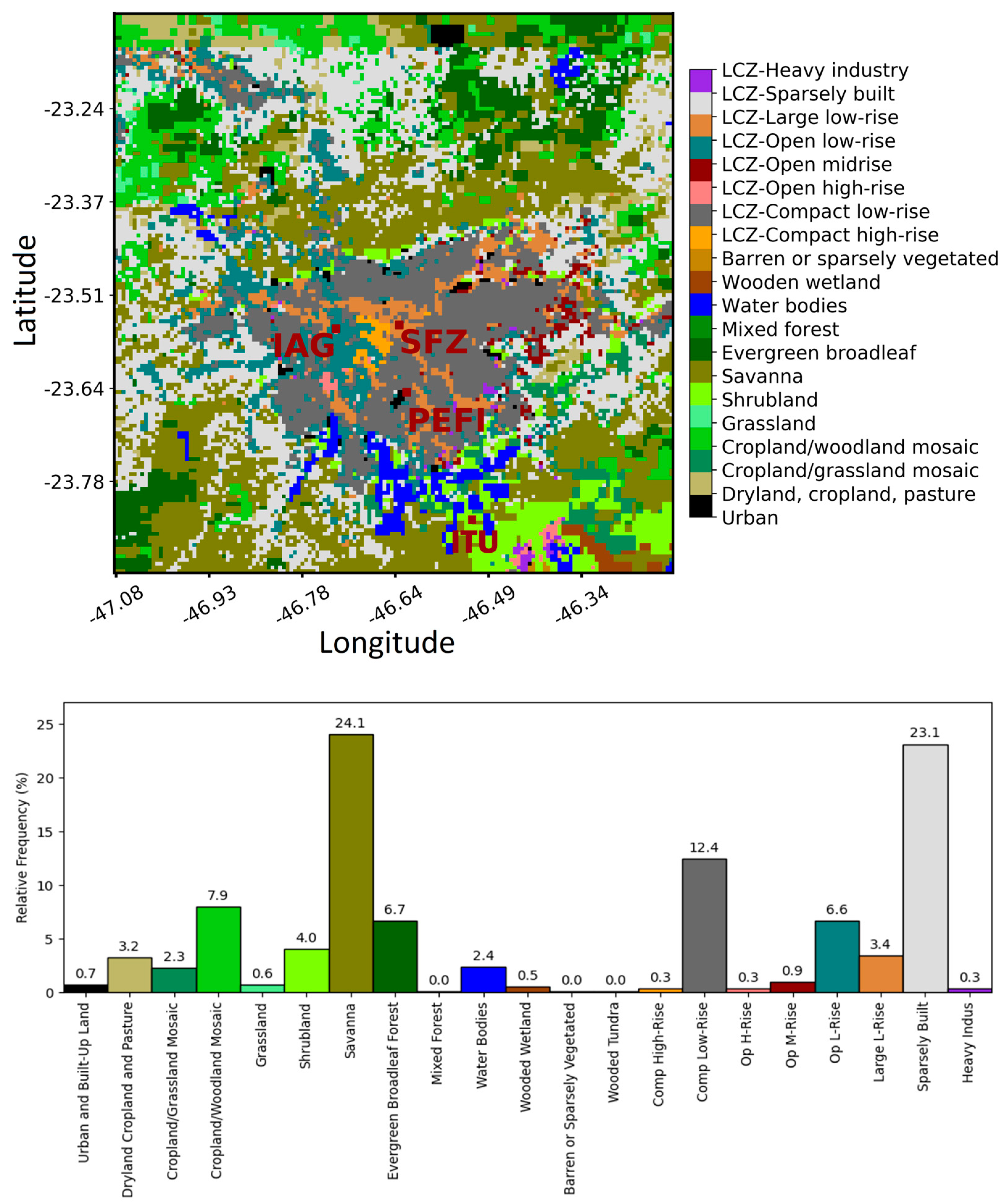
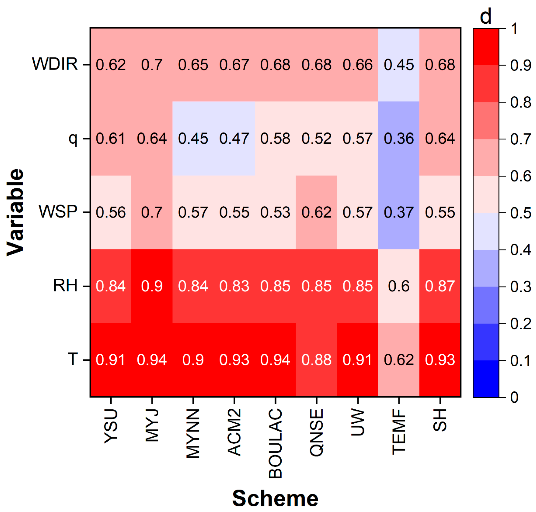
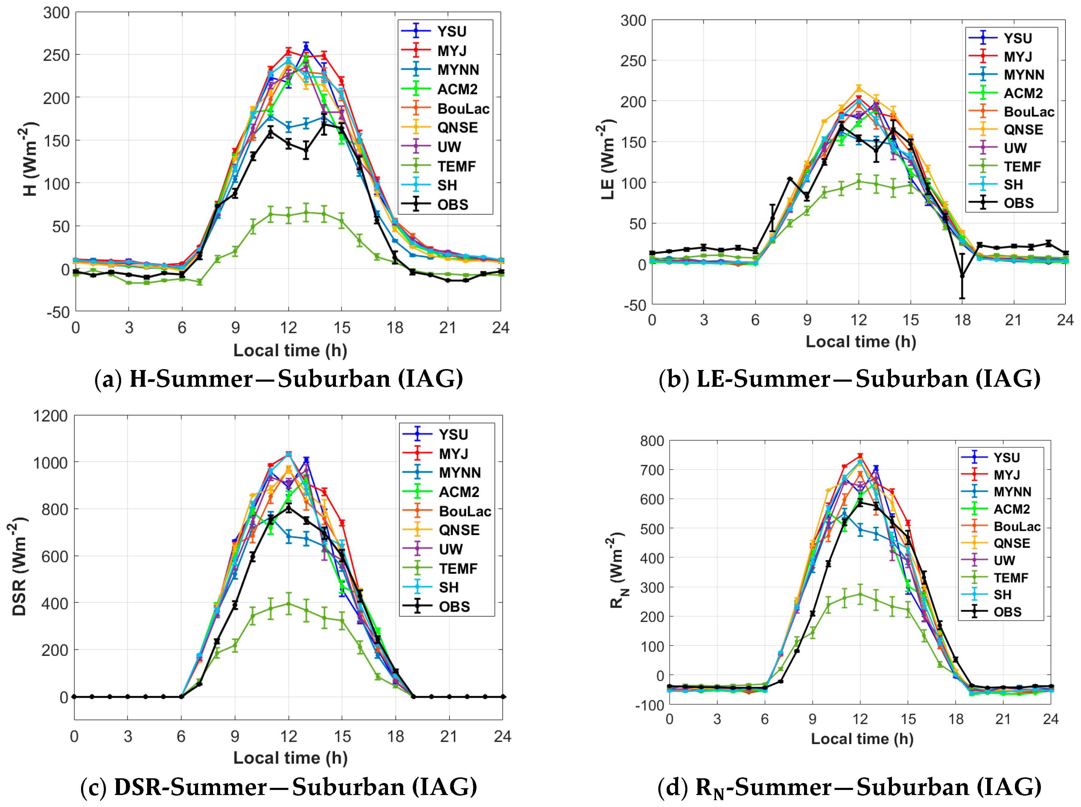

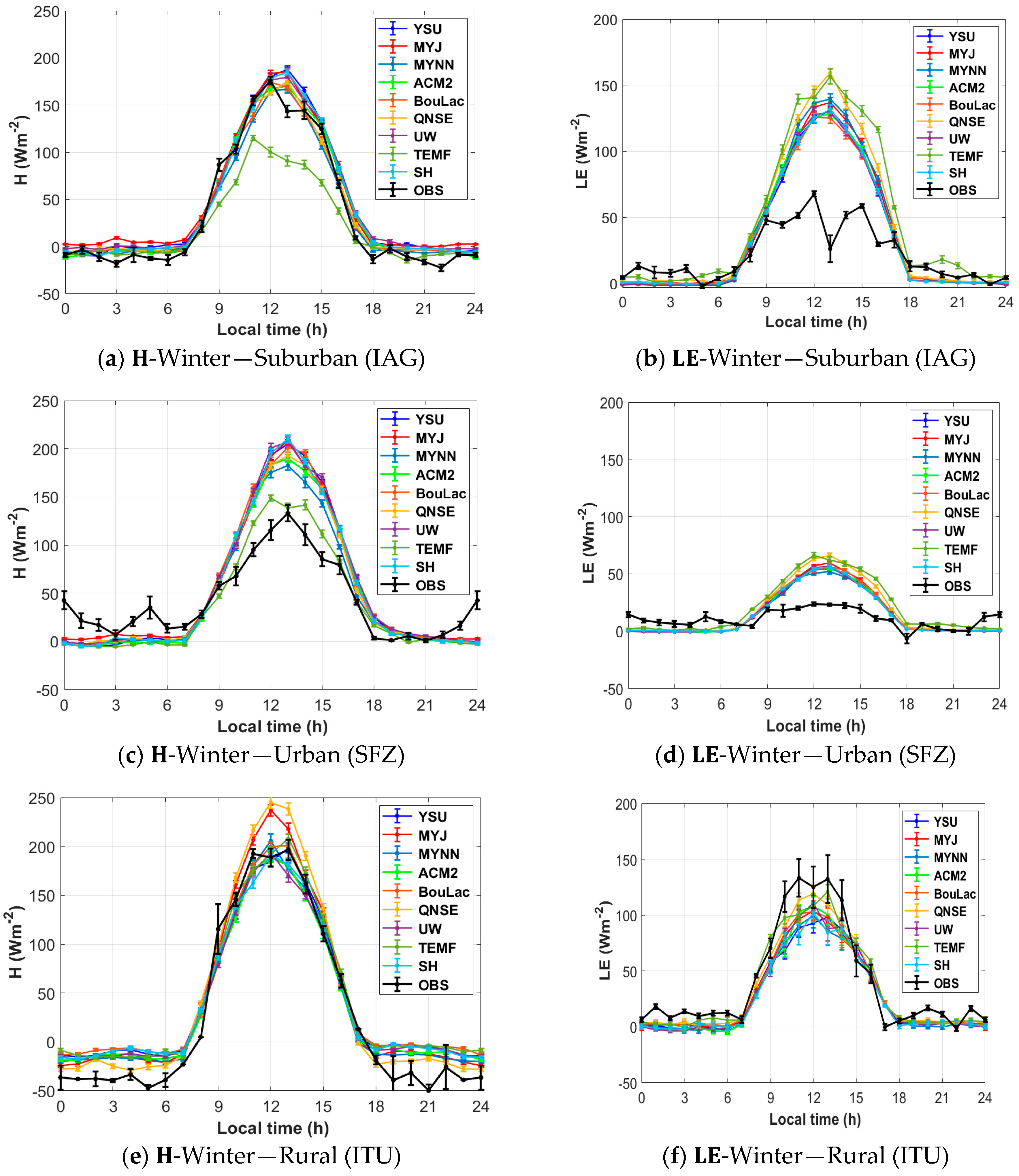
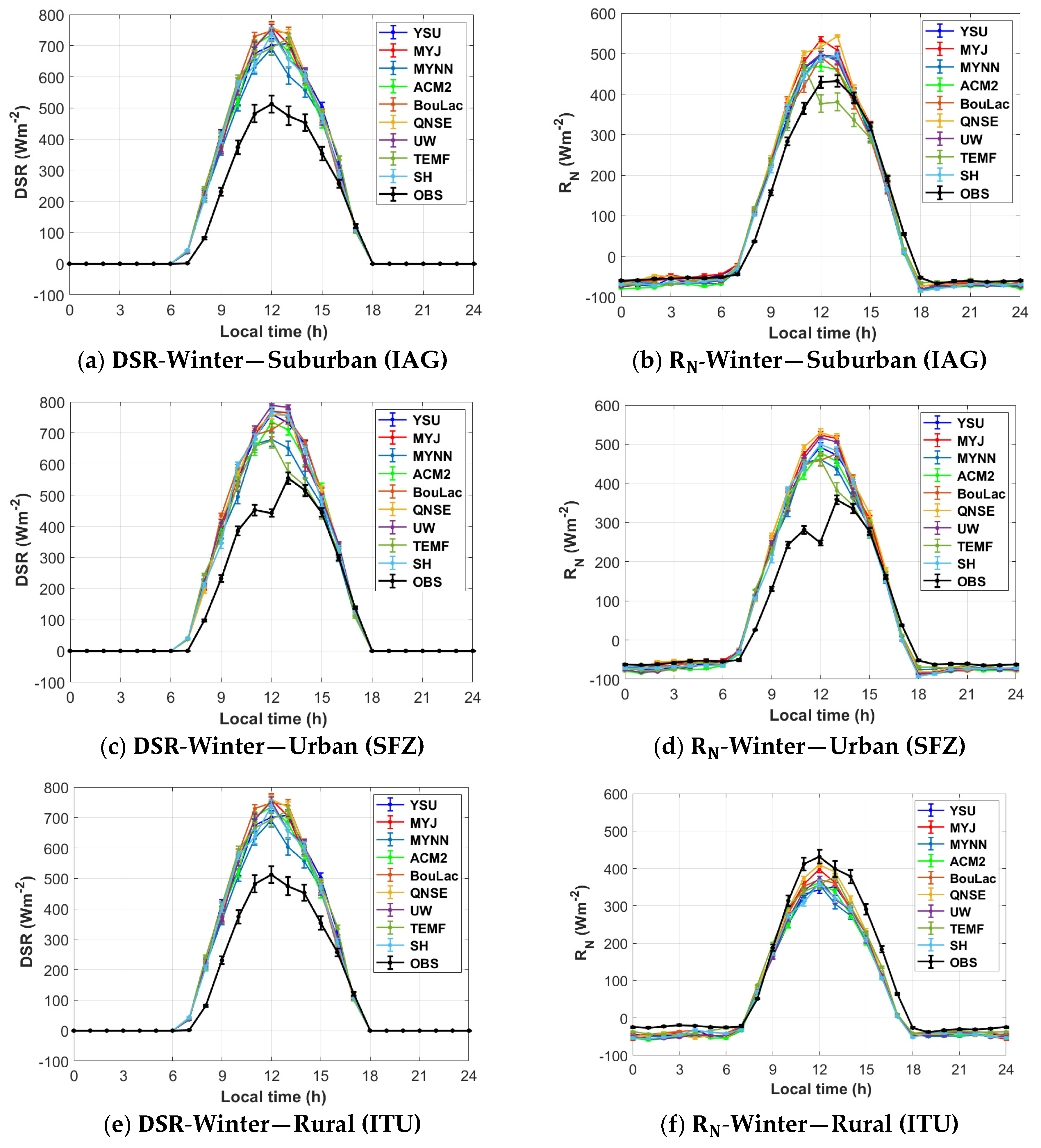
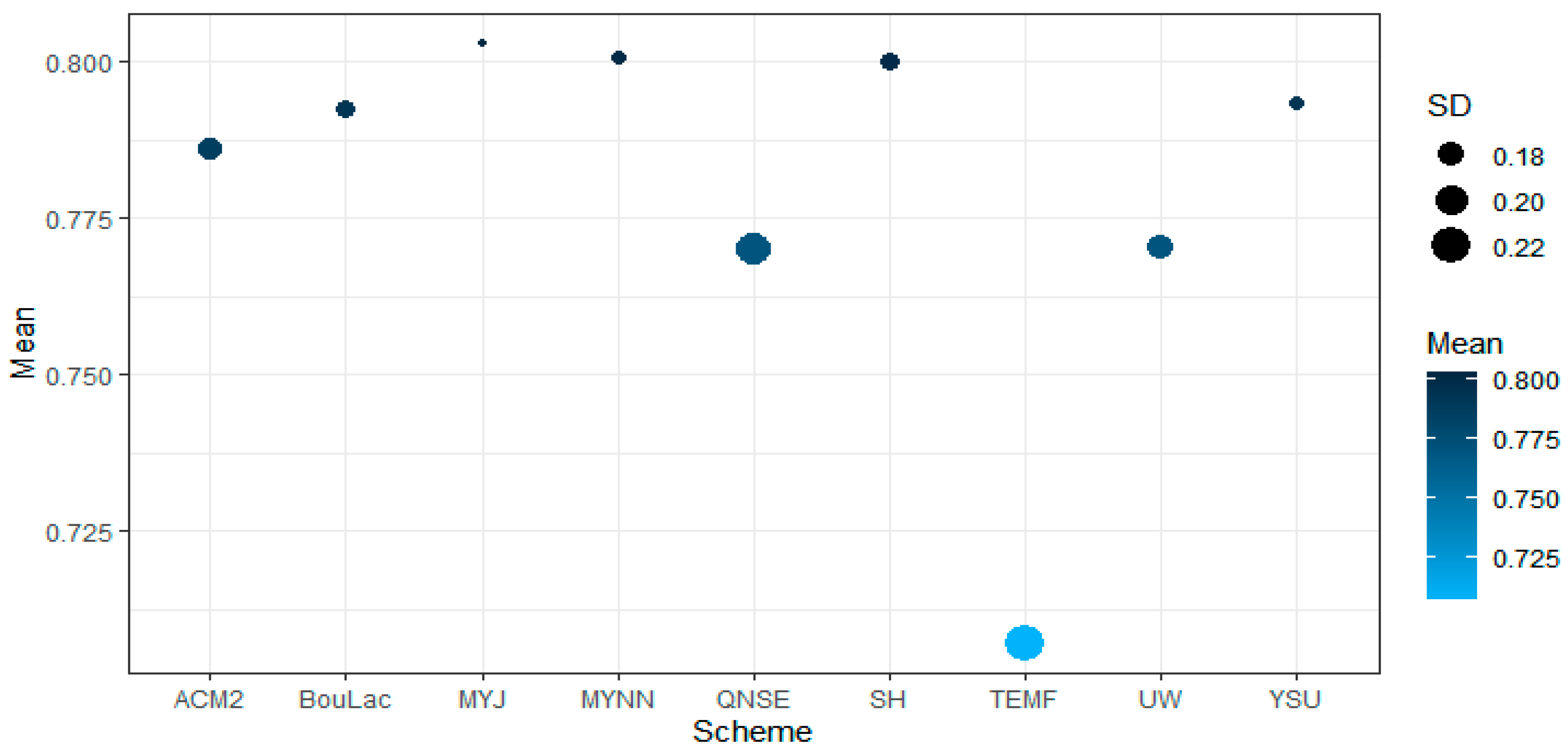
Disclaimer/Publisher’s Note: The statements, opinions and data contained in all publications are solely those of the individual author(s) and contributor(s) and not of MDPI and/or the editor(s). MDPI and/or the editor(s) disclaim responsibility for any injury to people or property resulting from any ideas, methods, instructions or products referred to in the content. |
© 2024 by the authors. Licensee MDPI, Basel, Switzerland. This article is an open access article distributed under the terms and conditions of the Creative Commons Attribution (CC BY) license (https://creativecommons.org/licenses/by/4.0/).