Abstract
Surface Water–Groundwater (SW–GW) interaction is a crucial aspect of the hydrological cycle and requires accurate modeling for reliable predictions. In many basic hydrological models and calculations, it is common to assume that the water density is constant. However, density-dependent flow, which accounts for changes in water density, plays a significant role in various hydrological processes. This study aims to quantify the effects of density-dependent flow on SW–GW interaction and evaluate the sensitivity of dominant hydrological drivers to density-dependent flow. Our simulations using the HydroGeoSphere model revealed that neglecting density-dependent flow in SW–GW interaction can lead to inaccurate estimations of water and solute balances. In particular, including density-dependent flow in the model yielded more realistic salinity distributions under gaining river scenarios and captured the gradual expansion of freshwater lenses under losing river scenarios. The results also indicated that under non-density-dependent flow, more saline groundwater is exposed to evapotranspiration, resulting in higher solute mass storage and a more saline unsaturated zone. Further, surface recharge and pumping rates played crucial roles in salinity distribution. This study highlights the critical importance of incorporating density-dependent flow in simulations, providing valuable insights for improving the accuracy of predictions and effectively managing water and solute balances in floodplain aquifers.
1. Introduction
Surface Water–Groundwater (SW–GW) interaction is a fundamental component of the hydrological cycle on the watershed scale. Surface water bodies (e.g., rivers, streams, lakes, and wetlands) continuously interact with the vadose zone and shallow and deep groundwater systems. Naturally, surface water and groundwater have different hydraulic dynamics and quality properties, meaning that one system’s quantity and quality could potentially affect the other [1]. Therefore, hydrological models must account for this interaction to provide reliable predictions [2,3]. The SW–GW interaction impacts a wide variety of functions, including biogeochemical cycling and habitats for diverse organisms [4,5,6], river ecology [7,8,9,10], as well as water, mass, and energy transfer at the catchment scale [11,12,13]. Furthermore, the SW–GW interaction plays a role in earth system modeling at continental and global scales [14,15].
In a hydrologically connected SW–GW system, the flow is determined by the disparity in hydraulic head between the surface water source and the underground water reservoir and the permeability of the partially porous sediment layers in the river. The majority of hydrogeological studies have primarily focused on the issue of groundwater flow by assuming a constant density of water and attributing the flow solely to pressure variations. This type of flow is commonly known as hydraulic-dependent flow [2,16,17]. This method is frequently employed for studying the behavior of fluid flow and solute dynamics. However, its reliability is limited to situations where there is no substantial difference in density between the two domains.
As temperature rises, fluid density decreases, while higher salinity increases fluid density [18]. Density-dependent (DD) flow, influenced by variations in water density [19], becomes dominant in significantly saline groundwater, leading to a mixed-convection formation [20]. This occurs when fluid flow is influenced by both forced and free convection, typical in scenarios where the non-uniform density distribution under gravity governs flow. The presence of density contrast complicates flow patterns and velocity fields in the aquifer [21,22], causing unstable density stratification due to dense saline water over less dense fresh groundwater [23].
DD flow is crucial in groundwater systems, potentially causing instabilities and accelerating solute spreading with substantial density contrast. The significance of DD flow and mass transport extends across various hydrogeological challenges, encompassing issues such as predicting the destiny of groundwater contaminants [24,25], understanding coastal hydrogeological processes [26,27,28], exploring geothermal resources [29,30,31], and addressing geological CO2 sequestration challenges [32,33,34]. A comprehensive understanding of this process is essential for accurate predictions and implementing effective measures to mitigate and prevent environmental issues.
The implication of DD flow is particularly noticeable when comparing a minor water density change to hydraulic head gradients. For instance, a subtle density variation of 1 kg/m3, only a 0.1% deviation from standard freshwater density (1000 kg/m3), can exert a comparable influence on water movement as a typical one-meter elevation change over a one-kilometer distance. Illustratively, a diluted seawater solution with approximately 2 g/L salinity, just 5% of regular seawater, showcases how even minor salinity variations are crucial for generating DD flow gradients. These gradients can rival the effects of the common hydraulic head gradients observed in natural settings [35]. Importantly, DD flow, governed by these subtle density differences, can either occur in isolation or in conjunction with flow driven by hydraulic forces, highlighting its versatility and significance in hydrological processes.
While there is growing interest in studying how density affects water flow, we have yet to fully understand these complex processes [36,37]. The system exhibits strong nonlinearity, where minimal changes in salinity directly influence density distribution, subsequently affecting pressure and influencing velocity distribution. The velocity field, governed by advection, drives solute concentration changes [38]. Eeman et al. [36] investigated freshwater lens thickness in the presence and absence of density contrast during recharge above saline water. Their analytical and numerical methods revealed substantial impacts on lens thickness due to the mass flux ratio and density difference, emphasizing the overestimation risk when ignoring density differences. Despite the recognized significance of DD flow as an exchange process, it has not been thoroughly investigated compared to hydraulic-dependent flow [39].
The interaction between saltwater and freshwater has been explained through two approaches, namely sharp interface and diffusive interface. The sharp interface assumes a small transition zone, immiscible fluids, and hydrostatic equilibrium [40,41], and is widely used for its simplicity [42,43,44,45]. However, recent research by Solórzano-Rivas et al. [46] has demonstrated its tendency to overestimate seawater intrusion and freshwater lens size. The diffusive interface, accounting for salt’s hydrodynamic dispersion [38], is more realistic. Fully coupled variable-density flow and advection–dispersion numerical models, empowered by enhanced computational capabilities and coupling techniques, represent a new era in solving differential equations for variably saturated subsurface flow and surface water flow (e.g., SEAWAT [47], HydroGeoSphere (HGS) [48], FEFLOW [49], SUTRA [50], OpenGeoSys [51]).
Interest has recently been increasing toward DD flow due to its importance in a range of ecological, environmental, and groundwater management issues. These include concerns with landfill sites [52,53], disposal basins and salt lakes [54,55], seawater intrusion [46,56], and salt accumulation in the unsaturated zone in arid/semi-arid areas [17,57,58]. Despite advancements in modeling DD flow, numerous ongoing studies, such as those examining leachate plumes from landfills or conducting tracer tests, still overlook DD flow effects. This is primarily due to the assumption, either implicitly or explicitly, that these effects are relatively small when compared to other processes involved in the study [35,38]. Alternatively, some studies employ the “equivalent freshwater head” approach as a step toward addressing this issue [59,60,61]. However, this approach can be overly simplistic or even erroneous, particularly when vertical flow is a focal point.
Over three decades, this has been an ongoing challenge to obtain a unique solution to accurately predict the quantity of fingers, their spatial distribution, sizes, migration rates, and pathways. For instance, the studies by Woods and Carey [62] and Van Reeuwijk, Mathias [63] confirmed the existence of multiple solutions to the classic elder problems. Highly unstable DD systems are so intricate that expecting a unique solution is seldom realistic. According to Xie et al. [64], a quantitative stochastic analysis of measurable macroscopic indicators such as the vertical center of mass, total solute mass, and Sherwood number (the ratio of the convective mass transfer to the rate of diffusive mass transport) provides a more reliable explanation for DD flow compared to a microscopic deterministic approach that considers factors like the number of fingers and the deepest plume front. Moreover, the injection of ionic or dye tracers, as employed by Harvey and Wagner [65], measures flow exchange between domains, but the known factors altering water density, resembling density-driven flow, are often not quantitatively evaluated [39].
Developing numerical models of DD hydrogeologic systems is complex and involves high uncertainty. Therefore, simplification seems necessary, but the extent of acceptable simplification and the implications are not always clear. It is unclear how important each process is and under what conditions they can safely be ignored [35]. While DD flow is indispensable in certain cases, such as seawater intrusion and the analyses of salt lakes and landfills, constraints related to process time and resources limit the spatial scale and resolution for accurate simulations [66]. In certain situations, simplifying the analysis by excluding DD flow may be feasible. Such conditions could include scenarios where the salinity contrast is negligible, or where the hydraulic gradient is substantial. Situations with high rates of recharge, pumping, or evapotranspiration also qualify, as do cases considering the influence of river dimensions on SW–GW interactions, large-scale hydrogeological studies, or those involving periodic anthropogenic variables. However, the full implications of this simplification in these contexts remain uncertain and require cautious consideration.
This research aims to investigate the impact of DD flow on SW–GW interactions, determining when simulations should consider DD flow or when simplified analyses suffice. The study seeks insights into the extent of DD flow’s influence on the SW–GW interaction process, focusing on two main objectives as follows: quantifying DD flow effects on SW–GW interactions and assessing the sensitivity of dominant hydrological drivers to DD flow. To achieve these goals, various scenarios have been designed to evaluate whether incorporating DD flow simulations significantly enhances result accuracy. All scenarios will undergo simulations with and without DD mode, ensuring a comprehensive evaluation of its influence.
2. Materials and Methods
2.1. Conceptual Model and Scenarios
In this study, our aim was to gain insights into the intricate hydrological processes within a coastal floodplain environment, specifically focusing on understanding the impacts of density-dependent flow on the interactions between surface water (SW) and groundwater (GW) in a riparian setup. To achieve this, we employed a conceptual model designed to capture the complexities of the system. This model accounts for key factors including river–floodplain flow regimes, evapotranspiration (ET), surface recharge from rainfall, groundwater pumping, and the salinity contrast (Total Dissolved Solids—TDS) between SW and GW. Our conceptual model is presented as an idealized cross-section perpendicular to a river and an aquifer, as illustrated in Figure 1. The dimensions of the domain are 20 m, 0.1 m, and 5 m in the x, y, and z directions, respectively. The river is represented in a rectangular shape with a depth of 1.5 m and a width of 2 m. The investigated hydrological drivers are outlined in Table 1.
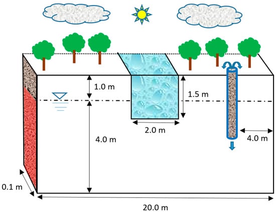
Figure 1.
The conceptual model of the study case. Fresh surface water and saline groundwater boundaries are shown in blue and red, respectively. Note that the figure is not drawn to scale.

Table 1.
Defined scenarios for each investigated driver.
To investigate the impact of DD flow under varying hydrological conditions, two distinct scenarios were defined as follows: the gaining river scenario and the losing river scenario. This approach aims to assess how DD flow influences rivers when they experience different flow dynamics. In the gaining river scenario, the focus is on situations where the input of water, including DD flow, exceeds losses due to factors like evaporation and outflow. Conversely, the losing river scenario explores conditions where water losses surpass the incoming flows, resulting in diminished river discharge. By analyzing these contrasting scenarios, a comprehensive understanding of the implications of DD flow on river systems can be gained under diverse hydrological circumstances.
Table 1 outlines the specific scenarios under investigation, each designed to reflect the various impacts of these drivers. We employed both DD and NDD flows in our simulations, resulting in a comprehensive set of seven different scenarios. All simulations were conducted under steady-state unsaturated flow conditions over a five-year period, maintaining constant boundary condition values. Given the theoretical nature of this exploration, we did not subject them a calibration process. Instead, our emphasis was on elucidating the relative impacts of DD flow on water and solute balances within the floodplain aquifer.
2.2. Numerical Model
Given the complexity of the hydrological processes and the need for reliable and stable numerical methods, the research chose to utilize the HydroGeoSphere (HGS) model developed by Therrien et al. [48]. HGS is a three-dimensional numerical model that effectively captures and integrates the dynamics of surface and subsurface flow as well as solute transport. It employs a modified version of Richards’ equation to describe the three-dimensional transient subsurface flow in a variably saturated porous medium. Two relationships, namely van Genuchten [67] and Brooks–Corey [68], were utilized to calculate the pressure–saturation relationship and relative hydraulic conductivity. The simulation of surface flow is achieved by employing a two-dimensional depth-averaged flow equation, which is a diffusion–wave approximation of the Saint Venant equation. The HGS model offers the following two approaches for coupling surface and subsurface processes: the common node approach, which ensures hydraulic head continuity between the two domains, and the dual node approach, which incorporates a first-order exchange coefficient. Here, the dual node approach was employed. Vegetation transpiration takes place within the subsurface’s root zone, influenced by factors such as leaf area index (LAI), nodal water content, and root distribution function (RDF) within a specified extinction depth. On the other hand, evaporation from both the soil surface and subsurface soil layers is determined by the nodal water content and an evaporation distribution function (EDF) across a prescribed extinction depth. The detailed mechanisms of three-dimensional solute transport in a variably saturated porous matrix have been further elaborated by Therrien et al. [48].
In this particular study, the HGS model employed the control volume difference element approach. The initial time step was set to 0.1 days, and a maximum time step of 10 days was used. To solve the non-linear equations for the variably saturated subsurface flow, surface flow, and solute transport, the model utilized the Newton–Raphson linearization method. Several parameters were specified for the Newton iteration process, including a maximum of 25 iterations, a Jacobian epsilon of 10.0 d−5, an absolute convergence criterion of 1.0 d−5, and a residual convergence criterion of 1.0 d−3. The flow solver had a maximum iteration limit of 1.0 d–5. Additionally, the Groundwater Modeling System (GMS) developed by Aquaveo [69] was employed as a postprocessor. The Groundwater Modelling System (GMS) was used to visualize and interpret the model outputs obtained from HGS.
2.3. Geometry Grid
The dimensions, boundary conditions, groundwater flow, and salinity dynamics were assumed to be symmetrical. Therefore, as shown in Figure 2, the geometry grid covers the left side of the conceptual model. A partially penetrating stream was constructed on the upper right side of the grid with 1.5 depth and 1 m width. The aquifer was considered an isotropic homogenous porous media to exclude the effect of heterogeneity and focus on the role of DD flow. The water table was located at 4 m, creating a 1 m deep unsaturated zone in the porous media and 0.5 m water depth in the river. It was discretized into 0.2 m * 0.1 m * 0.2 m grids in x, y, and z directions to balance the required computational time and efficient spatial representation of the domain. The final geometry grid consisted of 2652 nodes that formed 1250 elements.
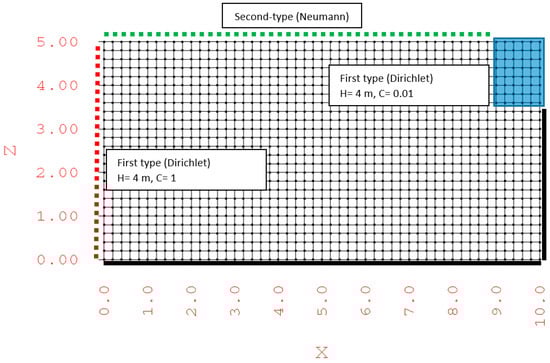
Figure 2.
The geometry grid and boundary conditions of the study case (H = head and C = concentration). No-flow boundary condition is shown with solid black lines.
2.4. Boundary Conditions
Two types of boundary conditions were implemented in the model as follows: first-type (Dirichlet) boundaries, where the head or concentration values are prescribed, and second-type (Neumann) boundaries, where the flow or solute flux values are prescribed. In the subsurface domain, a first-type (Dirichlet) boundary condition was applied at the left side of the domain, where a constant head of 4 m was specified. This boundary condition is depicted in Figure 2. Similarly, the river, 4 m constant head, was imposed using the first-type (Dirichlet) boundary condition at the top right of the domain. The first-type (Dirichlet) concentration boundary condition was used to represent the salinity boundary conditions. Thus, a constant value of 1 was assigned to the left outer boundary and 0.01 to the river nodes to characterize the saline groundwater and fresh river water, respectively (Figure 2). The recharge (rainfall) was modeled for the entire model surface domain using second-type (Neumann) boundary conditions for the defined scenarios. The ET (Evapotranspiration) scenarios in the model were dynamically simulated by considering a combination of evaporation and transpiration processes. This was achieved by extracting water from all the model cells within the specified zone of evaporation and root extinction depths in both the surface and subsurface flow domains. Moreover, water and solute were extracted or added as 1D free-surface flow and solute transport through the nodes along the axis of the well. Details of the types of boundary conditions and the governing equations can be found in the HGS user manual by Therrien et al. [48].
The initial condition for the scenario simulations was obtained from a long-term steady-state model run, which was carried out for a duration of 20,000 days to achieve equilibrium conditions. In this initial model, no hydraulic gradient was imposed (both surface water and groundwater were at a head of 4 m), and it did not consider factors such as evapotranspiration (ET), recharge, or pumping. Figure 3 illustrates the initial condition models for both DD and NDD flow, which were used as the initial conditions for all subsequent scenarios.
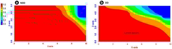
Figure 3.
Initial condition models for NDD and DD. Elements edges are shown with black lines.
2.5. Parametrization
The subsurface domain was considered as homogenous porous media with sand soil. The soil properties of the model and unsaturated van Genuchten function parameters [67] were adopted from Carsel and Parrish [70]. The surface flow domain properties were adopted from Doble et al. [71]. A function was applied to the surface domain for the ET scenarios to represent grass with values from Alaghm et al. [2]. Table 2 summarizes all the parameters’ values used in this study.
Table 2.
Parameter values of the model for the numerical model.
3. Results and Discussion
3.1. Initial Condition Model
Upon examining the initial conditions, it was observed that NDD resulted in an overestimation of the stored solute mass within the domain relative to the DD model, with values of 1.68 kg and 1.59 kg for NDD and DD (≈5.50%), respectively. Additionally, the NDD model generated a more saline unsaturated zone (z > 4 m) compared to the DD model, consequently underestimating the extent of the freshwater lens. Figure 4 represents the distribution of solute mass in both the unsaturated and saturated zones.
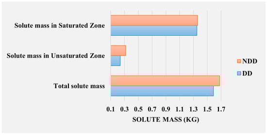
Figure 4.
Simulated stored solute mass for both NDD and DD.
The discrepancies observed between the NDD and DD models can be attributed to the influence of DD flow on the SW–GW interactions. DD flow accounts for the variation in fluid density due to solute concentration, which, in turn, affects the flow dynamics and solute transport processes. Neglecting this DD behavior in the NDD model can lead to significant deviations in the predicted system response. The current findings align with previous research and emphasize the need to consider DD flow processes in SW–GW interaction models. Several studies have highlighted the importance of incorporating DD flow mechanisms in hydrological modeling. For instance, Panday et al. [72] demonstrated that neglecting the DD effects in groundwater models can result in inaccurate predictions of solute transport and contaminant plume evolution. In another study by Torres Martínez et al. [73], it was found that the inclusion of DD flow improved the accuracy of simulated groundwater levels and salinity profiles in coastal aquifers. By accurately representing the effects of solute concentration on fluid density, these models can provide more reliable predictions of solute transport, salinity distribution, and the overall behavior of the subsurface system.
3.2. River–Floodplain Flow Regime
In hydraulically connected river–floodplain systems, the hydraulic gradient plays a crucial role in controlling the interaction between SW and GW domains. To examine the influence of DD flow under different flow conditions, two scenarios were defined, namely gaining river and losing river.
3.2.1. Gaining River
A river is considered gaining when the higher hydraulic gradient is in the floodplain aquifer, resulting in flow towards the river. In this scenario, the aquifer recharges the adjacent river through the riverbank or bed. Figure 5 and Figure 6 illustrate the gaining river scenarios under both DD and NDD, with various hydraulic gradients towards the river.
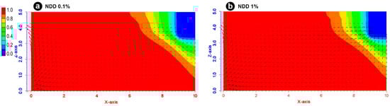
Figure 5.
NDD salinity distribution for gaining river with 0.1% and 1% hydraulic gradients. Darcy velocity vectors are shown with black arrows where the length is scaled by its magnitude.
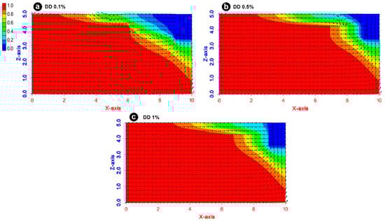
Figure 6.
DD salinity distribution for gaining river with (a) 0.1% hydraulic gradients, (b) 0.5% hydraulic gradients, and (c) 1% hydraulic gradients. Darcy velocity vectors are shown with black arrows.
Figure 5 shows that under NDD, increasing the hydraulic gradient towards the river from 0.1% to 1% does not significantly impact the salinity distribution. However, recharge towards the river increases proportionally with the increase in hydraulic gradient, as indicated by the Darcy velocity vectors.
Under DD flow (Figure 6), as the hydraulic gradient increases, the floodplain aquifer evolves into a more saline system. Despite both density and hydraulic forces acting towards the river, at low hydraulic gradients (0.1% and 0.5%), the freshwater lens sustains to some extent. This can be attributed to the buoyancy effect that occurs in saline aquifers adjacent to gaining rivers. Werner and Laattoe [74] discussed this phenomenon and concluded that the river may simultaneously lose freshwater and gain saltwater. This behavior is reflected in Figure 6a,b, where mixed convection is observed at specific locations (x = 5–9 and x = 7.4–9) for hydraulic gradients of 0.1% and 0.5%, respectively. However, when the gradient becomes too high (1%), free convection dominates, and the freshwater lens associated with the gaining river disappears (Figure 6c).
3.2.2. Losing River
The simulations for losing river scenarios are presented in Figure 7, where the head at the left side of the domain gradually decreases, representing the hydraulic gradient towards the groundwater aquifer in a losing river.
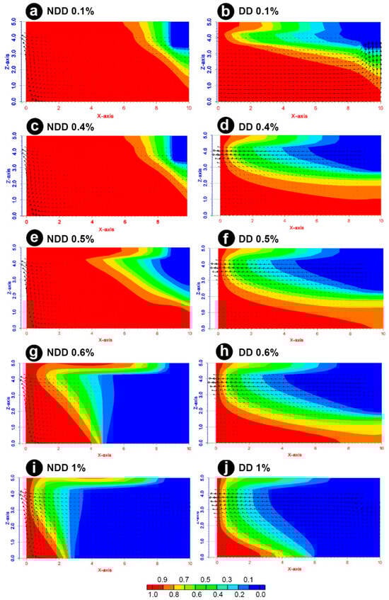
Figure 7.
NDD and DD salinity distribution for losing river with different hydraulic gradients (a–j). Darcy velocity vectors are shown with black arrows where the length is scaled by its magnitude.
Under NDD, the solute dynamics significantly differ between the low and high hydraulic gradients. When the gradient is less than or equal to 0.5%, NDD overestimates the solute mass in low hydraulic gradients compared to DD (Figure 7a,c,e). However, when the gradient exceeds 0.5%, NDD exhibits an underestimation of solute mass (Figure 7g,i). In contrast, DD captures a more realistic gradual expansion of the freshwater lens, where the size of the lens increases proportionally with the increase in hydraulic gradient from 0.1% to 1% (Figure 7b,d,f,h,j). The different patterns observed in the dynamics of the freshwater lens for NDD and DD are shown in Figure 8. As depicted in Figure 8, it is evident that the salinity dynamics under DD are highly sensitive to changes in the hydraulic gradient. However, it is important to note that NDD requires a hydraulic gradient of at least 0.5% to observe the initial change in salinity distribution.
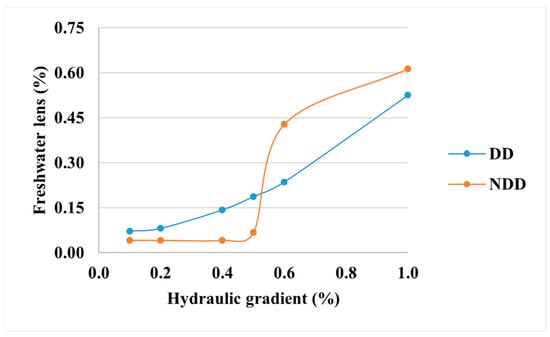
Figure 8.
Simulated freshwater lens size (% of total domain) for the defined scenarios.
At very low hydraulic gradients under DD (0.1%), the groundwater aquifer recharges the river through the riverbed, which may seem counterintuitive for a losing river (Figure 7b). This phenomenon indicates that at no or very low hydraulic gradients, forced convection governs the solute dynamics rather than free convection. This behavior is reflected in Figure 9a, which demonstrates the net flux (influx–outflux) at each time-step for the losing river scenarios. Despite the hydraulic gradient away from the river, when the gradient is low (0.1% and 0.2%), the net flux is negative (aquifer recharges river). As the gradient increases, the net flux becomes positive (river recharges aquifer). In contrast, NDD does not exhibit this dynamic and always shows a balance in flux exchange between the river and the aquifer.
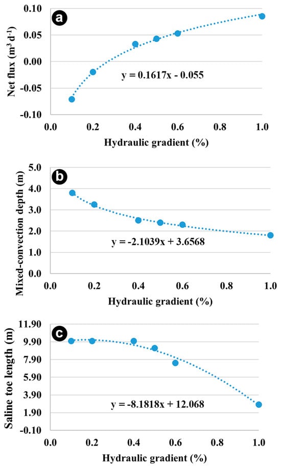
Figure 9.
Net flux exchange (Influx–Outflux) (a), Mixed-convection depth (b) and saline toe length (c) for the losing river scenarios under DD.
DD effectively captures the process of fresh water (lighter) overlying saline water (heavier), resulting in mixed convection. For example, mixed convection can be observed at z = 2.6 m with a 0.4% gradient, compared to z = 1.8 m under a 1% gradient (Figure 9b). Moreover, mixed convection results in a longer saline toe under DD compared to NDD, where the toe is only attributed to free convection. For instance, the saline toe is 2.8 m for DD and 2 m for NDD under a 1% hydraulic gradient, as shown in Figure 7i,j, respectively. Overall, it appears that the larger the hydraulic gradient away from the river, the shorter the saline toe, as reflected in Figure 9c.
The findings from the gaining and losing river scenarios highlight the importance of considering DD flow in river–floodplain systems. DD flow plays a crucial role in controlling salinity distribution, the behavior of the freshwater lens, and the dynamics of solute transport. The observations from this study are consistent with previous research that emphasizes the significance of DD flow in riverine systems. For example, Yabusaki et al. [75] discussed the complex behavior of salinity dynamics in river–floodplain systems and highlighted the interplay between density and hydraulic forces. Their findings support the results obtained in this study, emphasizing the importance of considering DD processes for accurate modeling of river–floodplain interactions.
3.3. ET
In arid and semi-arid regions characterized by shallow groundwater tables, evapotranspiration (ET) plays a crucial role in soil salinization. To investigate the implications of DD on the ET process in a shallow floodplain aquifer, a group of scenarios was defined in this study. As discussed in Section 3.1, the unsaturated zone under NDD flow was more saline compared to DD. Therefore, under NDD, more saline groundwater was exposed to ET, as indicated by the root depth (0.2 m) and evaporation depth (1 m) considered in the simulations. As expected, higher ET rates resulted in a higher amount of stored solute mass in the domain and a more saline unsaturated zone. Both models (NDD and DD) show a similar pattern of overall increase in solute mass in the porous media due to constant ET over the five-year study period (Figure 10).
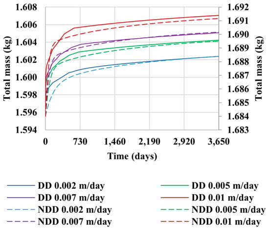
Figure 10.
Total solute mass stored in the porous media for NDD and DD models with different ET rates. The left-side vertical axis is for the DD model, and the right-side vertical axis is for the NDD model.
The impact of ET on solute transport and salinity distribution should be carefully considered in the management and planning of water resources in arid and semi-arid regions, as excessive ET rates can exacerbate soil salinization and negatively affect agricultural productivity and ecosystem health. Several studies have investigated the role of ET in soil salinization processes and its interaction with groundwater dynamics. For example, Alaghm et al. [16] examined the impact of groundwater declines and increased ET rates on the mobilization and transport of salinity in semi-arid regions. Their findings emphasized the importance of considering ET processes when assessing the vulnerability of groundwater systems to salinization. Similarly, Liu et al. [76] investigated the influence of ET on salt accumulation in soils in arid regions, highlighting the need for accurate modeling of ET processes to effectively manage salinity issues. These findings underscore the significant role of ET in soil salinization processes, particularly in arid and semi-arid regions with shallow groundwater tables.
3.4. Recharge
Recharge is a fundamental process through which groundwater aquifers receive freshwater, and it also affects the transport of solute mass within the aquifer. Recharge can occur through influx from the riverbank in losing river scenarios (as discussed in Section 3.2.2) or as surface recharge from rainfall. The impact of recharge on groundwater salinity dynamics under both NDD and DD simulations is illustrated in Figure 11.
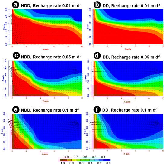
Figure 11.
Simulated salinity distribution for the defined recharge rates (a–f). Darcy velocity vectors are shown with black arrows where the length is scaled by its magnitude.
The results reveal that salinity dynamics are highly sensitive to surface recharge rates in both NDD and DD simulations. When a small recharge rate of 0.01 m/day is applied (Figure 11a,b), a freshwater lens forms under NDD, and the existing freshwater lens expands under DD. Furthermore, for low recharge rates under NDD, the freshwater lens is underestimated compared to DD. However, as the recharge rate gradually increases, the freshwater lens becomes overestimated under NDD compared to DD flow. This is reflected in Figure 12a, which demonstrates the stored solute mass for both NDD and DD. As the recharge rate increases, the groundwater aquifer gradually becomes less saline. The pattern is slightly different for the unsaturated zone, as shown in Figure 12b. There is a dramatic decrease in solute mass in the unsaturated zone at low recharge rates up to 0.03 m/day, after which it becomes stable. This indicates that a limited amount of solute mass stored in the unsaturated zone is washed off at the beginning of the recharge process, and after a certain point, there is no significant amount of solute mass remaining in the unsaturated zone.
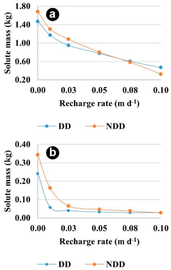
Figure 12.
(a) Total simulated stored solute mass for both NDD and DD. (b) Simulated stored solute mass for both NDD and DD in the unsaturated zone.
Figure 12 depicts the different water balance dynamic patterns for NDD and DD under the defined recharge rates. Additionally, Figure 13 illustrates the simulated net flux (influx–outflux) via the river and groundwater boundary conditions (first-type, Dirichlet). When simulating under NDD, the net flux is continuously negative (outflux > influx) and changes linearly with increasing recharge rate. However, the application of surface recharge under DD generates a significantly different pattern due to the buoyancy effect. At lower recharge rates, below 0.02 m/day (Figure 12b), forced convection dominates, and a relatively small, recharged flow floats over the denser, heavier saline groundwater, pushing it slightly downward and allowing more influx from the river into the aquifer. However, the net flux remains negative. When the recharge rate becomes large enough, greater than 0.05 m/day, free convection takes over, pushing the denser saline groundwater further down. This results in more freshwater influx from the river, leading to a positive net flux.
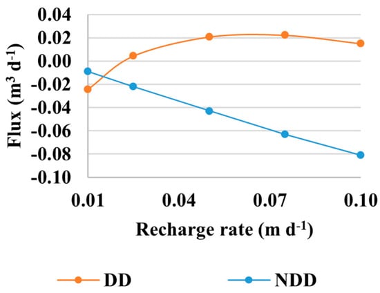
Figure 13.
Simulated net flux under the defined recharge rates for both NDD and DD.
The findings emphasize the significance of recharge rates in influencing groundwater salinity dynamics and the exchange of water between the river and the aquifer. The behavior of the net flux, particularly under DD, highlights the complex interplay between DD flow and the recharge processes. These findings have important implications for water resource management and salinity control strategies in river–floodplain systems, as accurate estimation of recharge rates is crucial for understanding the movement of solute mass and freshwater distribution within the aquifer.
Several studies have investigated the influence of recharge on groundwater salinity dynamics and the interaction between surface water and groundwater systems. For instance, Moeck et al. [77] conducted a global assessment of groundwater recharge rates and emphasized the importance of accurate recharge estimation for sustainable groundwater management. Additionally, Scanlon et al. [78] investigated the impact of recharge variability on groundwater salinization in semi-arid regions, highlighting the role of climate variability and recharge processes in controlling groundwater salinity. Furthermore, the influence of recharge on solute transport and salinity dynamics in river–floodplain systems has been studied by various researchers. For example, Zhang et al. [79] examined the impact of recharge on solute transport in river–floodplain environments and highlighted the importance of considering recharge processes in modeling studies. Similarly, Costall et al. [80] investigated the effects of recharge variability on saltwater intrusion in coastal aquifers, emphasizing the need for accurate representation of recharge rates in numerical models. These studies, along with the findings of the current study, contribute to our understanding of the complex interplay among recharge, DD flow, and groundwater salinity dynamics in river–floodplain systems. They underscore the importance of considering recharge rates and their spatial and temporal variability when assessing and managing groundwater resources in arid and semi-arid regions with shallow groundwater tables.
3.5. Pumping
Pumping is a primary method of groundwater extraction and plays a crucial role in influencing the interaction between the SW and GW domains. Pumping can potentially alter the flow exchange between a river and the adjacent aquifer, consequently impacting the salinity dynamics of the groundwater aquifer. The simulated pumping scenarios are illustrated in Figure 14.
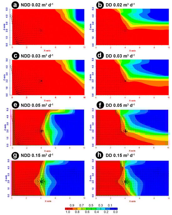
Figure 14.
Simulated models for pumping scenarios (a–h). Darcy velocity vectors are shown with black arrows where the length is scaled by its magnitude.
Under DD modeling approaches, the salinity dynamics are highly responsive to pumping, even at low rates. In contrast, under NDD modeling approaches, the salinity distribution responds to relatively higher pumping rates, typically larger or equal to 0.05 m3/day. This is evident in Figure 14a,c,e. As soon as the salinity distribution starts to be influenced by pumping, the NDD model overestimates the extent of the freshwater lens compared to DD for the same pumping rate, as demonstrated in Figure 14e,f,g,h. This contrasting behavior of the NDD model is observed not only under pumping scenarios but also under losing river (Section 3.2.2) and recharge (Section 3.4) scenarios.
The size of the freshwater lens proportionally increases as the pumping rate increases. Under DD, the expansion of the freshwater lens initially occurs horizontally. However, when the edge of the freshwater lens reaches the location axis of the pump (x = 5 m), it continues to grow vertically. This demonstrates the significant impact of the pump’s location on the salinity dynamics of the aquifer.
Simulations conducted under NDD and DD for relatively low pumping rates (less than 0.1 m3/day) generate significantly different results in terms of both flow patterns and salinity distributions. However, at high pumping rates, the outcomes become similar. This can be observed in Figure 14g,h, which show that at high pumping rates, pumping becomes the dominant factor shaping the salinity distribution and flow pattern, overriding the influence of free and forced convections.
The findings of this study highlight the importance of considering pumping rates and their effects on the salinity dynamics and flow patterns in river–aquifer systems. Pumping-induced changes in the groundwater salinity distribution have implications for water supply and management, particularly in regions where salinization poses a significant challenge. The impact of pumping on groundwater salinity dynamics and the interaction between surface water and groundwater systems has been extensively investigated in previous studies. Peters et al. [81] conducted a study on the impact of pumping on groundwater salinization in coastal aquifers and emphasized the need for sustainable pumping practices to prevent saltwater intrusion. Further, the influence of pumping on flow patterns and solute transport in river–aquifer systems has been studied by various researchers. Zhu et al. [82] examined the impact of pumping on flow patterns and contaminant transport in a riverbank filtration system and emphasized the need for integrated management strategies to optimize water supply and quality. These findings underscore the need for sustainable pumping practices and integrated management approaches that consider the spatial and temporal variability of pumping rates in order to mitigate salinization risks and ensure the long-term sustainability of groundwater resources.
3.6. SW–GW Density Contrast
In a porous medium with a non-uniform density distribution, the flow behavior can be characterized as mixed convection, which is a combination of forced convection driven by DD processes, and free convection, which is driven by hydraulic gradients. In a hydraulically connected SW–GW system with a fixed gradient, the flow pattern and salinity distribution undergo changes as the salinity contrast between the SW and GW increases. The simulated salinity distributions for various salinity contrast ratio scenarios are illustrated in Figure 15.
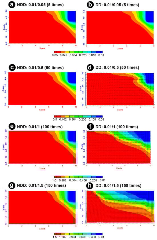
Figure 15.
Simulated models for the salinity contrast scenarios (a–h). Darcy velocity vectors are shown with black arrows.
When the salinity contrast is low, with the GW being less than 50 times more saline than the SW, free convection dominates the flow behavior. As a result, the DD and NDD flow simulations exhibit similar patterns, as shown in Figure 15a,b. However, as the salinity contrast increases to around 50 times, the influence of forced convection becomes apparent, leading to a slightly larger freshwater lens. This impact becomes more significant when the GW is 100 times or more saline than the SW. Overall, these findings demonstrate that larger freshwater lenses occur when there is a higher density contrast between freshwater and saltwater. Moreover, an increase in the salinity contrast results in the expansion of the mixed convection zone, both horizontally and vertically, as highlighted in Figure 15d,f,h.
The findings of the current study highlight the importance of considering the density contrast between SW and GW in understanding and managing SW–GW interactions. The density contrast not only affects the flow patterns and salinity distribution but also plays a crucial role in the transport of solutes and contaminants in SW–GW systems.
4. Limitations, Implications, and Future Work
Despite the valuable insights gained from our study, it is essential to acknowledge the inherent limitations. The HydroGeoSphere (HGS) model relies on specific parameterizations and simplifications, potentially introducing uncertainties related to geological variability and aquifer heterogeneity. Our steady-state approach, while informative, may not fully capture the dynamic nature of riparian systems. Future research should explore advanced modeling approaches that consider temporal variability and address the complexities associated with different geological conditions, enhancing the robustness of predictions.
The implications of our work carry significant weight for real-world applications, particularly in the realms of water resource management and environmental planning. Our study, which delves into the intricate dynamics of DD flow on SW–GW interactions, provides actionable insights that can directly inform decision-making processes. Regions grappling with salinity issues, such as coastal areas and arid regions, stand to benefit from the nuanced understanding we have gained. By incorporating the impact of DD processes, resource managers and policymakers can make more accurate predictions regarding salinity distribution, groundwater dynamics, and solute transport in river–floodplain systems. This newfound knowledge holds practical relevance for mitigating salinization risks, optimizing water supply, and maintaining the long-term sustainability of groundwater resources. Furthermore, our study paves the way for the development of decision-support systems that integrate DD considerations, ensuring that real-world strategies are grounded in robust scientific understanding.
The implications extend beyond the immediate scope of our study, offering a valuable foundation for addressing salinity challenges in diverse hydrogeological settings and providing a basis for adaptive strategies in the face of changing climate conditions. Future research endeavors could focus on integrating our results into decision-support systems for real-world applications. Exploring the impacts of climate change on SW–GW interactions, extending the applicability of our model to diverse hydrogeological settings, and developing guidelines for implementing density-dependent processes in existing models represent promising avenues for further investigation.
5. Conclusions
This study aimed to investigate the impacts of density-dependent (DD) flow on surface water–groundwater (SW–GW) interactions and determine the circumstances under which DD flow should be considered in simulations versus when a simplified analysis suffices. By incorporating the DD flow component into the modeling framework, we have demonstrated its significance in accurately predicting hydrological processes. The comprehensive set of scenarios we designed allowed us to examine the sensitivity of various hydrological drivers to DD flow. Through these simulations, we identified specific conditions and circumstances under which DD flow exerts a substantial influence on SW–GW interactions.
The results of our simulations using the HydroGeoSphere (HGS) model showed the substantial influence of DD flow on SW–GW interactions. In particular, the non-density-dependent (NDD) model consistently exhibited an overestimation of stored solute mass and a more saline unsaturated zone compared to the DD model. This emphasizes the importance of considering DD flow processes in hydrological modeling, especially in scenarios where accurate predictions of solute transport, salinity distribution, and the overall behavior of the subsurface system are crucial.
Furthermore, the results of this study indicated that simulations should account for DD flow under specific circumstances, such as in scenarios involving gaining and losing rivers, evapotranspiration (ET), recharge, and pumping. Under the gaining river scenarios, the NDD model showed no significant impact on salinity distribution with increasing hydraulic gradient, while the DD model resulted in a more saline floodplain. For losing river scenarios, the DD model demonstrated a gradual expansion of the freshwater lens with increasing hydraulic gradient, while the NDD model did not capture this behavior. Further, our study findings highlighted that, in scenarios governed by NDD flow, there is a notable exposure of more saline groundwater to ET. Consequently, this leads to a heightened accumulation of solute mass within the domain, contributing to a more saline unsaturated zone. The influence of surface recharge rates on groundwater salinity dynamics is substantial, showcasing distinct patterns in the formation and expansion of freshwater lenses when comparing NDD and DD simulations. Moreover, pumping rates emerge as a critical factor in shaping salinity distribution, notably revealing an overestimation of the extent of the freshwater lens under NDD compared to DD models, particularly at equivalent pumping rates. Additionally, the salinity contrast between surface water and groundwater significantly impacts flow behavior, elucidating larger freshwater lenses in scenarios characterized by higher salinity contrasts. The discrepancies observed in these scenarios highlight the limitations of a simplified analysis that neglects DD flow.
By emphasizing the significance of DD flow, our study contributes to advancing the field and encourages the incorporation of this process into future hydrological modeling efforts. Better predictions and management of water resources are vital for sustainable development and effective decision-making in various sectors, such as agriculture, urban planning, and ecosystem preservation. Continued research in this area will help refine modeling approaches, enhance our understanding of hydrological processes, and contribute to more sustainable and effective management of water and solute balances in floodplain aquifers.
Author Contributions
Conceptualization, S.A.; methodology, S.D. and A.S.T.; software, S.A.; validation, S.A.; formal analysis, S.A.; investigation, A.S.T.; resources, A.S.T.; data curation, S.D.; writing—original draft preparation, S.A. and S.D.; writing—review and editing, S.A. and S.D.; visualization, S.D.; supervision, S.A.; project administration, S.A. All authors have read and agreed to the published version of the manuscript.
Funding
This research received no external funding.
Institutional Review Board Statement
Not applicable.
Informed Consent Statement
Not applicable.
Data Availability Statement
The data presented in this study are available on request from the corresponding author.
Conflicts of Interest
The authors declare no conflicts of interest relevant to this study.
References
- Conant, B., Jr.; Robinson, C.E.; Hinton, M.J.; Russell, H.A. A framework for conceptualizing groundwater-surface water interactions and identifying potential impacts on water quality, water quantity, and ecosystems. J. Hydrol. 2019, 574, 609–627. [Google Scholar] [CrossRef]
- Alaghmand, S.; Beecham, S.; Jolly, I.D.; Holland, K.L.; Woods, J.A.; Hassanli, A. Modelling the impacts of river stage manipulation on a complex river-floodplain system in a semi-arid region. Environ. Model. Softw. 2014, 59, 109–126. [Google Scholar] [CrossRef]
- Magliozzi, C.; Grabowski, R.C.; Packman, A.I.; Krause, S. Toward a conceptual framework of hyporheic exchange across spatial scales. Hydrol. Earth Syst. Sci. 2018, 22, 6163–6185. [Google Scholar] [CrossRef]
- Krause, S.; Hannah, D.M.; Fleckenstein, J.H.; Heppell, C.M.; Kaeser, D.; Pickup, R.; Pinay, G.; Robertson, A.L.; Wood, P.J. Inter-disciplinary perspectives on processes in the hyporheic zone. Ecohydrology 2011, 4, 481–499. [Google Scholar] [CrossRef]
- Michael, M.R.; Hartwig, M.; Wagenschein, D.; Kebede, T.; Borchardt, D. The importance of hyporheic zone processes on ecological functioning and solute transport of streams and rivers. In Ecosystem Services and River Basin Ecohydrology; Springer: Dordrecht, The Netherlands, 2015; pp. 57–82. [Google Scholar] [CrossRef]
- Korbel, K.; Rutlidge, H.; Hose, G.; Eberhard, S.; Andersen, M. Dynamics of microbiotic patterns reveal surface water groundwater interactions in intermittent and perennial streams. Sci. Total Environ. 2022, 811, 152380. [Google Scholar] [CrossRef] [PubMed]
- Shuai, P.; Cardenas, M.B.; Knappett, P.S.; Bennett, P.C.; Neilson, B.T. Denitrification in the banks of fluctuating rivers: The effects of river stage amplitude, sediment hydraulic conductivity and dispersivity, and ambient groundwater flow. Water Resour. Res. 2017, 53, 7951–7967. [Google Scholar] [CrossRef]
- Stegen, J.C.; Fredrickson, J.K.; Wilkins, M.J.; Konopka, A.E.; Nelson, W.C.; Arntzen, E.V.; Chrisler, W.B.; Chu, R.K.; Danczak, R.E.; Fansler, S.J. Groundwater–surface water mixing shifts ecological assembly processes and stimulates organic carbon turnover. Nat. Commun. 2016, 7, 11237. [Google Scholar] [CrossRef] [PubMed]
- Boulton, A.J.; Datry, T.; Kasahara, T.; Mutz, M.; Stanford, J.A. Ecology and management of the hyporheic zone: Stream-groundwater interactions of running waters and their floodplains. J. N. Am. Benthol. Soc. 2010, 29, 26–40. [Google Scholar] [CrossRef]
- Hester, E.T.; Cardenas, M.B.; Haggerty, R.; Apte, S.V. The importance and challenge of hyporheic mixing. Water Resour. Res. 2017, 53, 3565–3575. [Google Scholar] [CrossRef]
- Bailey, R.T.; Wible, T.C.; Arabi, M.; Records, R.M.; Ditty, J. Assessing regional-scale spatio-temporal patterns of groundwater–surface water interactions using a coupled SWAT-MODFLOW model. Hydrol. Process. 2016, 30, 4420–4433. [Google Scholar] [CrossRef]
- Kang, H.; Sridhar, V. Drought assessment with a surface-groundwater coupled model in the Chesapeake Bay watershed. Environ. Model. Softw. 2019, 119, 379–389. [Google Scholar] [CrossRef]
- Mosase, E.; Ahiablame, L.; Park, S.; Bailey, R. Modelling potential groundwater recharge in the Limpopo River Basin with SWAT-MODFLOW. Groundw. Sustain. Dev. 2019, 9, 100260. [Google Scholar] [CrossRef]
- de Graaf, I.E.M.; van Beek, R.L.P.H.; Gleeson, T.; Moosdorf, N.; Schmitz, O.; Sutanudjaja, E.H.; Bierkens, M.F.P. A global-scale two-layer transient groundwater model: Development and application to groundwater depletion. Adv. Water Resour. 2017, 102, 53–67. [Google Scholar] [CrossRef]
- Maxwell, R.M.; Condon, L.E.; Kollet, S.J. A high-resolution simulation of groundwater and surface water over most of the continental US with the integrated hydrologic model ParFlow v3. Geosci. Model Dev. 2015, 8, 923–937. [Google Scholar] [CrossRef]
- Alaghmand, S.; Beecham, S.; Hassanli, A. Impacts of groundwater extraction on salinization risk in a semi-arid floodplain. Nat. Hazards Earth Syst. Sci. 2013, 13, 3405–3418. [Google Scholar] [CrossRef]
- Alaghmand, S.; Beecham, S.; Woods, J.A.; Holland, K.L.; Jolly, I.D.; Hassanli, A.; Nouri, H. Quantifying the impacts of artificial flooding as a salt interception measure on a river-floodplain interaction in a semi-arid saline floodplain. Environ. Model. Softw. 2016, 79, 167–183. [Google Scholar] [CrossRef]
- Graf, T.; Therrien, R. Variable-density groundwater flow and solute transport in porous media containing nonuniform discrete fractures. Adv. Water Resour. 2005, 28, 1351–1367. [Google Scholar] [CrossRef]
- Holzbecher, E. Modeling Density-Driven Flow in Porous Media; Springer: Heidelberg, Germany; New York, NY, USA, 1998; p. 286. [Google Scholar]
- Schincariol, R.A.; Schwartz, F.W.; Mendoza, C.A. Instabilities in variable density flows: Stability and sensitivity analyses for homogeneous and heterogeneous media. Water Resour. Res. 1997, 33, 31–41. [Google Scholar] [CrossRef]
- Oldenburg, C.M.; Pruess, K. Dispersive transport dynamics in a strongly coupled groundwater- brine flow system. Water Resour. Res. 1995, 31, 289–302. [Google Scholar] [CrossRef]
- Woods, J.A.; Teubner, M.D.; Simmons, C.T.; Narayan, K.A. Numerical error in groundwater flow and solute transport simulation. Water Resour. Res. 2003, 39, SBH101–SBH1012. [Google Scholar] [CrossRef]
- Nield, D.A.; Bejan, A. Convection in Porous Media; Springer: Cham, Switzerland, 2006; Volume 3. [Google Scholar]
- Mao, X.; Prommer, H.; Barry, D.; Langevin, C.D.; Panteleit, B.; Li, L. Three-dimensional model for multi-component reactive transport with variable density groundwater flow. Environ. Model. Softw. 2006, 21, 615–628. [Google Scholar] [CrossRef]
- Simmons, C.T.; Narayan, K.A.; Woods, J.A.; Herczeg, A.L. Groundwater flow and solute transport at the Mourquong saline-water disposal basin, Murray Basin, southeastern Australia. Hydrogeol. J. 2002, 10, 278–295. [Google Scholar] [CrossRef]
- Jiao, J.; Post, V. Coastal Hydrogeology; Cambridge University Press: Cambridge, UK, 2019. [Google Scholar]
- Cardenas, M.B.; Bennett, P.C.; Zamora, P.B.; Befus, K.M.; Rodolfo, R.S.; Cabria, H.B.; Lapus, M.R. Devastation of aquifers from tsunami-like storm surge by Supertyphoon Haiyan. Geophys. Res. Lett. 2015, 42, 2844–2851. [Google Scholar] [CrossRef]
- Liu, J.; Tokunaga, T. Future risks of tsunami-induced seawater intrusion into unconfined coastal aquifers: Insights from numerical simulations at Niijima Island, Japan. Water Resour. Res. 2019, 55, 10082–10104. [Google Scholar] [CrossRef]
- Elder, J. Transient convection in a porous medium. J. Fluid Mech. 1967, 27, 609–623. [Google Scholar] [CrossRef]
- Gvirtzman, H.; Garven, G.; Gvirtzman, G. Hydrogeological modeling of the saline hot springs at the Sea of Galilee, Israel. Water Resour. Res. 1997, 33, 913–926. [Google Scholar] [CrossRef]
- Oldenburg, C.M.; Pruess, K. Plume separation by transient thermohaline convection in porous media. Geophys. Res. Lett. 1999, 26, 2997–3000. [Google Scholar] [CrossRef]
- Myint, P.C.; Bestehorn, M.; Firoozabadi, A. Effect of permeability anisotropy on buoyancy-driven flow for CO2 sequestration in saline aquifers. Water Resour. Res. 2012, 48. [Google Scholar] [CrossRef]
- Emami-Meybodi, H.; Hassanzadeh, H.; Green, C.P.; Ennis-King, J. Convective dissolution of CO2 in saline aquifers: Progress in modeling and experiments. Int. J. Greenh. Gas Control 2015, 40, 238–266. [Google Scholar] [CrossRef]
- Kneafsey, T.J.; Pruess, K. Laboratory flow experiments for visualizing carbon dioxide-induced, density-driven brine convection. Transp. Porous Media 2010, 82, 123–139. [Google Scholar] [CrossRef]
- Simmons, C.T. Variable density groundwater flow: From current challenges to future possibilities. Hydrogeol. J. 2005, 13, 116–119. [Google Scholar] [CrossRef]
- Eeman, S.; Leijnse, A.; Raats, P.A.C.; van der Zee, S.E.A.T.M. Analysis of the thickness of a fresh water lens and of the transition zone between this lens and upwelling saline water. Adv. Water Resour. 2011, 34, 291–302. [Google Scholar] [CrossRef]
- Stofberg, S.F.; Oude Essink, G.H.P.; Pauw, P.S.; de Louw, P.G.B.; Leijnse, A.; van der Zee, S.E.A.T.M. Fresh Water Lens Persistence and Root Zone Salinization Hazard Under Temperate Climate. Water Resour. Manag. 2017, 31, 689–702. [Google Scholar] [CrossRef]
- Ciftci, E. Modelling coupled density-dependent flow and solute transport with the differential quadrature method. Geosci. J. 2017, 21, 807–817. [Google Scholar] [CrossRef]
- Boano, F.; Poggi, D.; Revelli, R.; Ridolfi, L. Gravity-driven water exchange between streams and hyporheic zones. Geophys. Res. Lett. 2009, 36, 146–158. [Google Scholar] [CrossRef]
- Ghyben, W. Nota in verband met de voorgenomen putboring nabij Amsterdam, Tijdschrift van Let Koninklijk Inst. Van Ing 1888. [Google Scholar]
- Herzberg, A. Die Wasserversorgung einiger Nordseebäder (The water supply on parts of the North Sea coast in Germany). J Gasbeleucht Wasserversorg. 1901, 44, 815–819. [Google Scholar]
- Bear, J.; Dagan, G. Some exact solutions of interface problems by means of the hodograph method. J. Geophys. Res. 1964, 69, 1563–1572. [Google Scholar] [CrossRef]
- Kacimov, A.; Obnosov, Y.V. Analytical solution for a sharp interface problem in sea water intrusion into a coastal aquifer. Proc. R. Soc. Lond. Ser. A Math. Phys. Eng. Sci. 2001, 457, 3023–3038. [Google Scholar] [CrossRef]
- Lu, C.; Chen, Y.; Luo, J. Boundary Condition Effects on Maximum Groundwater Withdrawal in Coastal Aquifers. Groundwater 2012, 50, 386–393. [Google Scholar] [CrossRef]
- Naji, A.; Cheng, A.-D.; Ouazar, D. Analytical stochastic solutions of saltwater/freshwater interface in coastal aquifers. Stoch. Hydrol. Hydraul. 1998, 12, 413–430. [Google Scholar] [CrossRef]
- Solórzano-Rivas, S.C.; Werner, A.D.; Irvine, D.J. Dispersion effects on the freshwater–seawater interface in subsea aquifers. Adv. Water Resour. 2019, 130, 184–197. [Google Scholar] [CrossRef]
- Guo, W.; Langevin, C.D. User’s Guide to SEAWAT.; A Computer Program for Simulation of Three-Dimensional Variable-Density Ground-Water Flow; United States Geological Survey: Tallahassee, FL, USA, 2002.
- Therrien, R.; McLaren, R.; Sudicky, E.; Panday, S. HydroGeoSphere: A Three-Dimensional Numerical Model Describing Fully-Integrated Subsurface and Surface Flow and Solute Transport; Groundwater Simulations Group, University of Waterloo: Waterloo, ON, Canada, 2010. [Google Scholar]
- Diersch, H.-J.G. FEFLOW: Finite Element Modeling of Flow, Mass and Heat Transport in Porous and Fractured Media; Springer Science & Business Media: Berlin, Germany, 2013. [Google Scholar]
- Voss, C.I. A finite-element simulation model for saturated-unsaturated, fluid-density-dependent ground-water flow with energy transport or chemically-reactive single-species solute transport. Water Resour. Investig. Rep. 1984, 84, 4369. [Google Scholar]
- Kolditz, O.; Bauer, S.; Bilke, L.; Böttcher, N.; Delfs, J.O.; Fischer, T.; Görke, U.J.; Kalbacher, T.; Kosakowski, G.; McDermott, C.I.; et al. OpenGeoSys: An open-source initiative for numerical simulation of thermo-hydro-mechanical/chemical (THM/C) processes in porous media. Environ. Earth Sci. 2012, 67, 589–599. [Google Scholar] [CrossRef]
- Ataie-Ashtiani, B.; Simmons, C.T.; Werner, A.D. Influence of Boundary Condition Types on Unstable Density-Dependent Flow. Groundwater 2014, 52, 378–387. [Google Scholar] [CrossRef] [PubMed]
- Post, V.E.A.; Prommer, H. Multicomponent reactive transport simulation of the Elder problem: Effects of chemical reactions on salt plume development. Water Resour. Res. 2007, 43. [Google Scholar] [CrossRef]
- Hamann, E.; Post, V.; Kohfahl, C.; Prommer, H.; Simmons, C.T. Numerical investigation of coupled density-driven flow and hydrogeochemical processes below playas. Water Resour. Res. 2015, 51, 9338–9352. [Google Scholar] [CrossRef]
- Vásquez, C.; Ortiz, C.; Suárez, F.; Muñoz, J.F. Modeling flow and reactive transport to explain mineral zoning in the Atacama salt flat aquifer, Chile. J. Hydrol. 2013, 490, 114–125. [Google Scholar] [CrossRef]
- Abdoulhalik, A.; Ahmed, A.A. Transience of seawater intrusion and retreat in response to incremental water-level variations. Hydrol. Process. 2018, 32, 2721–2733. [Google Scholar] [CrossRef]
- Alaghmand, S.; Brunner, P.; Graf, T.; Simmons, C. Implication of density-dependent flow on numerical modelling of SW-GW interactions. In Proceedings of the 8th International Congress on Environmental Modeling and Software (iEMSs), Toulouse, France, 10–14 July 2016. [Google Scholar]
- Liu, B.; Zhao, W.; Wen, Z.; Yang, Y.; Chang, X.; Yang, Q.; Meng, Y.; Liu, C. Mechanisms and feedbacks for evapotranspiration-induced salt accumulation and precipitation in an arid wetland of China. J. Hydrol. 2019, 568, 403–415. [Google Scholar] [CrossRef]
- de Louw, P.G.B.; Vandenbohede, A.; Werner, A.D.; Oude Essink, G.H.P. Natural saltwater upconing by preferential groundwater discharge through boils. J. Hydrol. 2013, 490, 74–87. [Google Scholar] [CrossRef]
- Morgan, L.K.; Werner, A.D.; Simmons, C.T. On the interpretation of coastal aquifer water level trends and water balances: A precautionary note. J. Hydrol. 2012, 470–471, 280–288. [Google Scholar] [CrossRef]
- Werner, A.D. Correction factor to account for dispersion in sharp-interface models of terrestrial freshwater lenses and active seawater intrusion. Adv. Water Resour. 2017, 102, 45–52. [Google Scholar] [CrossRef]
- Woods, J.A.; Carey, G.F. Upwelling and downwelling behavior in the Elder-Voss-Souza benchmark. Water Resour. Res. 2007, 43. [Google Scholar] [CrossRef]
- Van Reeuwijk, M.; Mathias, S.A.; Simmons, C.T.; Ward, J.D. Insights from a pseudospectral approach to the Elder problem. Water Resour. Res. 2009, 45. [Google Scholar] [CrossRef]
- Xie, Y.; Simmons, C.T.; Werner, A.D.; Diersch, H.-J.G. Prediction and uncertainty of free convection phenomena in porous media. Water Resour. Res. 2012, 48. [Google Scholar] [CrossRef]
- Harvey, J.; Wagner, B. Streams and Ground Waters, Chapter 1: Quantifying Hydrologic Interactions between Streams and Their Subsurface Hyporheic Zones; Academic Press: Cambridge, MA, USA, 2000. [Google Scholar]
- Di Ciacca, A.; Leterme, B.; Laloy, E.; Jacques, D.; Vanderborght, J. Scale-dependent parameterization of groundwater–surface water interactions in a regional hydrogeological model. J. Hydrol. 2019, 576, 494–507. [Google Scholar] [CrossRef]
- van Genuchten, M.T. Closed-form equation for predicting the hydraulic conductivity of unsaturated soils. Soil Sci. Soc. Am. J. 1980, 44, 892–898. [Google Scholar] [CrossRef]
- Brooks, R.H. Hydraulic Properties of Porous Media; Colorado State University: Fort Collins, CO, USA, 1965. [Google Scholar]
- Aquaveo. Groundwater Modelling System (GMS), 7.1; Aquaveo: Provo, UT, USA, 2011. [Google Scholar]
- Carsel, R.F.; Parrish, R.S. Developing joint probability distributions of soil water retention characteristics. Water Resour. Res. 1988, 24, 755–769. [Google Scholar] [CrossRef]
- Doble, R.; Brunner, P.; McCallum, J.; Cook, P.G. An analysis of river bank slope and unsaturated flow effects on bank storage. Groundwater 2012, 50, 77–86. [Google Scholar] [CrossRef]
- Panday, S.; Huyakorn, P.S.; Robertson, J.B.; McGurk, B. A density-dependent flow and transport analysis of the effects of groundwater development in a freshwater lens of limited areal extent: The Geneva area (Florida, USA) case study. J. Contam. Hydrol. 1993, 12, 329–354. [Google Scholar] [CrossRef]
- Torres Martínez, J.A.; Mora, A.; Ramos Leal, J.A.; Morán Ramírez, J.; Arango Galván, C.; Mahlknecht, J. Constraining a density-dependent flow model with the transient electromagnetic method in a coastal aquifer in Mexico to assess seawater intrusion. Hydrogeol. J. 2019, 27, 2955–2972. [Google Scholar] [CrossRef]
- Werner, A.D.; Laattoe, T. Terrestrial freshwater lenses in stable riverine settings: Occurrence and controlling factors. Water Resour. Res. 2016, 52, 3654–3662. [Google Scholar] [CrossRef]
- Yabusaki, S.B.; Myers-Pigg, A.N.; Ward, N.D.; Waichler, S.R.; Sengupta, A.; Hou, Z.; Chen, X.; Fang, Y.; Duan, Z.; Serkowski, J.A. Floodplain inundation and salinization from a recently restored first-order tidal stream. Water Resour. Res. 2020, 56, e2019WR026850. [Google Scholar] [CrossRef]
- Liu, S.; Huang, Q.; Ren, D.; Xu, X.; Xiong, Y.; Huang, G. Soil evaporation and its impact on salt accumulation in different landscapes under freeze–thaw conditions in an arid seasonal frozen region. Vadose Zone J. 2021, 20, e20098. [Google Scholar] [CrossRef]
- Moeck, C.; Gurdak, J.J.; Schirmer, M. Global assessment of steady and transient groundwater recharge rates. In Proceedings of the EGU General Assembly Conference Abstracts, Vienna, Austria, 4–13 April 2018; p. 1486. [Google Scholar]
- Scanlon, B.R.; Keese, K.E.; Flint, A.L.; Flint, L.E.; Gaye, C.B.; Edmunds, W.M.; Simmers, I. Global synthesis of groundwater recharge in semiarid and arid regions. Hydrol. Process. Int. J. 2006, 20, 3335–3370. [Google Scholar] [CrossRef]
- Zhang, L.; Luo, M.; Chen, Z. Identification and estimation of solute storage and release in karst water systems, South China. Int. J. Environ. Res. Public Health 2020, 17, 7219. [Google Scholar] [CrossRef] [PubMed]
- Costall, A.; Harris, B.; Teo, B.; Schaa, R.; Wagner, F.; Pigois, J. Groundwater throughflow and seawater intrusion in high quality coastal aquifers. Sci. Rep. 2020, 10, 9866. [Google Scholar] [CrossRef] [PubMed]
- Peters, C.N.; Kimsal, C.; Frederiks, R.S.; Paldor, A.; McQuiggan, R.; Michael, H.A. Groundwater pumping causes salinization of coastal streams due to baseflow depletion: Analytical framework and application to Savannah River, GA. J. Hydrol. 2022, 604, 127238. [Google Scholar] [CrossRef]
- Zhu, Y.; Zhai, Y.; Teng, Y.; Wang, G.; Du, Q.; Wang, J.; Yang, G. Water supply safety of riverbank filtration wells under the impact of surface water-groundwater interaction: Evidence from long-term field pumping tests. Sci. Total Environ. 2020, 711, 135141. [Google Scholar] [CrossRef]
Disclaimer/Publisher’s Note: The statements, opinions and data contained in all publications are solely those of the individual author(s) and contributor(s) and not of MDPI and/or the editor(s). MDPI and/or the editor(s) disclaim responsibility for any injury to people or property resulting from any ideas, methods, instructions or products referred to in the content. |
© 2024 by the authors. Licensee MDPI, Basel, Switzerland. This article is an open access article distributed under the terms and conditions of the Creative Commons Attribution (CC BY) license (https://creativecommons.org/licenses/by/4.0/).