Assessing the Volatility of Daily Maximum Temperature across Germany between 1990 and 2022

Abstract

Climate change causes a global rise in mean air temperature and an increased frequency of temperature extremes. Recent studies link sharp temperature changes between consecutive days to increased mortality, reduced economic growth, and negative effects on ecosystems. This study assesses the variability of the daily maximum air temperature between two consecutive days (i.e., temperature volatility) across Germany from 1990 to 2022. Using observation-based raster data of maximum daily temperature at 0.1° × 0.1° spatial resolution, we assess temperature volatility regarding: (1) magnitude, (2) seasonality, (3) directionality (day-to-day warming vs. cooling), and (4) trends. Further, we analyse land cover changes during the period and examine their correlation to extreme temperature volatility (Tv_e). The results show that Tv_e mostly occurred during spring and summer. The magnitude of Tv_e increased with distance to the coast north-west to south during all seasons and was highest during spring and summer (>10 °C). Overall, Tv_e was particularly associated with day-to-day cooling (in spring, summer, autumn), while in winter, >60% of days were associated with warming in north and central Germany. Less than 12% of Germany showed significant trends in median Tv_e associated with warming over the period. Significant trends included increases (>0.26 °C/year) and decreases (−0.09 °C/year) in extreme day-to-day warming during autumn and winter in northeastern Germany. In spring, the majority (>60%) of southern areas showed significant positive trends (up to 0.16 °C/year) in Tv_e associated with day-to-day cooling. During winter, summer, and autumn, trends in extreme day-to-day cooling were insignificant in over 80% of Germany. Within all land cover types, Tv_e predominantly varied between 6 °C and 9 °C. Changes in land cover, especially transforming coniferous forests for agricultural purposes, were accompanied by increasing Tv_e up to 0.49 °C. Understanding rapid temperature changes is crucial for climate change mitigation strategies and limiting the impacts on human health and on the environment.

1. Introduction

According to the Sixth Assessment Report by the Intergovernmental Panel on Climate Change (IPCC) [1], anthropogenically induced climate change caused a rise in global mean surface temperature of 1.1 °C from 2011 to 2020 compared to 1850 to 1900. The latest IPCC Synthesis Report [2] suggests the likeliness of reaching 2.2 °C to 3.5 °C global warming by the end of the 21st century. While most existing climate change reports focus on mean temperatures or long-term extremes, the day-to-day variability (volatility) of daily maximum air temperature (Tx) remains less explored (although, see Ombadi and Risser [3]). Previous studies have linked rising human mortality with increasing temperature volatility [4,5,6,7]. In addition, high temperature volatility reduces economic growth, a trend independent from annual means and weather extremes, but susceptible to fast changes in day-to-day temperatures [8]. Further, vegetation phenology and the timing of vegetation development respond closely to temperature changes [9]. Global warming has already caused an advance in the timing of the spring onset, has caused a delayed autumn senescence, and has prolonged the growing season across many terrestrial ecosystems [10,11,12,13]. In this study, we use the term ‘temperature volatility’ to describe the day-to-day variability in maximum daily temperature, with an analogy to the stock market, referring to rapid changes in temperature [3]. We analyse Tx rather than daily mean temperature, as it has a greater influence on human health, and because the level of preparedness to extremely warm temperature is lower in countries like Germany [7].

The magnitude of volatility of daily maximum air temperature across eastern and central United States showed an increasing trend from 1950 to 2019 [3]. In contrast, the volatility of daily mean temperature in China showed a decreasing trend from 1961 to 2020 and was highest during the warming half-year (March to August in the northern hemisphere) [14]. This indicates the different behaviour of daily mean and daily maximum temperature values across different regions. Earlier studies on this topic mainly focused on mean temperature data and included few measurement stations at weather stations across Switzerland [15] and Belgium, England, Italy, Spain, Sweden and Russia [16]. A decrease in cold extremes during the 20th century was assumed to have caused a general warming and a decline in day-to-day temperature variability in Switzerland [15]. Next to emissions from the energy and transportation sector, land use and land cover changes (LULCC) also contribute to global warming [17], affecting regional climates through alterations in the surface albedo, energy balance, and the exchange of water vapour between land and atmosphere. Globally, LULCC have increased CO₂ equivalent emissions [17]. Especially when changing from natural vegetation to agricultural land or urban area, LULCC can contribute to rising land surface temperature [17,18,19].

Our objective in this study is to investigate extreme temperature changes between two consecutive days in Germany from 1990 to 2022. We aim to analyse extreme temperature volatility regarding its magnitude, seasonality, the directionality of temperature change, timing, and trends during the entire period of observation. Further, we compare historical (1990) to present (2018) land cover to determine potential links to trends in extreme temperature volatility.

2. Materials and Methods

2.1. Description of the Study Area

Germany is part of the temperate climate zone of the mid-latitudes. The climate is characterised by humid, temperate Atlantic air fluxes and dry, continental air masses. Furthermore, the climate is influenced by the topography of the country, especially by the increasing relief from north to south. Because of the different structures of the landscape—lowland areas in the north, highlands in west and central Germany and the Alps in southern Germany—the local climate conditions differ. The influences of the North Sea and Baltic Sea cause a mild climate with medium warm summers and mild winter, with the influence decreasing from northwestern towards southeastern Germany.

The annual mean air temperature in Germany is 9.3 °C (1991–2020 reference period). The seasonal mean air temperatures are 8.9 °C in spring (March, April, May), 17.6 °C in summer (June, July, August), 9.3 °C in autumn (September, October, November) and 1.4 °C in winter (December, January, February). The mean annual precipitation rate is 789 mm [20].

In Germany, 50.5% of the land area is used for agricultural purposes. Furthermore, 29.8% of the area is covered by forests (broad-leaved, coniferous, and mixed forests) and only 2.3% is covered by water bodies. Urban fabric covers 14.5% of the area. The remaining 2.9% is used for different purposes, such as mineral extraction sites, former military training areas and spoil heaps, but also heathland and peatbogs [21].

2.2. Data

2.2.1. E-OBS Daily Gridded Meteorological Data

In this study, we used the 2 m daily maximum temperature (Tx; °C) across Germany obtained from the E-OBS gridded dataset (version 26.0e) provided by the Copernicus Climate Change Service [22,23,24,25,26] at https://cds.climate.copernicus.eu/ (accessed on 15 April 2023). The E-OBS dataset is based on in situ measurements from a large number (>1000) of meteorological stations across Europe. The spatial resolution of the Tx data are 0.1° × 0.1°, resulting in 4580 grid cells in Germany. We used Tx data spanning from March 1990 to February 2022, i.e., from spring 1990 to winter 2021/2022. In further text, we refer to the 2 m daily maximum temperature as ‘temperature’ (unless mentioned otherwise).

2.2.2. CORINE Land Cover Data

CORINE Land Cover (CLC) is constructed by the Copernicus Land Monitoring Service. It is an EU-wide programme initiated in 1985 to collect and analyse the data of land cover and land cover change. Since the first reference period in 1990, the CLC inventory has been updated in 2000, 2006, 2012 and 2018. CLC is based on satellite data, categorised into 44 classes, and available as 100 m raster data [27]. The CLC inventory allows for a comparison of land use and land cover over the last 30 years and is an important tool to observe anthropogenic impacts on the environment. In this study, we used the CLC data from 1990 (CLC1990) and 2018 (CLC2018) [28,29] to quantify the change in volatility with land cover change.

As the spatial resolution of the CORINE Land Cover dataset [28,29] differs from the E-OBS dataset [24,26], we resampled and aggregated (based on majority land cover) the CLC data to a resolution of 0.1° × 0.1° using the ‘raster’ and ‘terra’ packages in R [30,31]. A list of CLC class codes can be found in the CLC guidelines [32]. We summarised the classes of land cover types as listed in Table S1.

2.3. Computation of Temperature Volatility

The magnitude of temperature volatility (Tv) is defined as an absolute difference in Tx between two consecutive days,, i.e., Tv of any ith day (Tv_i) is the absolute difference in the Tx of the i−1th day and the ith day as shown in Equation (1) [3]. In essence, Tv quantifies the day-to-day variability of Tx. The direction of Tv can either be positive (if Tx_i > Tx_i−1), indicating warming from one day to another, or negative (if Tx_i < Tx_i−1), indicating cooling from one day to another.

$${Tv}_i=\left|{\left(Tx\right)}_i-{\left(Tx\right)}_{i-1}\right|$$

(1)

2.3.1. Calculation of Extreme Temperature Volatility

In this study, we detected the extreme temperature volatility (Tv_e) of each location (grid) as Tv greater than the 95th percentile of Tv_i, as shown in Equation (2). We chose the 95th percentile as the threshold for extreme Tv rather than just choosing maximum value of Tv, as the latter is affected by the presence of outlier data. We clearly highlight this in Figure S1, which shows that the z-score of the 95th percentile of Tv is mostly lower than three (indicating it not being an outlier), whereas the maximum Tv has most of the z-scores as more than three (indicating it as an outlier) [33]. Thus, Tv_e consists of the top 5% percent Tv_i for each location (grid cell) during 1990–2022.

$${Tv}_e=\{{{Tv}_i: Tv}_i>{\left[{Tv}_i\right]}_{95th percentile}\}$$

(2)

2.3.2. Seasonality, Directionality, and Timing of Extreme Temperature Volatility

The directionality of Tv_e indicates if the Tv_e is associated with warming or cooling. We calculated the percent of days of Tv_e indicating warming and cooling during the four meteorological seasons, i.e., winter (DJF), spring (MAM), summer (JJA), and autumn (SON). The timing of Tv_e indicates the month of the year during which the majority of the Tv_e instances occurred. To calculate the timing of Tv_e, we segregated the detected Tv_e (based on Equation (2)) into warming and cooling instances. Thereafter, the month corresponding to the most instances of each warming and cooling Tv_e was calculated as the timing of Tv_e.

2.3.3. Trend Analysis

The Mann–Kendall (MK) trend test is a distribution-free test to examine trends in time series. Therefore, it can be used to evaluate trends in data that do not follow a normal distribution, e.g., meteorological data [34]. To identify trends in the data, we used the Mann–Kendall (MK) trend test [35,36]. We did an MK trend analysis on the yearly median Tv_e at each grid cell. We chose median Tv_e instead of mean Tv_e, as the distribution of Tv is right skewed and the median is not affected by the presence of an outlier in the Tv data (see Figure S1). We also partitioned the Tv_e into warming and cooling instances for the trend analysis. We calculated the MK slope using the package ‘rtrend’ [37] during the entire period of observation (1990–2022), and also during each season separately. Trends were computed at a statistical significance level of α = 0.05 [38].

2.3.4. Assessment of Land Use and Land Cover Change (LULCC)

To assess Tv_e across land cover types, we examined the grid cells showing no land use and land cover change (LULCC) between 1990 and 2018, covering more than 30 grid cells (so as to sufficiently capture the intra-class variability of Tv_e). From the remaining grid cells that showed LULCC during the 1990 and 2018 period, we calculated the change in extreme temperature volatility (∆Tv_e) for the particular land cover in 2018, based on Equation (3).

$${∆Tv}_e= \overline{{Tv}_{e, LULCC}}-\overline{{Tv}_{e, noLULCC}}$$

(3)

where $\overline{{Tv}_{e, LULCC}}$ is the (spatial) mean of the median Tv_e for the LULCC grid of 2018, and $\overline{{Tv}_{e, noLULCC}}$ is the (spatial) mean of the median Tv_e for the unchanged LULCC. The significance of the change was calculated based on a two-sided t-test.

All the computations were carried out in R using the packages ‘dplyr’ [39] and ‘lubridate’ [40,41]. All figures were created using the R package ‘ggplot2′ [41]. The map of Germany was sourced from Shape File data containing the generalised political boundaries over the world [42] (https://hub.arcgis.com/datasets/esri::world-countries-generalized, accessed on 13 April 2023).

3. Results

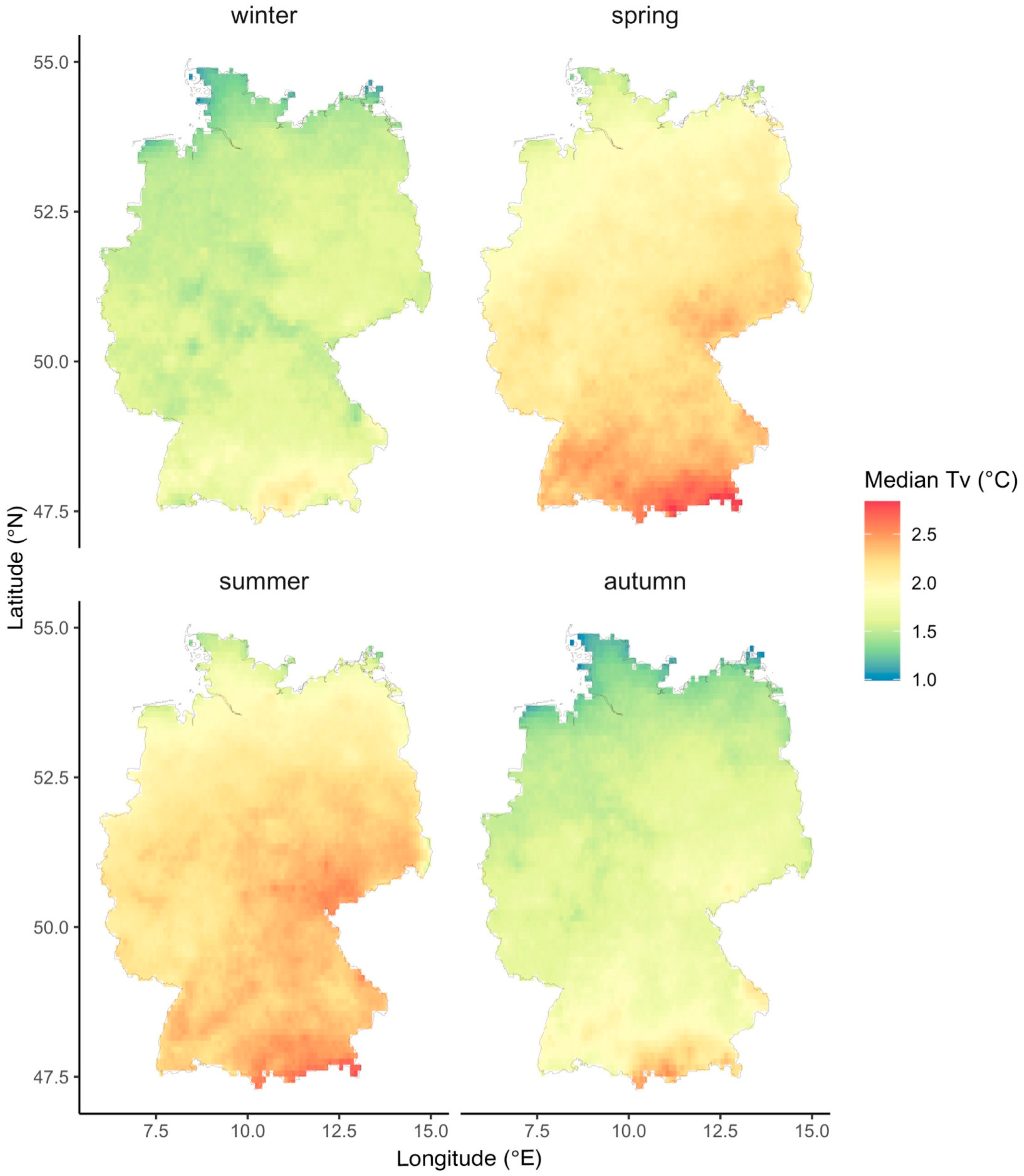
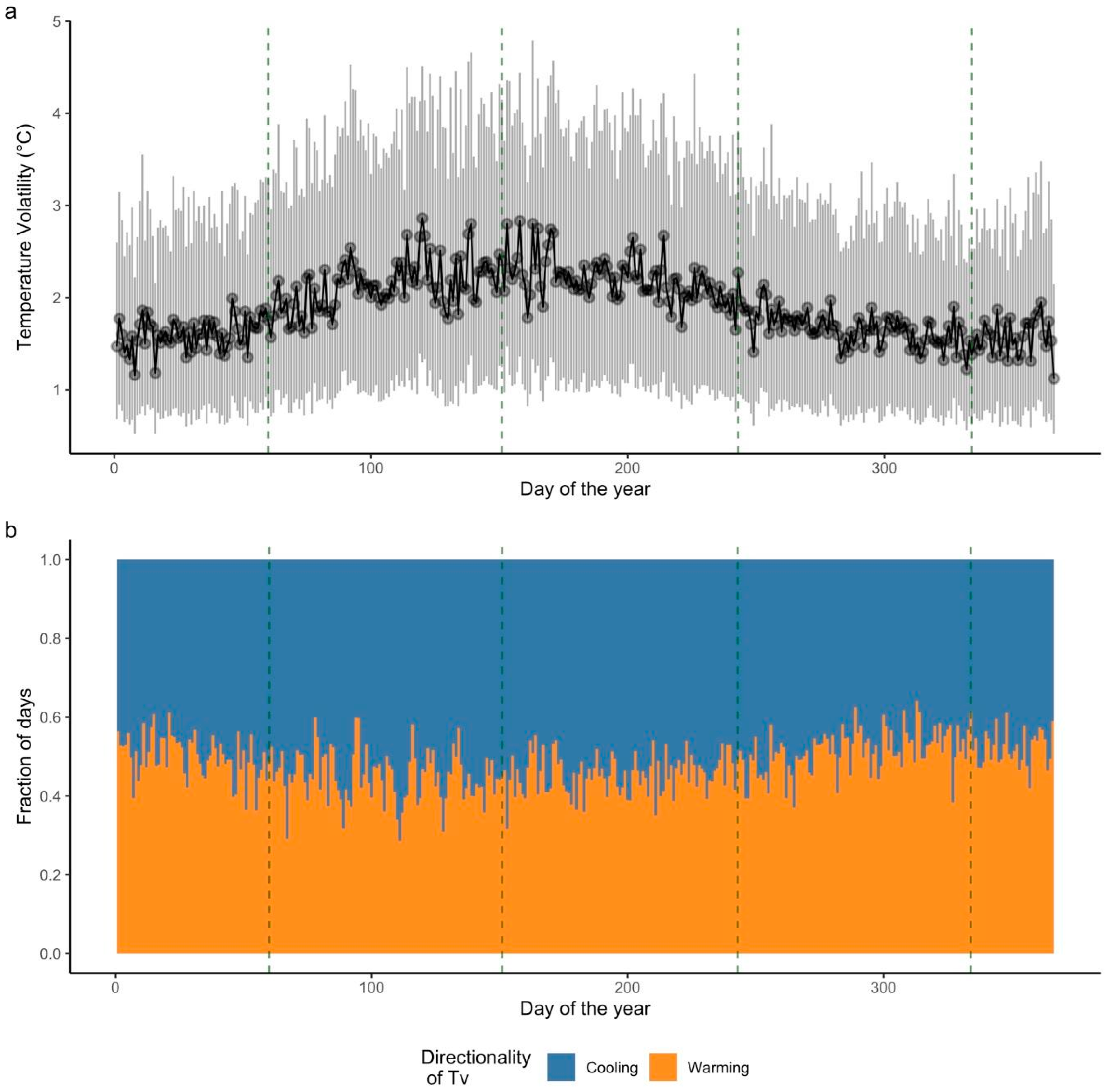
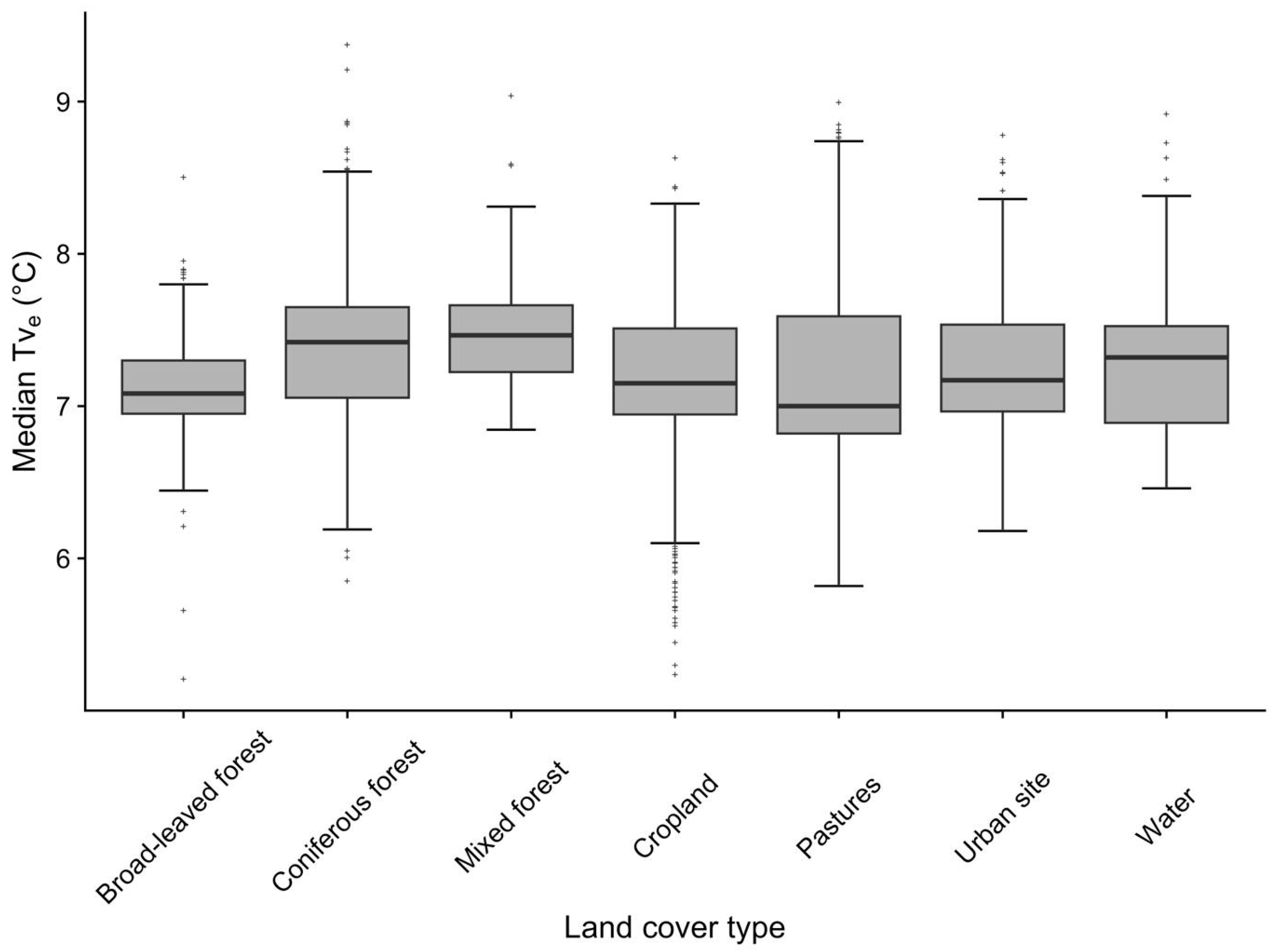
3.1. Temperature Volatility

Figure 1 illustrates the median magnitude of temperature volatility (Tv) across Germany during winter, spring, summer, and autumn from 1990 to 2022. Median Tv increases on a latitudinal gradient north to south during all seasons. Overall, median Tv was higher in spring and summer, ranging from 1.5 °C in the north to over 2.5 °C in the south, compared to autumn and winter (1 °C in the north to about 2.5 °C in the south).

Along with spatial variation, there is also an intra-year variation (i.e., seasonality) of Tv, as shown in Figure 2. The magnitude of median Tv peaked between late spring and early summer, exceeding 2.5 °C, and reached its lowest in mid-winter at about 1.2 °C (Figure 2a). On average, the percentage of Tv associated with a cooling and warming, respectively, fluctuated around 50 ± 10% throughout the year, indicating a low variation in the directionality of Tv throughout the year (Figure 2b).

3.2. Extreme Temperature Volatility

3.2.1. Magnitude and Seasonality

Similar to the median Tv, the median extreme temperature volatility (Tv_e) also showed both spatial and seasonal variation, as depicted in Figure 3. In each season, median Tv_e increased from north-west to south with further distance from the coast. During the warming half-year (spring, summer), Tv_e showed a latitudinal gradient from 6 to 7 °C near the coast to 9–10 °C in the Alps. Specifically, in spring, median Tv_e exceeded 10 °C at the southern border of Germany, i.e., the Alpine region. Conversely, during the cooling half-year (autumn, winter), the magnitude of the Tv_e was lower than in the spring and summer. While maintaining a similar latitudinal gradient, median Tv_e varied in ranges from <4 °C in the north up to 8–9 °C in the south during winter, and up to 9–10 °C during autumn.

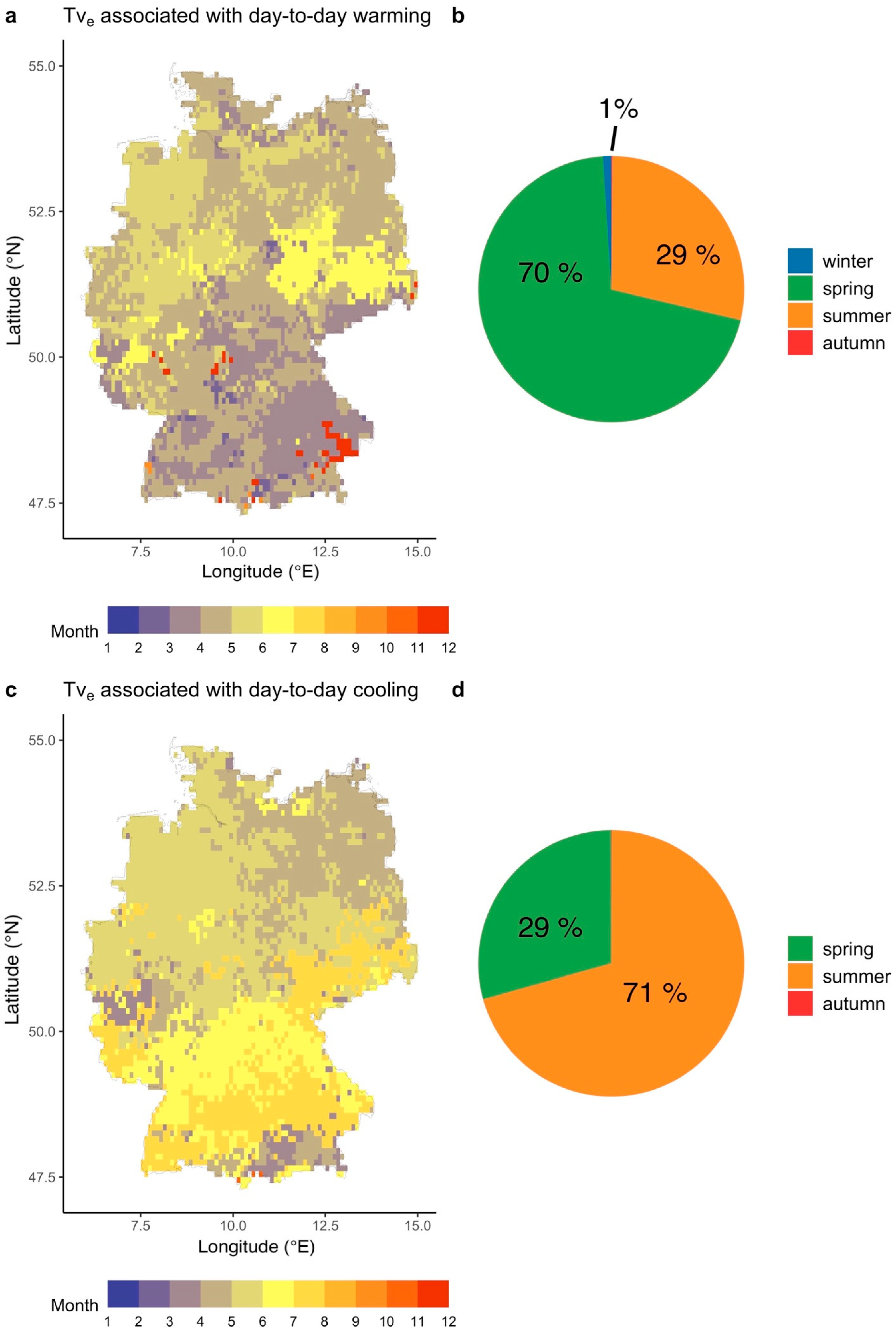
3.2.2. Directionality and Timing

As we analysed absolute values of Tv_e, it was important to examine whether Tv_e indicated a day-to-day cooling or warming (directionality of volatility) as shown in Figure 4, representing the fraction of Tv_e days associated with a day-to-day warming across Germany in different seasons. The directionality of Tv_e differed seasonally. In general, the percentage of days associated with extreme day-to-day warming decreased north to south across Germany. In spring, summer, and autumn, up to 60% of the days were associated with warming in the north, whereas this fraction dropped below 20% in the south, indicating that Tv_e is rather connected to sudden cooling during these seasons (shown in Figure S4). However, in winter, days associated with extreme warming predominated in northern and central Germany (exceeding 60% of days) and reached over 40% in the south. The complementary pattern of Tv_e associated with a day-to-day cooling is shown in Figure S4 of the Supplementary Materials section.

Figure 5 shows the timing of Tv_e associated with day-to-day warming throughout the year. In the northern regions, extreme day-to-day warming predominantly occurred in late spring (May) and early summer (June), while in the south, it occurred during early spring (February and March). Notably, Tv_e linked to warming sporadically occurred in late winter or early spring in regions with higher elevation in central and southern Germany (Figure 5a). Overall, extreme day-to-day warming was predominantly observed during the warming seasons in spring (70%) and summer (29%). Only 1% of Tv_e associated with day-to-day warming occurred in winter, and never occurred in autumn (Figure 5b). Conversely, extreme day-to-day cooling showed a reversed appearance throughout the year, with 29% of Tv_e occurring in spring and 71% occurring in summer (Figure 5d). Across Germany, Tv_e associated with day-to-day cooling occurred in late spring (May) and early summer (June) in the north, and during mid and late summer (July, August) in the south. However, in the Alpine region, extreme day-to-day cooling predominantly occurred in early spring (Figure 5c).

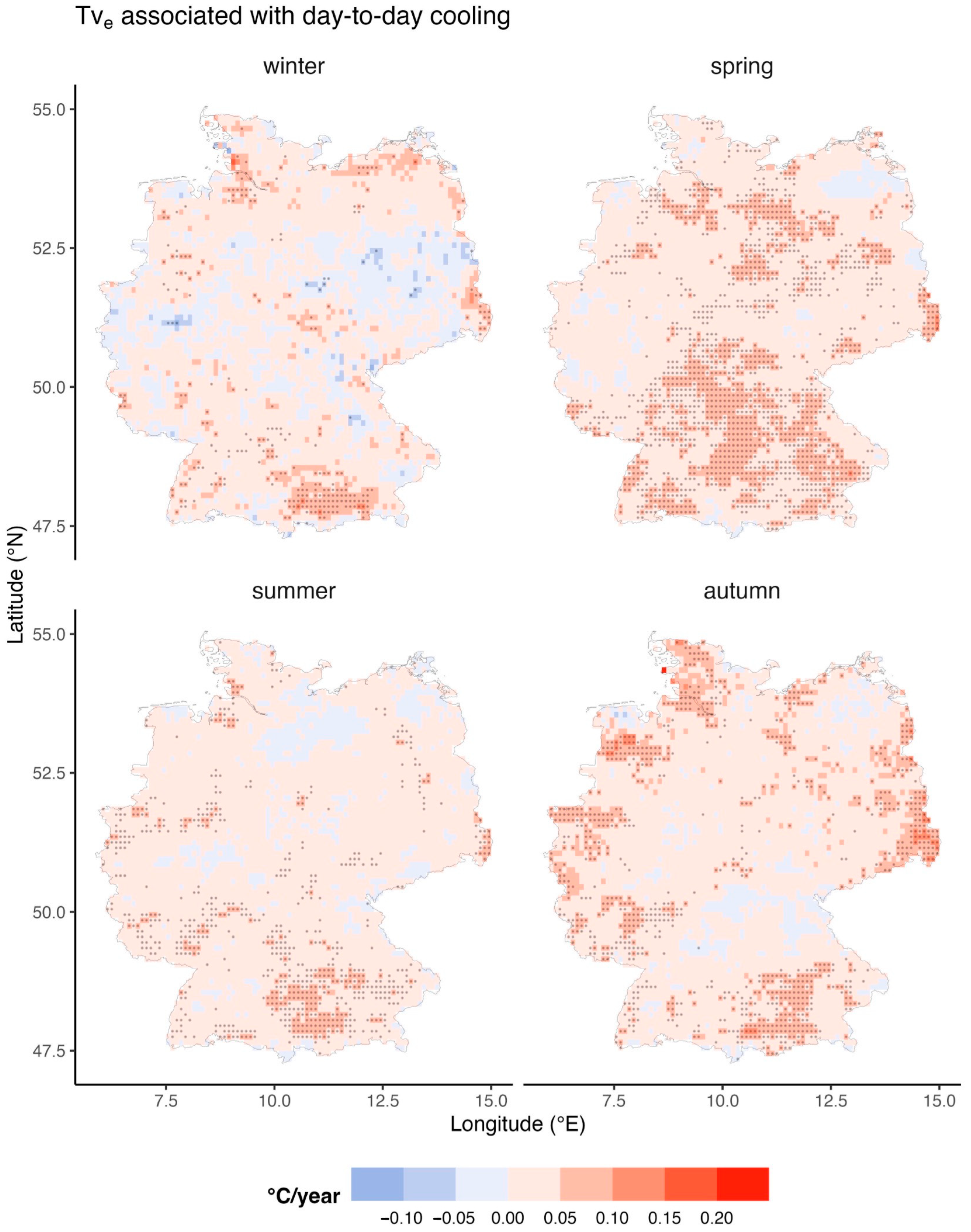
3.3. Trends in Extreme Temperature Volatility

During spring and autumn, large parts of Germany showed an increasing trend in Tv_e (increase in the magnitude of Tv_e) over the 1990–2022 period (Figure S5), while large parts of southern Germany showed a significant (p < 0.05) increasing trend in Tv_e. However, the magnitude of Tv_e decreased or remained unchanged in central and northern Germany (>50° N), as shown in Figure S5. We further partitioned the Tv_e associated with day-to-day warming and cooling, and analysed its seasonal long-term trend over the 1990–2022 period as shown in Figure 6 and Figure 7, respectively.

Over the winter time, median Tv_e associated with warming decreased significantly up to −0.1 °C/year in the north-eastern parts of Germany, while in southern regions, its magnitude significantly increased up to 0.15 °C/year. The magnitude of median Tv_e associated with warming showed a weak and non-significant trend (>−0.05 °C/year and <0.05 °C/year) for most parts of Germany during the spring and summer season. Trends in median Tv_e associated with warming during the autumn showed a strong increase of over 0.26 °C/year, but were only limited to north-eastern Germany. Overall, less than 12% of Germany showed significant trends in Tv_e associated with warming during the 1990–2022 period.

In comparison, Tv_e associated with day-to-day cooling showed a coherent spatial distribution of increasing trends through Germany. Throughout all seasons, significant positive trends (up to 0.15 °C/year) of an increasing magnitude of Tv_e associated with day-to-day cooling were observed in the Alpine region. Especially in spring, the majority (>60%) areas in the south (Latitude < 50° N) showed significant positive trends (magnitude up to 0.15 °C/year) in Tv_e associated with day-to-day cooling. During winter, summer, and autumn, the Tv_e associated with day-to-day cooling largely (>80% area) remained unchanged (i.e., a non-significant trend) over the 1990–2022 period.

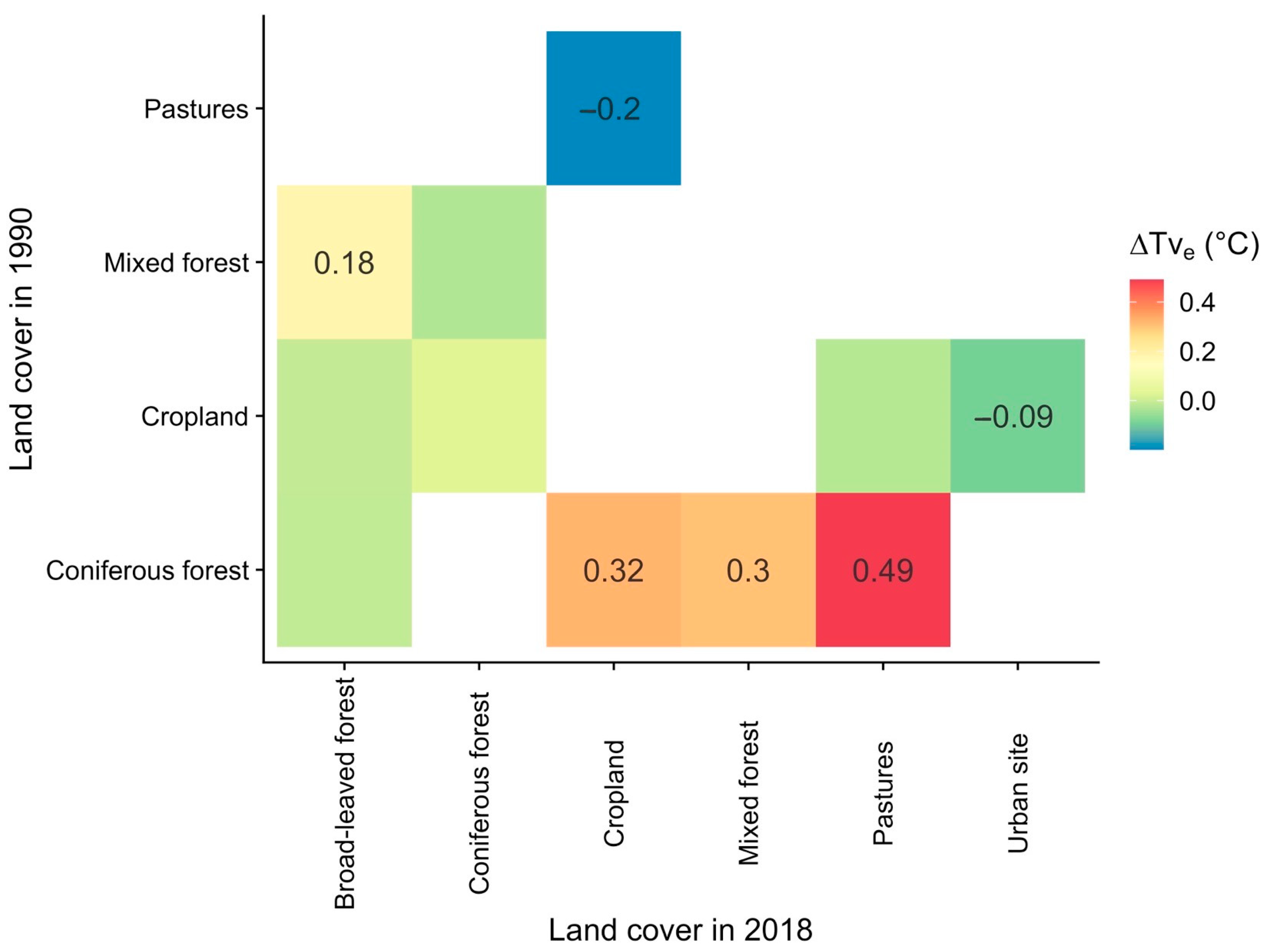
3.4. Impact of Land Use and Land Cover Change on Extreme Temperature Volatility

In Figure 8, we show the distribution (in the form of boxplots) of (temporal) median Tv_e across different land cover types during the 1990–2018 period. Within all land cover types, the median Tv_e predominantly varied between 6 °C and 9 °C. The most pronounced dispersion of median Tv_e was observed over areas designated as pastures, whereas the median Tv_e over mixed and broad-leaved forests showed the least dispersion.

As we show in Figure S6, the highest percent area showing Land Use and Land Cover Change (LULCC) in Germany over the period was transformed from cropland to pastures (24.8%), mixed forest to broad-leaved forest (16.1%) and pastures to cropland (13.4%). Figure 9 shows the change in extreme temperature volatility (∆Tv_e, Equation (3)) associated with LULCC between 1990 and 2018. Most LULCCs were accompanied by an increase in ∆Tv_e. The transformation of coniferous forest into pastures, croplands and mixed forests, respectively, was associated with a significant increase in ∆Tv_e of 0.49 °C, 0.32 °C and 0.3 °C. Contrarily, transforming pastures to cropland and cropland to urban sites was accompanied by a significant decrease in ∆Tv_e of 0.2 °C and 0.09 °C, respectively.

4. Discussion

The main aspect of the study was to investigate extreme day-to-day temperature changes (i.e., extreme temperature volatility) in Germany between 1990 and 2022 with regard to their magnitude, seasonality, timing and directionality. These results were compared to land cover changes in Germany to assess any potential links.

4.1. Trends in Extreme Temperature Volatility

It is striking that even though the global mean surface temperature has been rising over the last decades due to climate change [1], trends in the magnitude of Tv_e across Germany were predominantly insignificant (Figure S5, Figure 6 and Figure 7).

Changes in maximum air temperature can affect land vegetation functioning through multiple pathways and processes. For example, rising air temperature can extend the vegetation growing season [10,11,12,13,43], can lower the surface albedo over a longer period of time due to snow melt, and also affects the ecosystem water balance due to extended high transpiration phases [44]. In this context, in addition to mean temperature, Tx is widely used to study the effects on ecosystems, especially on the start and end of the growing season when plants are particularly sensitive to changes in the temperature [45,46,47].

When facing increasing hot summer extremes, the shift in vegetation phenology might enhance summer droughts, or on the contrary, could balance the local climate through elongated transpiration if water is not a limiting factor [44]. Under these circumstances, the significant positive trend in the magnitude of extreme day-to-day cooling in south Germany, especially during spring, could affect plant development and functioning, and the ecosystem’s carbon and water balance. The potential effect of temperature volatility on plant functioning (e.g., phenology) is likely different to the effect of thermal changes in the environment over longer period, but this has to be investigated more closely. During the past few years (1959 to 2017), late spring frost events have increased in Europe and Asia, mostly affecting temperate broadleaved forests, while frost events have decreased in North America [48]. Leading to tissue damage, late spring frosts have a severe effect on growth, competitive ability, and the distribution limits of plants. This effect is especially strong in spring while leaves are still young and plants more vulnerable [49].

Similar to our results on Tv_e (Figure 4), the changes in mean spring temperature between 1951 and 2015 also showed different temperature trends in northern versus southern Germany [50]. These regional differences could result in the balancing effect of the oceans on climate extremes through a larger thermal inertia, which decreases with a further distance from the coast [50,51,52]. Therefore, the latitudinal trends in both the magnitude and directionality of Tv_e (Figure 3 and Figure 4) could be explained by the topography of Germany and the more maritime climate in the northern lowlands.

Furthermore, rapid changes in the seasonal mean values of extreme air temperature could be linked with changes in the atmospheric circulation regimes [53].

Contrarily to Ombadi and Risser’s [3] study, which showed a clear spatial pattern of the timing of extreme temperature volatility in the US, depending on the topography of the landscape, the spatial pattern in Germany was less coherent. Both extreme day-to-day cooling and warming occurred predominantly during the warming half-year in Germany and did not show a continuous dependency on the topography.

When analysing day-to-day changes in the daily mean temperature in China, Wang et al. [14] found the majority of extreme temperature swings to be occurring from January until July. They explain their findings by mentioning a higher interaction between land and the near-surface air during land surface warming. In contrast to this study, the trends Wang et al. [14] found show a decrease in the range of day-to-day mean temperature variability. This may be rooted in the geographical differences, but also supports the importance of analysing the volatility of daily extreme temperatures, especially as temperature extremes are expected to further increase due to global warming [54].

4.2. Impact of Land Use and Land Cover Changes on Extreme Temperature Volatility

Land cover and land cover changes can have a significant effect on climate on a regional scale [55]. Land cover changes, from natural vegetation to bare ground or cultivated areas, can increase land surface temperatures [18,19]. For example, by replacing coniferous forests with broad-leaved forests across Europe, Tx could be reduced by up to 1.8 °C, as broad-leaved forests in Europe have a higher offsetting effect on hot temperature extremes in summer than coniferous forests [56]. The higher cooling effect of broad-leaved trees on the local climate compared to coniferous species is rooted in a higher albedo and a higher transpiration rate, leading to a larger evaporative cooling effect [57].

In general, forests are found to have a balancing effect on the local climate, caused by their biophysical effects [58]. Evaporative cooling has a damping effect on high temperatures during summer, while the low surface albedo of forested areas causes a mild warming during winter [59,60,61]. Even though the albedo of forests is lower compared to bare ground, and it has a crucial impact on climate on a global scale, the effect of evaporative cooling is found to be a stronger driver of land cover feedback climate on a local scale [62]. Historically, deforestation in Europe influenced local climate by increasing hot temperature extremes, especially caused by reduced humidity and surface roughness [63,64]. Deforestation decreases the surface roughness, lowers the transpiring leaf area, and thereby increases the local diurnal surface temperature range [56,65,66]. This effect can cause a local raise of mean surface temperature of up to 1 °C [62]. Hence, the increase in Tv_e over areas that changed from forest vegetation to agricultural land (Figure 9) could be a consequence of lower evaporative cooling. The increase in Tv_e over areas that changed to mixed forests could be rooted in the significantly lower transpiration rate, and the interception evaporation of young forests compared to old forests was due to a smaller leaf area [67] and a lower bark storage capacity [68].

Overall, local air temperatures tend to be higher in urban areas compared to rural areas, mainly caused by the reduction in evapotranspiration, increase in heat storage (e.g., because of low surface albedo) and anthropogenic heat emissions [69]. Nevertheless, the transformation of croplands to urban sites in Germany from 1990 to 2018 was linked to a decrease of 0.09 °C in Tv_e compared to an unchanged area (Figure 9). As we only examined rapid changes in temperature, regardless of the actual temperature magnitude, urban areas could have a dampening effect on temperature changes because of the larger capacity for heat storage. Future research should further explore these relationships to better understand the complex interactions between temperature volatility, land use changes, and their cumulative effects on local and regional climate systems, particularly in the context of ongoing climate change.

5. Conclusions

In summary, median and extreme temperature volatility increased with further distance from the coast from north to south across Germany. Overall, extreme temperature volatility (Tv_e) was predominantly associated with cooling, except in winter. This trend intensified at a latitudinal gradient north to south. The majority of Tv_e occurred during the warming half-year (March to August). Extreme day-to-day warming mostly occurred during spring, while extreme day-to-day cooling predominantly occurred during summer.

Trends in Tv_e varied regionally and seasonally. Only singular regions of Germany exhibited significant trends in median Tv_e associated with warming over the study period. Significant trends in an increasing magnitude of Tv_e associated with day-to-day cooling occurred in the Alpine region during every season. Generally, LULCC is predominantly linked to a rise in in local Tv_e, probably due to changes in the transpiration rate.

The impact of LULCC on the regional climate and temperature changes is a topic worthy of further investigation regarding climate change, an increasing world population and urbanisation [2].

By evaluating regional extreme temperatures in Germany, this study might contribute to a higher public perception of local climate change consequences.

References

1. IPCC. Climate Change 2021: The Physical Science Basis: Working Group I contribution to the Sixth Assessment Report of the Intergovernmental Panel on Climate Change; Cambridge University Press: Cambridge, UK; New York, NY, USA, 2021. [Google Scholar]
2. IPCC. Climate Change 2023: Synthesis Report. A Report of the Intergovernmental Panel on Climate Change; Contribution of Working Groups I, II and III to the Sixth Assessment Report of the Intergovernmental Panel on Climate Core Writing Team, Lee, H., Romero, J., Eds.; IPCC: Geneva, Switzerland, 2023.
3. Ombadi, M.; Risser, M.D. What’s the temperature tomorrow? Increasing trends in extreme volatility of daily maximum temperature in Central and Eastern United States (1950–2019). Weather Clim. Extrem. 2022, 38, 100515. [Google Scholar] [CrossRef]
4. Lin, H.; Zhang, Y.; Xu, Y.; Xu, X.; Liu, T.; Luo, Y.; Xiao, J.; Wu, W.; Ma, W. Temperature changes between neighboring days and mortality in summer: A distributed lag non-linear time series analysis. PLoS ONE 2013, 8, e66403. [Google Scholar] [CrossRef] [PubMed]
5. Hovdahl, I. The deadly effect of day-to-day temperature variation in the United States. Environ. Res. Lett. 2022, 17, 104031. [Google Scholar] [CrossRef]
6. Guo, Y.; Barnett, A.G.; Yu, W.; Pan, X.; Ye, X.; Huang, C.; Tong, S. A large change in temperature between neighbouring days increases the risk of mortality. PLoS ONE 2011, 6, e16511. [Google Scholar] [CrossRef]
7. Cheng, J.; Zhu, R.; Xu, Z.; Xu, X.; Wang, X.; Li, K.; Su, H. Temperature variation between neighboring days and mortality: A distributed lag non-linear analysis. Int. J. Public Health 2014, 59, 923–931. [Google Scholar] [CrossRef] [PubMed]
8. Kotz, M.; Wenz, L.; Stechemesser, A.; Kalkuhl, M.; Levermann, A. Day-to-day temperature variability reduces economic growth. Nat. Clim. Chang. 2021, 11, 319–325. [Google Scholar] [CrossRef]
9. Badeck, F.W.; Bondeau, A.; Böttcher, K.; Doktor, D.; Lucht, W.; Schaber, J.; Sitch, S. Responses of spring phenology to climate change. New Phytol. 2004, 162, 295–309. [Google Scholar] [CrossRef]
10. Jeong, S.-J.; Ho, C.-H.; Gim, H.-J.; Brown, M.E. Phenology shifts at start vs. end of growing season in temperate vegetation over the Northern Hemisphere for the period 1982–2008. Glob. Chang. Biol. 2011, 17, 2385–2399. [Google Scholar] [CrossRef]
11. Estrella, N.; Menzel, A. Responses of leaf colouring in four deciduous tree species to climate and weather in Germany. Clim. Res. 2006, 32, 253–267. [Google Scholar] [CrossRef]
12. Doi, H.; Takahashi, M. Latitudinal patterns in the phenological responses of leaf colouring and leaf fall to climate change in Japan. Glob. Ecol. Biogeogr. 2008, 17, 556–561. [Google Scholar] [CrossRef]
13. Delpierre, N.; Dufrêne, E.; Soudani, K.; Ulrich, E.; Cecchini, S.; Boé, J.; François, C. Modelling interannual and spatial variability of leaf senescence for three deciduous tree species in France. Agric. For. Meteorol. 2009, 149, 938–948. [Google Scholar] [CrossRef]
14. Wang, X.; Wu, G.; Qin, Y. Day-to-Day Temperature Variability in China During Last 60 Years Relative to Arctic Oscillation. Earth Space Sci. 2022, 9, e2022EA002587. [Google Scholar] [CrossRef]
15. Rebetez, M. Changes in daily and nightly day-to-day temperature variability during the twentieth century for two stations in Switzerland. Theor. Appl. Climatol. 2001, 69, 13–21. [Google Scholar] [CrossRef]
16. Moberg, A.; Jones, P.D.; Barriendos, M.; Bergström, H.; Camuffo, D.; Cocheo, C.; Davies, T.D.; Demarée, G.; Martin-Vide, J.; Maugeri, M.; et al. Day-to-day temperature variability trends in 160- to 275-year-long European instrumental records. JGR Atmos. 2000, 105, 22849–22868. [Google Scholar] [CrossRef]
17. IPCC. Climate Change and Land: An IPCC Special Report on Climate Change, Desertification, Land Degradation, Sustainable Land Management, Food Security, and Greenhouse Gas Fluxes in Terrestrial Ecosystems; IPCC: Cambridge, UK, 2019.
18. Zhang, F.; Tiyip, T.; Kung, H.; Johnson, V.C.; Maimaitiyiming, M.; Zhou, M.; Wang, J. Dynamics of land surface temperature (LST) in response to land use and land cover (LULC) changes in the Weigan and Kuqa river oasis, Xinjiang, China. Arab. J. Geosci. 2016, 9, 499. [Google Scholar] [CrossRef]
19. Merga, B.B.; Moisa, M.B.; Negash, D.A.; Ahmed, Z.; Gemeda, D.O. Land Surface Temperature Variation in Response to Land-Use and Land-Cover Dynamics: A Case of Didessa River Sub-basin in Western Ethiopia. Earth Syst. Environ. 2022, 6, 803–815. [Google Scholar] [CrossRef]
20. DWD. Nationaler Klimareport; DWD: Offenbach, Germany, 2022. [Google Scholar]
21. Federal Statistical Office of Germany. Land- und Forstwirtschaft, Fischerei: Bodenflächen nach Art der Tatsächlichen Nutzung; Reihe 5.1; Federal Statistical Office of Germany: Wiesbaden, Germany, 2022.
22. van der Schrier, G.; van den Besselaar, E.J.M.; Klein Tank, A.M.G.; Verver, G. Monitoring European average temperature based on the E-OBS gridded data set. JGR Atmos. 2013, 118, 5120–5135. [Google Scholar] [CrossRef]
23. Haylock, M.R.; Hofstra, N.; Klein Tank, A.M.G.; Klok, E.J.; Jones, P.D.; New, M. A European daily high-resolution gridded data set of surface temperature and precipitation for 1950–2006. JGR Atmos. 2008, 113. [Google Scholar] [CrossRef]
24. Cornes, R.C.; van der Schrier, G.; van den Besselaar, E.J.M.; Jones, P.D. An Ensemble Version of the E-OBS Temperature and Precipitation Data Sets. JGR Atmos. 2018, 123, 9391–9409. [Google Scholar] [CrossRef]
25. Cornes, R.C.; Jones, P.D. How well does the ERA-Interim reanalysis replicate trends in extremes of surface temperature across Europe? JGR Atmos. 2013, 118. [Google Scholar] [CrossRef]
26. Copernicus Climate Change Service. E-OBS Daily Gridded Meteorological Data for Europe from 1950 to Present Derived from In-Situ Observations; ECMWF: Reading, UK, 2020. [Google Scholar]
27. Copernicus Land Monitoring Service. CORINE Land Cover. Available online: https://land.copernicus.eu/pan-european/corine-land-cover (accessed on 9 June 2023).
28. European Environment Agency. CORINE Land Cover 2018 (Raster 100 m), Europe, 6-Yearly—Version 2020_20u1, May 2020. 2019. Available online: https://land.copernicus.eu/en/products/corine-land-cover/clc2018 (accessed on 9 June 2023).
29. European Environment Agency. CORINE Land Cover 1990 (Raster 100 m), Europe, 6-Yearly—Version 2020_20u1, May 2020. 2019. Available online: https://land.copernicus.eu/en/products/corine-land-cover/clc1990 (accessed on 9 June 2023).
30. Hijmans, R. terra: Spatial Data Analysis, R Package Version 1.7-80. 2023. Available online: https://CRAN.R-project.org/package=terra (accessed on 11 July 2024).
31. Hijmans, R. raster: Geographic Data Analysis and Modeling, R Package Version 3.6-20. 2023. Available online: https://CRAN.R-project.org/package=raster (accessed on 11 July 2024).
32. Kosztra, B.; Büttner, G.; Hazeu, G.; Arnold, S. Updated CLC Illustration Nomenclature Guidelines. Available online: https://land.copernicus.eu/user-corner/technical-library/corine-land-cover-nomenclature-guidelines/docs/pdf/CLC2018_Nomenclature_illustrated_guide_20190510.pdf (accessed on 9 June 2023).
33. Miller, J.; Miller, J.C. Statistics and Chemometrics for Analytical Chemistry, 6th ed.; Pearson Education Ltd.: Essex, UK, 2014; ISBN 978-0-273-73042-2. [Google Scholar]
34. Hamed, K.H. Exact distribution of the Mann–Kendall trend test statistic for persistent data. J. Hydrol. 2009, 365, 86–94. [Google Scholar] [CrossRef]
35. Kendall, M.G.; Gibbons, J.D. Rank Correlation Methods; Arnold: London, UK, 1990. [Google Scholar]
36. Mann, H.B. Nonparametric Tests Against Trend. Econometrica 1945, 13, 245. [Google Scholar] [CrossRef]
37. Kong, D.; Song, H. rtrend: Trend Estimating Tools, R Package Version 0.1.4. 2022. Available online: https://cran.r-project.org/web/packages/rtrend/rtrend.pdf (accessed on 9 April 2023).
38. Wilks, D.S. “The Stippling Shows Statistically Significant Grid Points”: How Research Results are Routinely Overstated and Overinterpreted, and What to Do about It. Bull. Am. Meteorol. Soc. 2016, 97, 2263–2273. [Google Scholar] [CrossRef]
39. Wickham, H.; François, R.; Henry, L.; Müller, K.; Vaughan, D. dplyr: A Grammar of Data Manipulation. 2023. Available online: https://dplyr.tidyverse.org (accessed on 11 July 2024).
40. Grolemund, G.; Wickham, H. Dates and Times Made Easy with lubridate. J. Stat. Soft. 2011, 40. [Google Scholar] [CrossRef]
41. Wickham, H. Ggplot2: Elegrant Graphics for Data Analysis, 2nd ed.; Springer: Cham, Switzerland, 2016. [Google Scholar]
42. ESRI Data and Maps. World Countries Generalized. Available online: https://hub.arcgis.com/datasets/esri::world-countries-generalized/about (accessed on 11 July 2024).
43. Marqués, L.; Hufkens, K.; Bigler, C.; Crowther, T.W.; Zohner, C.M.; Stocker, B.D. Acclimation of phenology relieves leaf longevity constraints in deciduous forests. Nat. Ecol. Evol. 2023, 7, 198–204. [Google Scholar] [CrossRef] [PubMed]
44. Peñuelas, J.; Rutishauser, T.; Filella, I. Ecology. Phenology feedbacks on climate change. Science 2009, 324, 887–888. [Google Scholar] [CrossRef]
45. Sun, M.; Li, P.; Ren, P.; Tang, J.; Zhang, C.; Zhou, X.; Peng, C. Divergent response of vegetation phenology to extreme temperatures and precipitation of different intensities on the Tibetan Plateau. Sci. China Earth Sci. 2023, 66, 2200–2210. [Google Scholar] [CrossRef]
46. Ren, P.; Liu, Z.; Zhou, X.; Peng, C.; Xiao, J.; Wang, S.; Li, X.; Li, P. Strong controls of daily minimum temperature on the autumn photosynthetic phenology of subtropical vegetation in China. For. Ecosyst. 2021, 8, 31. [Google Scholar] [CrossRef]
47. Li, C.; Zou, Y.; He, J.; Zhang, W.; Gao, L.; Zhuang, D. Response of Vegetation Phenology to the Interaction of Temperature and Precipitation Changes in Qilian Mountains. Remote Sens. 2022, 14, 1248. [Google Scholar] [CrossRef]
48. Zohner, C.M.; Mo, L.; Renner, S.S.; Svenning, J.-C.; Vitasse, Y.; Benito, B.M.; Ordonez, A.; Baumgarten, F.; Bastin, J.-F.; Sebald, V.; et al. Late-spring frost risk between 1959 and 2017 decreased in North America but increased in Europe and Asia. Proc. Natl. Acad. Sci. USA 2020, 117, 12192–12200. [Google Scholar] [CrossRef]
49. Vitra, A.; Lenz, A.; Vitasse, Y. Frost hardening and dehardening potential in temperate trees from winter to budburst. New Phytol. 2017, 216, 113–123. [Google Scholar] [CrossRef] [PubMed]
50. Waldau, T.; Chmielewski, F.-M. Spatial and temporal changes of spring temperature, thermal growing season and spring phenology in Germany 1951–2015. metz 2018, 27, 335–342. [Google Scholar] [CrossRef]
51. Rapp, J. Regionale Klimatrends in Deutschland im 20. Jahrhundert. In Klimastatusbericht 2001; DWD: Offenbach, Germany, 2002. [Google Scholar]
52. Jaagus, J.; Briede, A.; Rimkus, E.; Remm, K. Variability and trends in daily minimum and maximum temperatures and in the diurnal temperature range in Lithuania, Latvia and Estonia in 1951–2010. Theor. Appl. Climatol. 2014, 118, 57–68. [Google Scholar] [CrossRef]
53. Jones, R.N.; Ricketts, J.H. Regime Changes in Atmospheric Moisture under Climate Change. Atmosphere 2022, 13, 1577. [Google Scholar] [CrossRef]
54. Seneviratne, S.I.; Zhang, X.; Adnan, M.; Badi, W.; Dereczynski, C.; Di Luca, A.; Ghosh, S.; Iskandar, I.; Kossin, J.; Lewis, S.; et al. Weather and Climate. In Climate Change 2021—The Physical Science Basis: Contribution of Working Group I to the Sixth Assessment Report of the Intergovernmental Panel on Climate; Masson-Delmotte, V., Zhai, P., Pirani, A., Connors, S.L., Péan, C., Berger, S., Caud, N., Chen, Y., Goldfarb, L., Gomis, M.I., et al., Eds.; Cambridge University Press: Cambridge, UK; New York, NY, USA, 2021; pp. 1513–1766. [Google Scholar]
55. Feddema, J.J.; Oleson, K.W.; Bonan, G.B.; Mearns, L.O.; Buja, L.E.; Meehl, G.A.; Washington, W.M. The importance of land-cover change in simulating future climates. Science 2005, 310, 1674–1678. [Google Scholar] [CrossRef]
56. Duveiller, G.; Hooker, J.; Cescatti, A. The mark of vegetation change on Earth’s surface energy balance. Nat. Commun. 2018, 9, 679. [Google Scholar] [CrossRef]
57. Schwaab, J.; Davin, E.L.; Bebi, P.; Duguay-Tetzlaff, A.; Waser, L.T.; Haeni, M.; Meier, R. Increasing the broad-leaved tree fraction in European forests mitigates hot temperature extremes. Sci. Rep. 2020, 10, 14153. [Google Scholar] [CrossRef] [PubMed]
58. Lawrence, D.; Coe, M.; Walker, W.; Verchot, L.; Vandecar, K. The Unseen Effects of Deforestation: Biophysical Effects on Climate. Front. For. Glob. Chang. 2022, 5, 756115. [Google Scholar] [CrossRef]
59. Schultz, N.M.; Lawrence, P.J.; Lee, X. Global satellite data highlights the diurnal asymmetry of the surface temperature response to deforestation. JGR Biogeosci. 2017, 122, 903–917. [Google Scholar] [CrossRef]
60. Li, Y.; Zhao, M.; Motesharrei, S.; Mu, Q.; Kalnay, E.; Li, S. Local cooling and warming effects of forests based on satellite observations. Nat. Commun. 2015, 6, 6603. [Google Scholar] [CrossRef]
61. Davin, E.L.; de Noblet-Ducoudré, N. Climatic Impact of Global-Scale Deforestation: Radiative versus Nonradiative Processes. J. Clim. 2010, 23, 97–112. [Google Scholar] [CrossRef]
62. Pongratz, J.; Schwingshackl, C.; Bultan, S.; Obermeier, W.; Havermann, F.; Guo, S. Land Use Effects on Climate: Current State, Recent Progress, and Emerging Topics. Curr. Clim. Chang. Rep. 2021, 7, 99–120. [Google Scholar] [CrossRef]
63. Lejeune, Q.; Davin, E.L.; Gudmundsson, L.; Winckler, J.; Seneviratne, S.I. Historical deforestation locally increased the intensity of hot days in northern mid-latitudes. Nat. Clim. Chang. 2018, 8, 386–390. [Google Scholar] [CrossRef]
64. Findell, K.L.; Berg, A.; Gentine, P.; Krasting, J.P.; Lintner, B.R.; Malyshev, S.; Santanello, J.A.; Shevliakova, E. The impact of anthropogenic land use and land cover change on regional climate extremes. Nat. Commun. 2017, 8, 989. [Google Scholar] [CrossRef] [PubMed]
65. Winckler, J.; Reick, C.H.; Luyssaert, S.; Cescatti, A.; Stoy, P.C.; Lejeune, Q.; Raddatz, T.; Chlond, A.; Heidkamp, M.; Pongratz, J. Different response of surface temperature and air temperature to deforestation in climate models. Earth Syst. Dynam. 2019, 10, 473–484. [Google Scholar] [CrossRef]
66. Alkama, R.; Cescatti, A. Biophysical climate impacts of recent changes in global forest cover. Science 2016, 351, 600–604. [Google Scholar] [CrossRef]
67. Martin, T.; Brown, K.; Kučera, J.; Meinzer, F.; Sprugel, D.; Hinckley, T. Control of transpiration in a 220-year-old Abies amabilis forest. For. Ecol. Manag. 2001, 152, 211–224. [Google Scholar] [CrossRef]
68. Brantley, S.T.; Miniat, C.F.; Bolstad, P.V. Rainfall partitioning varies across a forest age chronosequence in the southern Appalachian Mountains. Ecohydrology 2019, 12, e2081. [Google Scholar] [CrossRef]
69. Leal Filho, W.; Wolf, F.; Castro-Díaz, R.; Li, C.; Ojeh, V.N.; Gutiérrez, N.; Nagy, G.J.; Savić, S.; Natenzon, C.E.; Quasem Al-Amin, A.; et al. Addressing the Urban Heat Islands Effect: A Cross-Country Assessment of the Role of Green Infrastructure. Sustainability 2021, 13, 753. [Google Scholar] [CrossRef]
Figure 1. Median temperature volatility (Tv) across Germany during the winter (DJF), spring (MAM), summer (JJA), and autumn (SON) seasons, spanning the 1990–2022 period. Tv is calculated based on Equation (1).
Atmosphere 15 00838 g001
Figure 2. Seasonality (1990–2022) of the (a) magnitude and (b) directionality of the temperature volatility over Germany. The points (top figure) represent median Tv over 1990–2022 period, whereas the error bars represent the 25th and 75th percentile (representing the interquartile range) of Tv during the 1990–2021 period over the whole of Germany. The bar plots in ‘b’ indicate the percentage of Germany showing Tv associated with either cooling or warming.
Atmosphere 15 00838 g002
Figure 3. Median magnitude of extreme temperature volatility (Tve) across Germany during the winter (DJF), spring (MAM), summer (JJA), and autumn (SON) seasons spanning 1990–2022. The Tve is detected based on Equation (2).
Atmosphere 15 00838 g003
Figure 4. Fraction of extreme temperature volatility associated with day-to-day warming during different seasons, i.e., winter (DJF), spring (MAM), summer (JJA), and autumn (SON) across Germany from 1990 to 2022.
Atmosphere 15 00838 g004
Figure 5. Major timing of Tve and its percentage seasonal distribution associated with day-to-day warming (top; (a,b)) and cooling (bottom; (c,d)) during different seasons across Germany from 1990 to 2022.
Atmosphere 15 00838 g005
Figure 6. Mann–Kendall trend (1990–2022) of (yearly) median Tve associated with day-to-day warming across different seasons, i.e., winter (DJF), spring (MAM), summer (JJA), and autumn (SON) in Germany. The grid cell showing significant trend (p < 0.05) is represented by black dots.
Atmosphere 15 00838 g006
Figure 7. Mann–Kendall trend (1990–2022) of (yearly) median Tve associated with day-to-day cooling across different season, i.e., winter (DJF), spring (MAM), summer (JJA), and autumn (SON) in Germany. The grid cell showing significant trend (p < 0.05) is represented by black dots.
Atmosphere 15 00838 g007
Figure 8. Median extreme temperature volatility (Tve) across different land cover types in Germany during the 1990–2022 period.
Atmosphere 15 00838 g008
Figure 9. Change in extreme temperature volatility (∆Tve) associated with land use land cover change (LULCC) in Germany during 1990 and 2018.
Atmosphere 15 00838 g009
Disclaimer/Publisher’s Note: The statements, opinions and data contained in all publications are solely those of the individual author(s) and contributor(s) and not of MDPI and/or the editor(s). MDPI and/or the editor(s) disclaim responsibility for any injury to people or property resulting from any ideas, methods, instructions or products referred to in the content.