Abstract
Using a reanalysis dataset, this work investigates the possible connection of winter East Asia (EA) flow patterns to stratospheric polar vortex (SPV) anomalies. Cluster analysis is performed on the principal components of daily 500 hPa geopotential height fields to identify five distinct flow patterns. SPV anomalies are considered in terms of the occurrence of major sudden stratospheric warmings (MSSWs). The results reveal that for the 15 days before the MSSWs, one of the five patterns occurs more frequently than usual, whereas another occurs less frequently. The former constructively interferes with the climatological EA trough in the troposphere and strengthens the planetary wave activity (heat flux) in the extratropical troposphere and stratosphere. It has a similar pattern in the 500 hPa height to the composite leading to the MSSWs, implying that such strengthening can contribute to the forcing of the MSSWs. The latter is in the opposite sense (destructive interference) and is disadvantageous before the MSSWs. Evidence of a stratospheric downward influence on the five flow patterns is relatively unclear. These results suggest a potential coupling between flow patterns or weather regimes in different regions through the SPV, as well as warrant further investigation of the downward influence on EA weather regimes.
1. Introduction
The extratropical stratosphere and troposphere dynamically couple in both upward and downward directions in connection with anomalous states of the stratospheric polar vortex (SPV) during cold seasons for each hemisphere, i.e., mainly winter for the Northern Hemisphere and spring for the Southern Hemisphere [1,2]. The most striking examples of anomalous SPV states are major sudden stratospheric warmings (MSSWs), in which the SPV experiences rapid and large warming with strong deceleration or even reversal of the zonal mean westerly wind in the extratropical stratosphere [3].
The upward coupling is contributed by the upward propagation of planetary waves [4,5]. Weak SPV states tend to be preceded by enhanced planetary wave activity in the lower stratosphere and troposphere [6,7]. The enhancement in the troposphere is contributed by circulation anomalies in several regions, which essentially act to enhance the climatological planetary wave pattern [8,9,10,11]. In addition, SPV states may need to be preconditioned to accept a pulse of wave activity. The clarification of these two views, including their relative contributions, remains open [1,3].
The downward coupling is a relatively contemporary view and has attracted considerable research attention. The downward coupling in the Northern Hemisphere has often been investigated in the framework of the Northern Annular Mode (NAM). On average, anomalous tropospheric and surface conditions following weak SPV states, such as MSSWs, are characterized by the negative phase of the NAM that is accompanied by high-pressure anomalies over high latitudes and an equatorward shift of the eddy-driven jet in weeks to months after [2]. The opposite is true for strong SPV states.
The average view has been extended by considering extreme states and case-to-case variations. Extreme states or phenomena at the surface following MSSWs include cold air outbreaks over both land (particularly over Northern Eurasia) and oceans (North Atlantic and Arctic Oceans) associated with extreme cold daily minimum and maximum temperatures [12,13,14,15]. The latter, i.e., marine cold air outbreaks, are also associated with strong surface winds over the Labrador Sea and the Greenland–Iceland–Norwegian Seas [16]. The equatorward shift of the jet is concomitant with that of the storm track over the North Atlantic region, increasing the risk of flooding in the Mediterranean and dry spells in some parts of Scandinavia and British Isles [15].
The downward coupling feature, or tropospheric response, also exhibits considerable case-to-case variations among MSSWs in terms of timing, strength, and location, as suggested by [17]. Such variations can arise from several factors. First, the characteristics of MSSWs, such as their strength, persistence, and SPV geometry (e.g., displacement or split), may affect the downward coupling. In particular, the persistence of lower stratospheric anomalies has been found to play an important role [18,19]. Second, extensive studies point out the importance of preceding anomalies in the troposphere [20,21]. Third, preceding anomalies in the ocean also play a role [22]. These factors may be further influenced by the remote forcing of external conditions such as the El Niño/Southern Oscillation and the Quasi-Biennial Oscillation [23].
The role of preceding tropospheric anomalies may be better understood from the perspective of weather regimes, which are recurrent and persistent patterns in large-scale circulation [24]. The influence of the lower SPV state on the weather regimes over the North Atlantic region has been studied to find the highest sensitivity of the negative phase of the North Atlantic Oscillation (NAO), which is characterized by its higher frequency following weak SPV conditions [25]. Domeisen et al. [26] further characterized the tropospheric response to MSSWs over the North Atlantic–European region and identified the Greenland blocking and Atlantic trough regimes as the most frequent patterns in weeks following MSSWs. Lee et al. [27] similarly examined regimes across North America.
Although the downward coupling around the North Atlantic region has attracted considerable attention, the coupling around the Pacific region, including East Asia (EA), is relatively unclear and unexplored [13,28,29]. Nishii et al. [30] reported the cooling of the wintertime Arctic stratosphere via the Western Pacific teleconnection pattern. Jeong et al. [31] highlighted a precursory signal in the stratosphere before a cold surge occurrence in EA. Zhang et al. [32] reported that the MSSW in early January 2021 played a role in inducing the subsequent cold wave in EA. Weather regimes, i.e., large-scale flow patterns, over EA have been identified by Matsueda and Kyouda [33]; however, their possible connection to anomalous SPV states remains unexamined.
Using a reanalysis dataset, we apply an analysis method similar to that introduced in a previous study [33] to the large-scale tropospheric flow patterns over EA and examine changes in their occurrence probability with anomalous SPV states. Anomalous SPV states are considered in terms of MSSW occurrence. Therefore, we explore, from the regime perspective, a possible connection of tropospheric anomalies over EA to SPV states.
2. Data and Analyses
2.1. Data
We employ daily averages (2.5° latitude × 2.5° longitude resolution) of the JRA-55 reanalysis data [34]. The analysis period comprises 45 winters from 1978/1979 to 2022/2023. We mainly analyze the following quantities: zonal mean zonal wind (U) at 60° N, 10 and 100 hPa (U10 and U100, respectively), heat flux (HF) of zonal wavenumbers 1–3 over 45–75° N, 100 hPa (HF100), and geopotential height (Z) at 500 hPa (Z500).
The climatology of each quantity is calculated as the time mean over the 45 years for each of the 366 days including the leap day, which is further smoothed in time using all months at each grid point by retaining only up to the third Fourier mode. Anomalies are calculated as deviations from the daily climatology and are denoted by adding a subscript “a”, e.g., U10a.
2.2. Analyses
To extract dominant flow patterns in the troposphere over EA, we perform a cluster analysis similar to that introduced in [33]. Specifically, we first apply an empirical orthogonal function (EOF) analysis to the daily Z500a fields from November to March (NDJFM) over a region of 20–60° N and 100–170° E. The Z500a fields are weighted with the square root of the cosine of latitude in the EOF analysis. We then apply K-means clustering to the principal components of the 20 leading EOFs, with five clusters. It will turn out later that our results reasonably reproduce the five flow patterns identified in [33]. The five flow patterns are denoted as FPi, where i = 1–5. Each day during NDJFM is assigned to one of the five flow patterns.
We examine the occurrence probability of each FPi, denoted as POi. POi is defined as POi = Fi/N, where N is the total number of specified target days from December to February (DJF), and Fi denotes the number of days for FPi in N. Note that the sum of POi for i is equal to 1 when considering all N days.
We relate the occurrence of the five flow patterns to that of MSSWs, which are identified as a reversal of U10 during DJF, by Charlton and Polvani [35]. The date when U10 becomes negative is referred to as the central date of the MSSW and also as lag = 0 days. To avoid double counting a single event, it is also required that U10 must remain westerly for 20 days before any central date. We use all MSSWs identified above without judging whether or not each MSSW is a final warming. We define a pre-MSSW period (PRE) as lag = −15 to −1 days, and a post-MSSW period (POST) as lag = 0 to +30 days. These periods are based on the characteristic sequence of variability around MSSWs introduced in Section 1, and composite analysis results shown later in this study. POi is obtained for each of the PRE and POST periods by subsampling all DJF days that fall in the PRE or POST period of each MSSW.
The statistical significance of SPV-dependent differences in POi is evaluated using a bootstrap method, in which the MSSW central dates are randomly sorted in terms of year to calculate POi. This procedure is repeated 1000 times to obtain a probability distribution function (PDF) of 1000 artificial values of POi, when it is assumed to be independent of the MSSWs. The actual difference is compared to examine whether it exceeds the 95% interval of the PDF.
3. Results
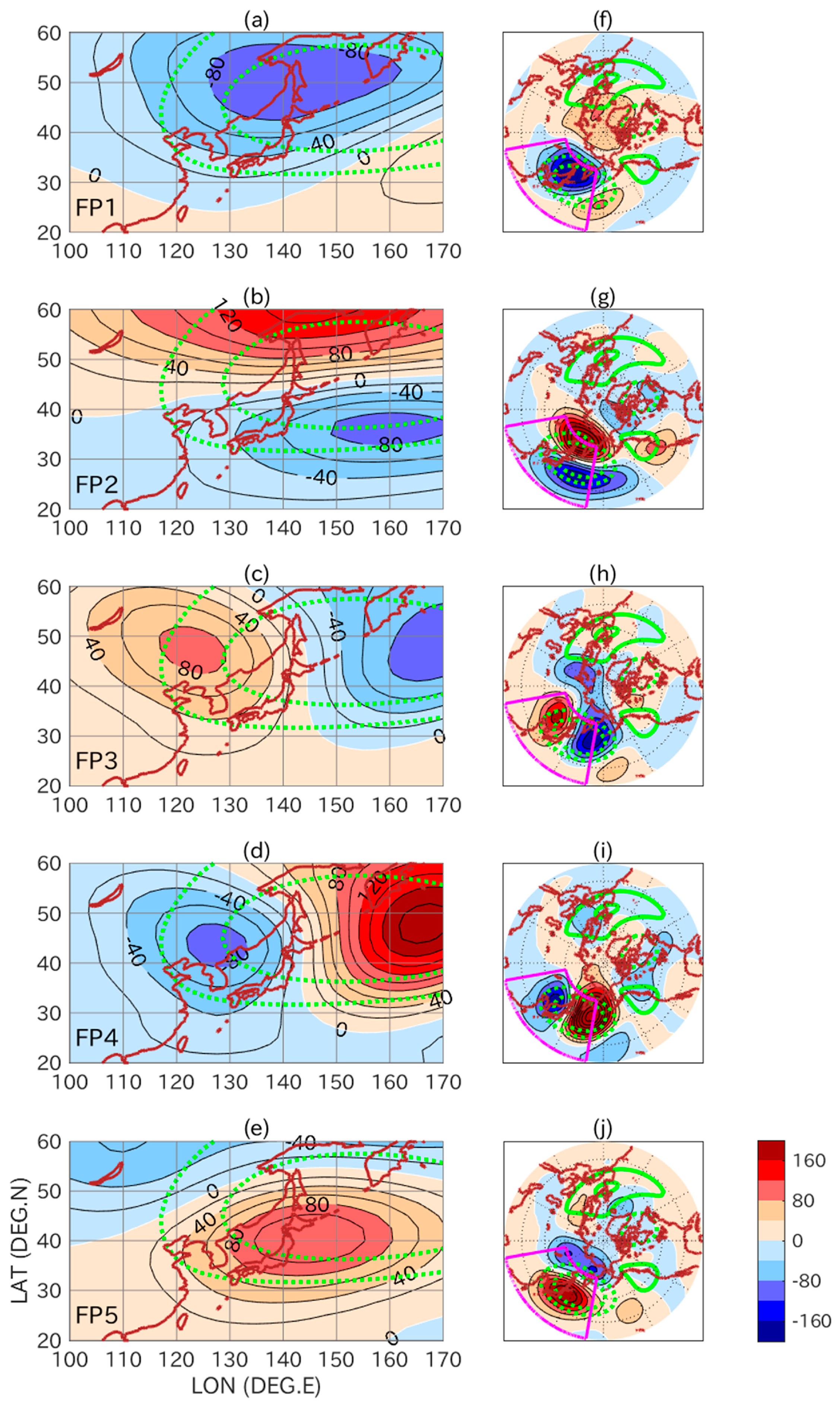
Figure 1a–e shows composite Z500a maps of the five flow patterns. Our results reproduce their spatial patterns obtained in [33], which refer to the five flow patterns as the Winter Monsoon, Western Pacific, High Pressure, Low Pressure, and Southerly Flow patterns, corresponding to Figure 1a–e, respectively. In this study, we refer to the five patterns as FP1–FP5 for simplicity. FP1 exhibits negative Z500a north of the Japanese islands. FP2 is characterized by a meridional dipole pattern of Z500a, with positive values in the north and negative values in the south. FP3 and FP4 exhibit zonal dipole patterns, which are roughly in the opposite phase to each other. FP5 is dominated by positive Z500a in the region. Notably, the negative Z500a in FP1 is in phase with the climatological trough over EA (constructive interference), thereby strengthening the planetary wave. FP2 weakens the climatological trough at higher latitudes (destructive interference) and strengthens it at lower latitudes.
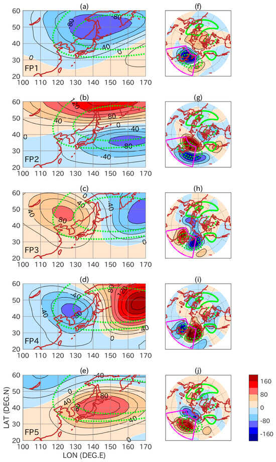
Figure 1.
Composite Z500a maps for each FPi during DJF; FP1–FP5 are shown in (a–e), respectively. Panels (f–j) are similar but plot a hemispheric-scale distribution. Green contours plot the DJF climatological Z500 waves 1–3 pattern, drawn at ±75 and ±150 m. Solid contours represent positive values, and dotted contours negative values. The EA region is marked by violet lines in (f–j).
The average POi values for FP1–FP5 during DJF are 25.1%, 18.2%, 23.8%, 13.1%, and 19.9%, respectively. Similarly, the average persistence values are 3.8, 4.5, 3.5, 2.5, and 2.9 days. The differences in the probability and persistence among the flow patterns are also similar to those reported in [33]. The referenced study [33] mentioned preferred circuits of the patterns as FP1 (FP2)→FP3→FP5→FP4→FP1 (FP2) with a mean time length of approximately 10–11 days, and some transitions, such as between FP4 and FP5, indicating repeated eastward propagation of low-pressure systems.
We examine POi in connection with MSSW occurrence after identifying 26 MSSWs in the target period and confirming their basic features. Figure 2 plots the time evolutions of the U10a and U100a indexes (Figure 2a) and the HF100a index (Figure 2b) composited with respect to the MSSW central date (lag = 0 days). One can confirm that the U10a index shows strongly negative values of more than 30 m/s, i.e., weak SPV states, in the middle stratosphere around lag = 0 days, which correspond to the reversal of U10 by construction. The U100a index also exhibits negative values after around lag = −15 days, which persist at least up to lag = +60 days, with a peak around lag = +20 days. The HF100a index shows an anomalously strong heat flux, i.e., an increased wave activity flux (in the vertical component) in the extratropical lower stratosphere, which peaks just before lag = 0 days. These are well-known features of MSSWs, consistent with previous studies [6,7]. Based on Figure 2a,b, we define the PRE period as lag = −15 to −1 days, when the HF100a index is strongly positive, and the POST period as lag = 0 to +30 days, when the U100a index is strongly negative. Notably, the U100a index is already negative for the PRE period.
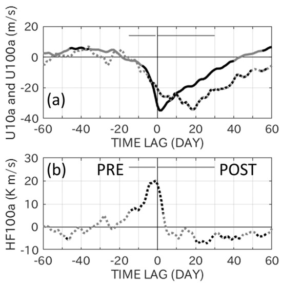
Figure 2.
(a) Composite time series of U10a (m/s, solid line) and U100a (m/s, dotted line, multiplied by 5) with respect to the MSSW central date. (b) Same as (a), but for HF100a (K m/s). Values of statistical significance at the 95% confidence level according to the two-sided t-test are highlighted in black. The PRE and POST periods are denoted in the panels.
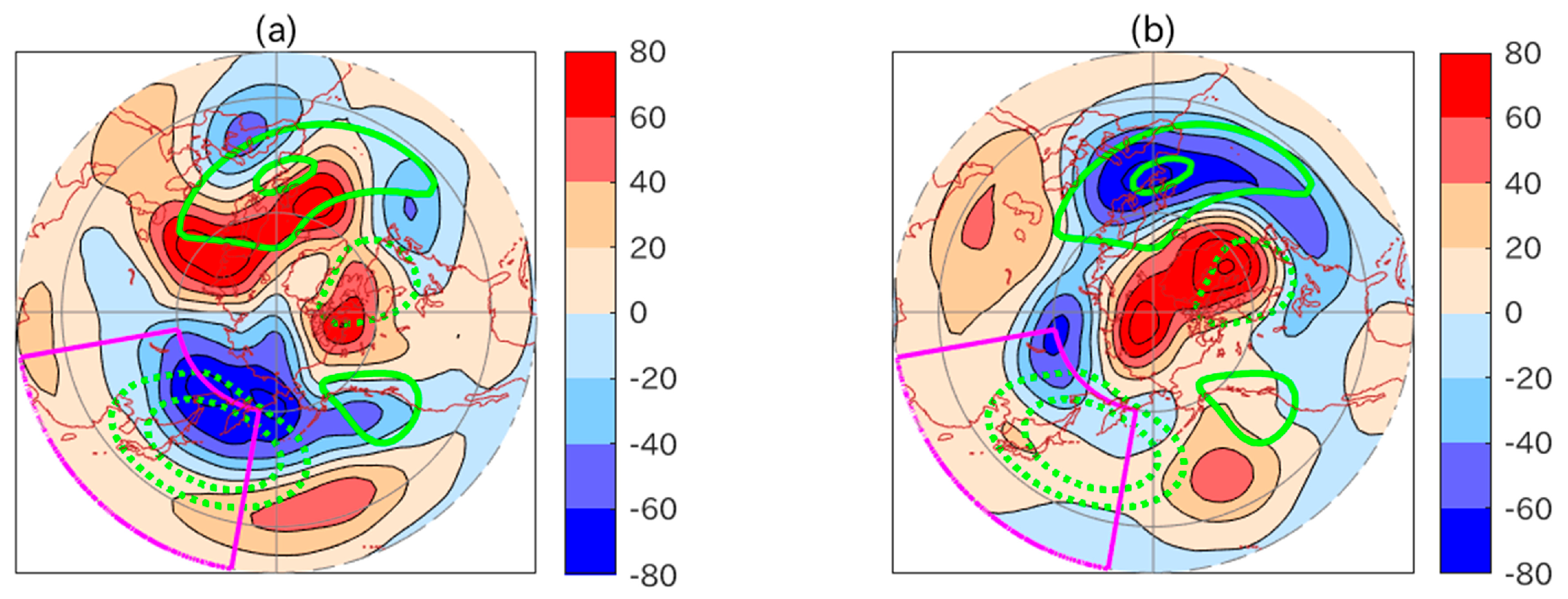
Figure 3 shows composite Z500a maps for each of the PRE and POST periods. The PRE composite map is characterized by negative Z500a over EA and the Northwest Pacific and positive Z500a over Northern Europe and the North Atlantic. These anomalies act to strengthen the climatological planetary wave pattern in the troposphere through constructive interference consistent with the increased HF (Figure 2b). The negative Z500a values also imply a poleward shift of the negative extremum. The POST composite map, in particular, includes positive values over Northeastern Canada and Greenland and negative values over their southern side, including Europe, reminiscent of the negative phase of the NAM. These features for the PRE and POST periods agree with previous studies [9,11,13,29,36].

We sample the occurrence of the five flow patterns FPi and calculate POi for each of the PRE and POST periods (Figure 4). It is important to notice an increased probability of PO1 and a decreased probability of PO2 for the PRE period. The increase in PO1 is associated with an increase in the transition probability to FP1, whereas the decrease in PO2 is associated with decreases in the persistence of and transition to FP2. Except for PO1 and PO2 for PRE, the POi values are in the 95% interval obtained using the bootstrap method.
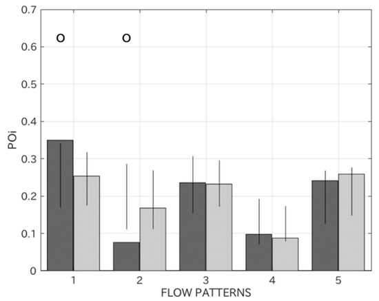
Figure 4.
Bar chart for POi for the PRE (dark shades) and POST (light shades) periods. Error bars indicate 95% intervals obtained using the bootstrap method. Circles mean that the POi value exceeds the 95% interval.
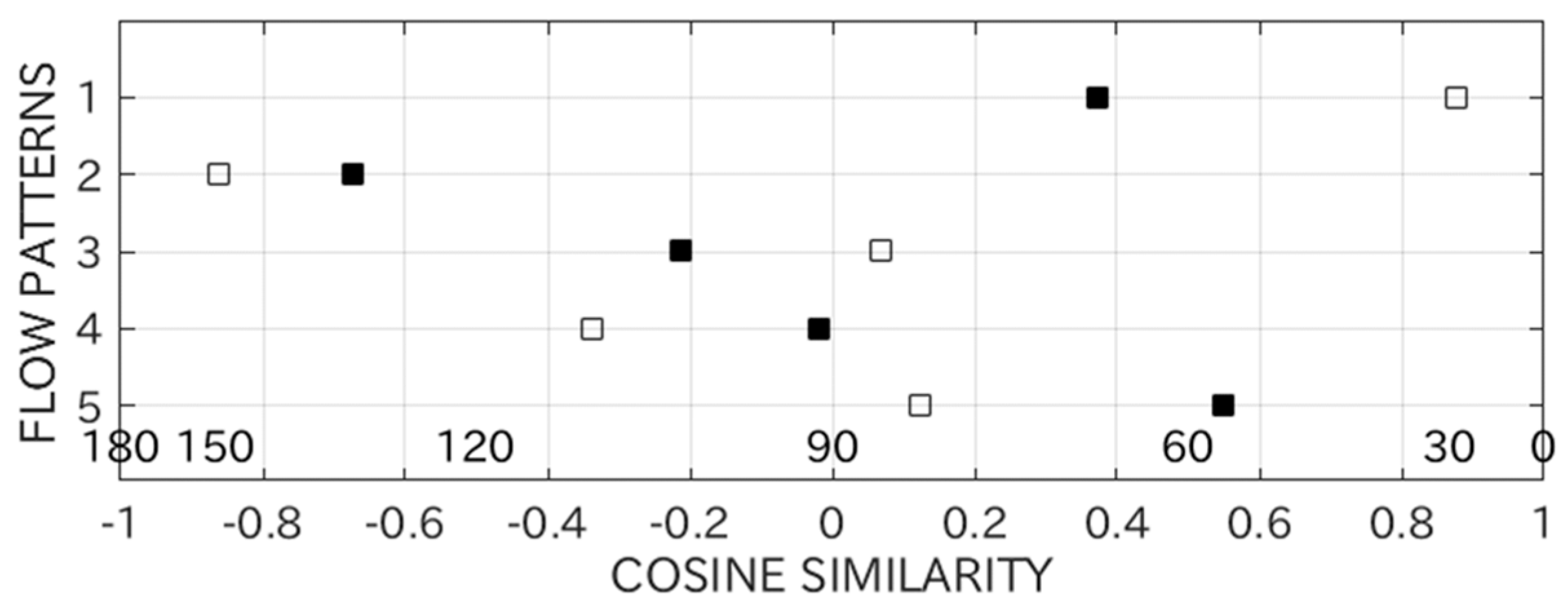
The changes in PO1 and PO2 can be understood by examining how the spatial patterns of FP1 and FP2 are related to the PRE Z500a composite. Figure 5 plots the cosine similarity between each flow pattern (Figure 1) and the PRE or POST composite map (Figure 3) of Z500a over the EA region. It is notable that FP1 is close to the PRE composite. This implies that FP1, which strengthens the planetary waves through its constructive interference with the climatological pattern, especially the EA trough (Figure 1a,f), sometimes occurs in the PRE period and contributes to the PRE composite at least in part. In contrast, FP2 is in the opposite direction to the PRE composite as expected, since the PRE composite pattern strengthens the climatological wave pattern (Figure 3a). These features are consistent with the increased PO1 and the decreased PO2 for the PRE period (Figure 4).
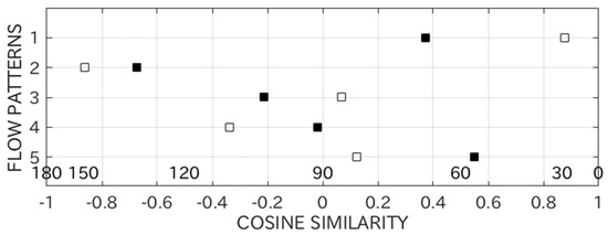
Figure 5.
Cosine similarity between each FPi pattern and the PRE or POST composite of Z500a. Unfilled markers represent PRE and filled markers POST. Several angles from 0° to 180° are also shown for reference.
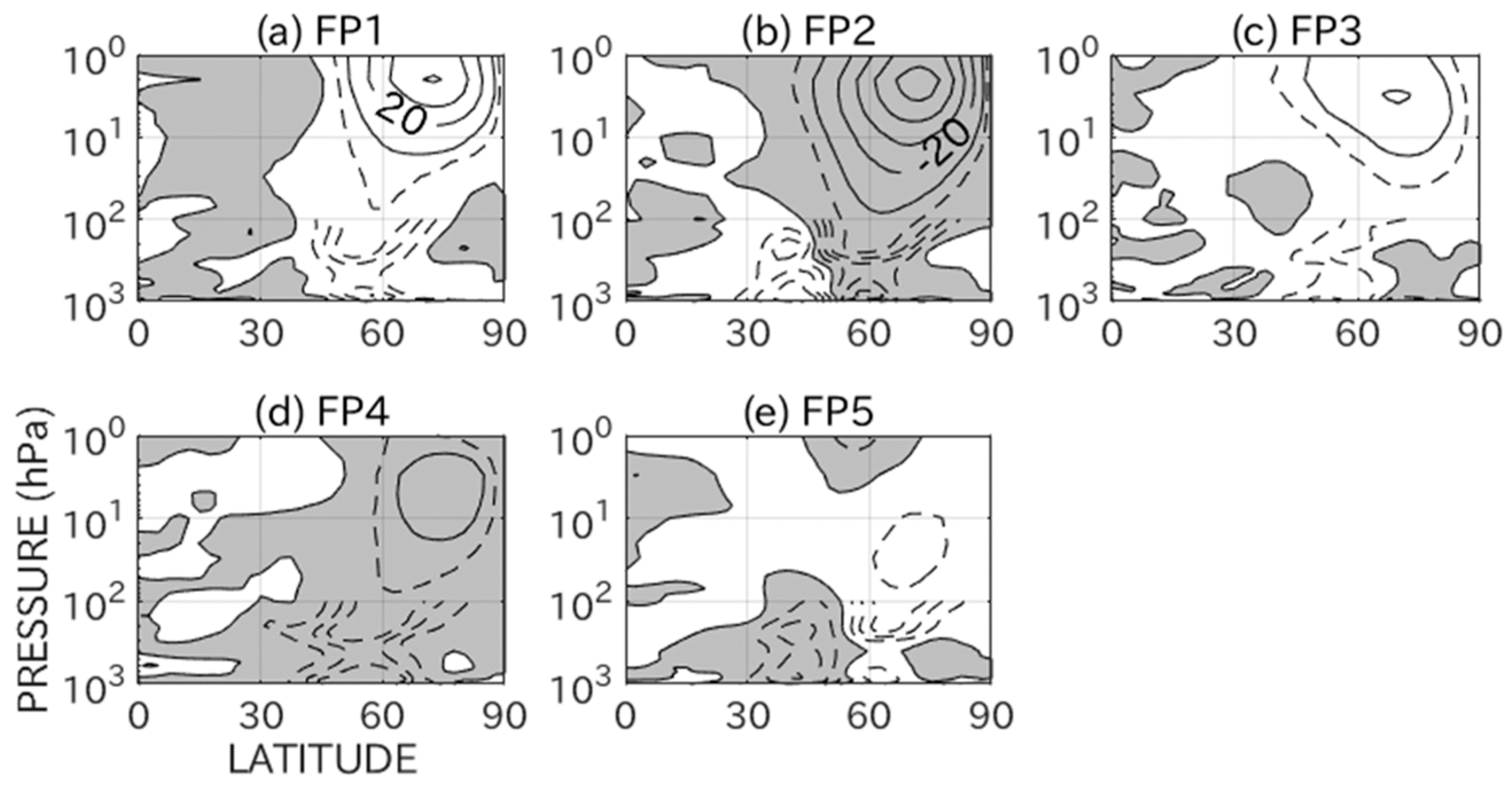
A more direct examination of HFa in combination with the occurrence of each FPi further indicates that it is larger for FP1 than usual in the extratropical troposphere and stratosphere (Figure 6a). In contrast, FP2 has predominantly negative HFa, except for lower latitudes in the troposphere (Figure 6b), consistent with Figure 1b,g. The result for FP2 is consistent with the fact that FP2 is referred to as Western Pacific [33], which is shown to induce the cooling of the Arctic stratosphere [30]. The other flow patterns have smaller HFa values in magnitude than FP1 and FP2.
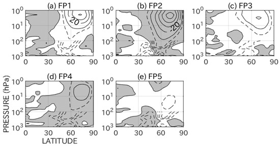
Figure 6.
HFa (K m/s) averaged over the DJF days for the five flow patterns (a–e) as indicated. Interval for solid contours is 10 K m/s. Broken contours are drawn at ±1, ±2, and ±3 below 100 hPa, in addition to ±5 K m/s. Negative values are shaded.
Since the connection between the flow patterns and MSSWs may depend on preceding anomalies over the EA region, we classify all 26 MSSWs into five subsets according to the dominant flow pattern in the PRE period for each MSSW. The dominant flow pattern is the one with the largest number of occurrence days in the PRE period (counting DJF days only). If multiple patterns have the same number of occurrence days, we prioritize the pattern of the smaller (or smallest) climatological occurrence probability. The five FP1–FP5 subsets have sample sizes of 10, 2, 6, 2, and 6, respectively.
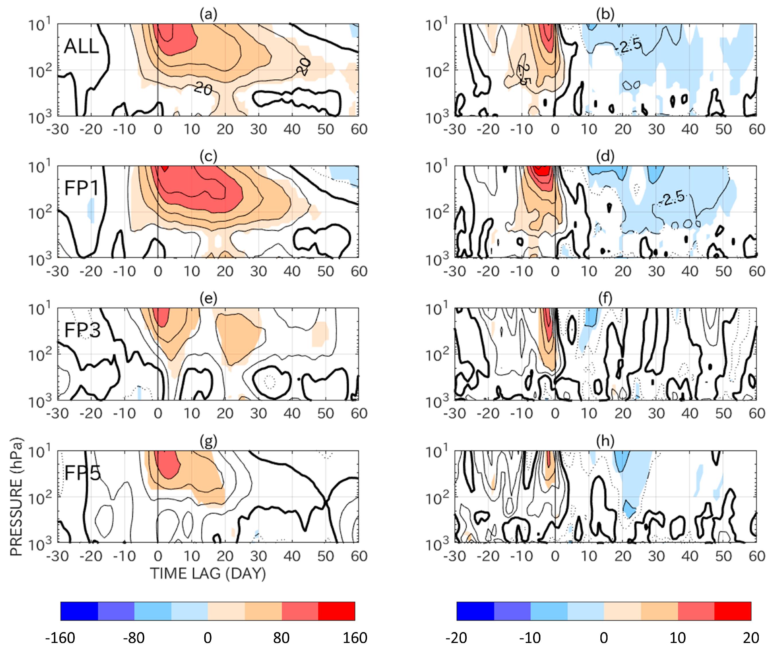
Figure 7a,b plot time–height sections of extratropical Za (zonal mean) and HFa composited with respect to the MSSW central date using all the MSSWs. The figures confirm the downward propagation of Za after the occurrence of the MSSWs, preceded by an increase in HFa (see also Figure 2). The positive Za values in the troposphere are judged to be statistically significant at the 95% confidence level (two-sided t-test), limited only around lag = +20 days (and 60 days). This limitation is probably due to the case-to-case variations combined with the limited number of MSSWs. The increase in HFa is also significant in the troposphere around lag = −7 days.

Figure 7.
(Left column) Time–height sections of Za (averaged poleward of 65°N with area weighting, further weighted with the square root of pressure/1000) composited with respect to the MSSW central date. Panel (a) uses all MSSWs, whereas the rest use (c,e,g) subsets, as indicated. For example, panel (c) uses a subset of MSSWs for which the dominant flow pattern is FP1. The contour interval is 20 m. Color shades denote values of statistical significance at the 95% level according to the two-sided t-test. Panels in the right column (b,d,f,h) are similar, but for HFa (averaged between 45–75° N, further weighted with the square root of pressure/1000). Contour interval is 2.5 K m/s.
Similar composites are obtained using a subset of the MSSWs for which the PRE dominant flow pattern is FP1 (Figure 7c,d). The composite results for this subset are basically similar to those for all MSSWs. Notably, the subset has stronger and longer-persisting Za in the lower stratosphere around lag = 0 to +40 days and stronger HFa in the stratosphere just before lag = 0 days. When two different subsets for FP3 and FP5 are further used, the composite results exhibit different features, i.e., a lack of significance for the tropospheric signals of Za and HFa. Composites are not shown for the FP2 and FP4 subsets due to their small sample sizes. These results suggest that the FP1 subset, with the largest sample size, contributes to the canonical composite picture, although the results for the FP3 and FP5 subsets may reflect the smaller sample sizes than the FP1 subset. The results also suggest the possible importance of the preceding tropospheric wave forcing [20,21] and/or lower stratospheric anomalies [18,19] for the downward propagation feature of the FP1 subset.
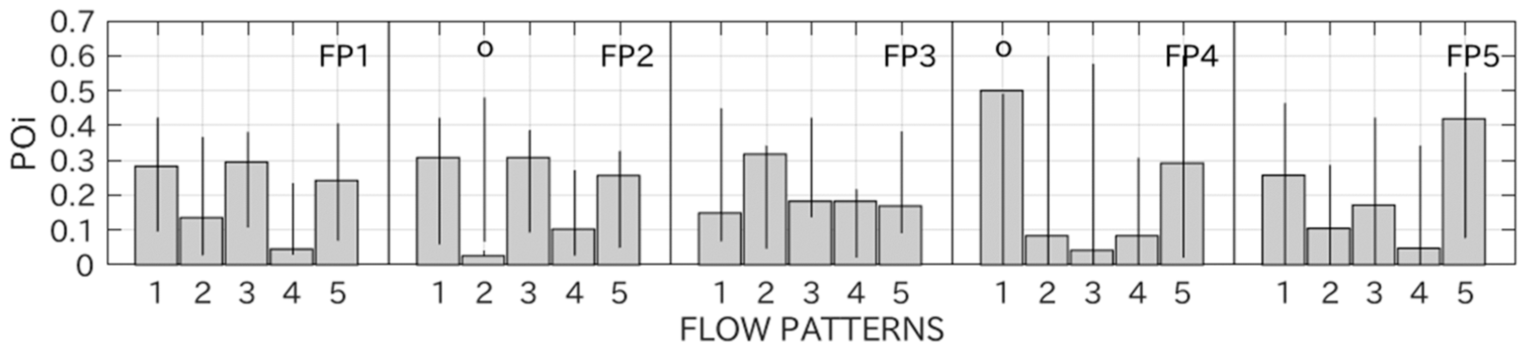
The results of POi in the POST period for each subset are shown in Figure 8. Significant changes in POi are limited when the MSSWs are classified. For example, when the dominant flow pattern is FP1, all POi values for the POST period are in 95% intervals. The MSSWs following FP2 and FP4 exhibit significant changes, but they may reflect the small sample sizes.
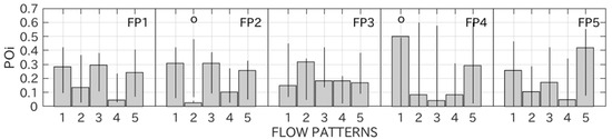
Figure 8.
Same as Figure 4, but for the POST period only, when classifying all MSSWs according to the dominant flow pattern in the PRE period. The dominant pattern is denoted in each panel as FPi.
4. Summary and Discussion
This study investigated the possible connection between winter EA flow patterns in the troposphere and anomalous SPV states using a reanalysis dataset. Five flow patterns were identified in our analysis procedures, similar to previous studies [25,26,27,33], and reasonably reproduced the results from one [33] of them. Anomalous SPV states were considered in terms of MSSW occurrence. A motivation for this study is that a possible connection between the stratosphere and troposphere, especially downward coupling, remains relatively unexplored for the Pacific region, including the EA, in comparison to the North Atlantic and Eurasia regions. The regime perspective may be useful to explore the connection.
The most notable connection found in this study is that PO1 for the PRE period is higher than usual, whereas PO2 is conversely lower. These changes can be understood in terms of their interference with the climatological tropospheric planetary wave pattern. By constructively interfering, especially with the EA trough, FP1 strengthens the planetary wave activity (HF) in the extratropical troposphere and stratosphere; such strengthening is likely to sometimes occur in the PRE period and contribute to the PRE Z500a composite, at least in part. FP2 is in the opposite sense (destructive interference) and is unlikely to occur in the PRE period. This is consistent with the reference of FP2 as the Western Pacific pattern [30,33]. Connections in the other conditions, such as changes for the POST period, are relatively unclear. Notably, a subset of MSSWs led by FP1 reproduces the canonical MSSW composite picture, including positive Za at high latitudes in the troposphere after the MSSWs, whereas such reproducibility is weak or absent in the other subsets.
Combined with previous studies, this study suggests that the connection between the stratosphere and troposphere, when viewed from a regional regime perspective, may differ among different regions. In the EA region of interest in this study, upward coupling, i.e., flow patterns affecting the wave activity flux in the troposphere and stratosphere, is notable, whereas stratospheric downward influence is relatively unclear. On the other hand, around the North Atlantic, the downward coupling, i.e., stratospheric influence on regimes relevant to the NAM or NAO, is clear [25,26,27], consistent with the composite picture of MSSWs [2]. The upward coupling in the EA region and the downward coupling in the North Atlantic region may further suggest an interregional connection through the SPV. This connection seems analogous, e.g., to the idea that an El Niño sea surface temperature condition leads to a weakening of the SPV by strengthening the planetary wave pattern via the Pacific–North America pattern; the weakened SPV in turn exerts a downward influence on the troposphere, i.e., it tends to induce the negative phase of the NAM or NAO [37,38,39].
Regarding the EA flow patterns, the relatively unclear downward coupling may be constrained by the key index for the SPV, i.e., MSSW occurrence, which is based on the zonal mean. The analysis leaves the possibility of downward coupling around the EA region when considering zonally varying or regional anomalies of the SPV [32,40]. Furthermore, the EA flow patterns examined here have shorter persistent periods around a couple of days than those around the North Atlantic. In particular, at least some of the EA flow patterns represent migrating low-pressure systems [33]. A clearer downward coupling may be demonstrated considering different and/or more persistent regimes over/around the EA region.
It will be useful to extend regime-based analyses such as the present one to climate simulation and subseasonal-to-seasonal forecast data. One could first examine the reproducibility of the climate simulation and the skill of the forecast data in terms of the connection between weather regimes and SPV anomalies. If the reproducibility is confirmed, one could further use such numerical simulation data to increase the sample size, especially for MSSWs [41,42]. Finally, whereas a statistical analysis may not prove causality between weather regimes and SPV anomalies, well-designed numerical experiments could contribute to such proof. Investigation in this direction will be conducted for the two MSSWs in 2018 and 2019 in the framework of the SNAPSI project [43] and be reported elsewhere.
Funding
This study was partly supported by JSPS Grant-in-Aid for Scientific Research (C) 22K03719.
Institutional Review Board Statement
Not applicable.
Informed Consent Statement
Not applicable.
Data Availability Statement
The JRA-55 data were made available by the Japan Meteorological Agency. The JRA-55 data were obtained from the Research Data Archive at the National Center for Atmospheric Research, Computational and Information Systems Laboratory at https://doi.org/10.5065/D6HH6H41.
Conflicts of Interest
The author declares no conflicts of interest.
References
- Butchart, N. The Stratosphere: A Review of the Dynamics and Variability. Weather. Clim. Dyn. 2022, 3, 1237–1272. [Google Scholar] [CrossRef]
- Kidston, J.; Scaife, A.A.; Hardiman, S.C.; Mitchell, D.M.; Butchart, N.; Baldwin, M.P.; Gray, L.J. Stratospheric Influence on Tropospheric Jet Streams, Storm Tracks and Surface Weather. Nat. Geosci. 2015, 8, 433–440. [Google Scholar] [CrossRef]
- Baldwin, M.P.; Ayarzagüena, B.; Birner, T.; Butchart, N.; Butler, A.H.; Charlton-Perez, A.J.; Domeisen, D.I.V.; Garfinkel, C.I.; Garny, H.; Gerber, E.P.; et al. Sudden Stratospheric Warmings. Rev. Geophys. 2021, 59, e2020RG000708. [Google Scholar] [CrossRef]
- Matsuno, T. Vertical Propagation of Stationary Planetary Waves in the Winter Northern Hemisphere. J. Atmos. Sci. 1970, 27, 871–883. [Google Scholar] [CrossRef]
- Matsuno, T. A Dynamical Model of the Stratospheric Sudden Warming. J. Atmos. Sci. 1971, 28, 1479–1494. [Google Scholar] [CrossRef]
- Limpasuvan, V.; Thompson, D.W.J.; Hartmann, D.L. The Life Cycle of the Northern Hemisphere Sudden Stratospheric Warmings. J. Clim. 2004, 17, 2584–2596. [Google Scholar] [CrossRef]
- Polvani, L.M.; Waugh, D.W. Upward Wave Activity Flux as a Precursor to Extreme Stratospheric Events and Subsequent Anomalous Surface Weather Regimes. J. Clim. 2004, 17, 3548–3554. [Google Scholar] [CrossRef]
- Martius, O.; Polvani, L.M.; Davies, H.C. Blocking Precursors to Stratospheric Sudden Warming Events. Geophys. Res. Lett. 2009, 36, L14806. [Google Scholar] [CrossRef]
- Garfinkel, C.I.; Hartmann, D.L.; Sassi, F. Tropospheric Precursors of Anomalous Northern Hemisphere Stratospheric Polar Vortices. J. Clim. 2010, 23, 3282–3299. [Google Scholar] [CrossRef]
- Nishii, K.; Nakamura, H.; Orsolini, Y.J. Geographical Dependence Observed in Blocking High Influence on the Stratospheric Variability through Enhancement and Suppression of Upward Planetary-Wave Propagation. J. Clim. 2011, 24, 6408–6423. [Google Scholar] [CrossRef]
- Bao, M.; Tan, X.; Hartmann, D.L.; Ceppi, P. Classifying the Tropospheric Precursor Patterns of Sudden Stratospheric Warmings. Geophys. Res. Lett. 2017, 44, 8011–8016. [Google Scholar] [CrossRef]
- Scaife, A.A.; Folland, C.K.; Alexander, L.V.; Moberg, A.; Knight, J.R. European Climate Extremes and the North Atlantic Oscillation. J. Clim. 2008, 21, 72–83. [Google Scholar] [CrossRef]
- Kolstad, E.W.; Breiteig, T.; Scaife, A.A. The Association between Stratospheric Weak Polar Vortex Events and Cold Air Outbreaks in the Northern Hemisphere. Q. J. R. Meteorol. Soc. 2010, 136, 886–893. [Google Scholar] [CrossRef]
- King, A.D.; Butler, A.H.; Jucker, M.; Earl, N.O.; Rudeva, I. Observed Relationships Between Sudden Stratospheric Warmings and European Climate Extremes. J. Geophys. Res. Atmos. 2019, 124, 13943–13961. [Google Scholar] [CrossRef]
- Domeisen, D.I.V.; Butler, A.H. Stratospheric Drivers of Extreme Events at the Earth’s Surface. Commun. Earth Environ. 2020, 1, 59. [Google Scholar] [CrossRef]
- Kolstad, E.W. Higher Ocean Wind Speeds during Marine Cold Air Outbreaks. Q. J. R. Meteorol. Soc. 2017, 143, 2084–2092. [Google Scholar] [CrossRef]
- Baldwin, M.P.; Dunkerton, T.J. Propagation of the Arctic Oscillation from the Stratosphere to the Troposphere. J. Geophys. Res. Atmos. 1999, 104, 30937–30946. [Google Scholar] [CrossRef]
- Hitchcock, P.; Shepherd, T.G.; Taguchi, M.; Yoden, S.; Noguchi, S. Lower-Stratospheric Radiative Damping and Polar-Night Jet Oscillation Events. J. Atmos. Sci. 2013, 70, 1391–1408. [Google Scholar] [CrossRef]
- Runde, T.; Dameris, M.; Garny, H.; Kinnison, D.E. Classification of Stratospheric Extreme Events According to Their Downward Propagation to the Troposphere. Geophys. Res. Lett. 2016, 43, 6665–6672. [Google Scholar] [CrossRef]
- Nakagawa, K.I.; Yamazaki, K. What Kind of Stratospheric Sudden Warming Propagates to the Troposphere? Geophys. Res. Lett. 2006, 33, L04801. [Google Scholar] [CrossRef]
- Karpechko, A.Y.; Hitchcock, P.; Peters, D.H.W.; Schneidereit, A. Predictability of Downward Propagation of Major Sudden Stratospheric Warmings. Q. J. R. Meteorol. Soc. 2017, 143, 1459–1470. [Google Scholar] [CrossRef]
- Dai, Y.; Hitchcock, P. Understanding the Basin Asymmetry in Surface Response to Sudden Stratospheric Warmings from an Ocean–Atmosphere Coupled Perspective. J. Clim. 2021, 34, 8683–8698. [Google Scholar] [CrossRef]
- Scaife, A.A.; Baldwin, M.P.; Butler, A.H.; Charlton-Perez, A.J.; Domeisen, D.I.V.; Garfinkel, C.I.; Hardiman, S.C.; Haynes, P.; Karpechko, A.Y.; Lim, E.P.; et al. Long-Range Prediction and the Stratosphere. Atmos. Chem. Phys. 2022, 22, 2601–2623. [Google Scholar] [CrossRef]
- Hannachi, A.; Straus, D.M.; Franzke, C.L.E.; Corti, S.; Woollings, T. Low-Frequency Nonlinearity and Regime Behavior in the Northern Hemisphere Extratropical Atmosphere. Rev. Geophys. 2017, 55, 199–234. [Google Scholar] [CrossRef]
- Charlton-Perez, A.J.; Ferranti, L.; Lee, R.W. The Influence of the Stratospheric State on North Atlantic Weather Regimes. Q. J. R. Meteorol. Soc. 2018, 144, 1140–1151. [Google Scholar] [CrossRef]
- Domeisen, D.I.V.; Grams, C.M.; Papritz, L. The Role of North Atlantic-European Weather Regimes in the Surface Impact of Sudden Stratospheric Warming Events. Weather. Clim. Dyn. 2020, 1, 373–388. [Google Scholar] [CrossRef]
- Lee, S.H.; Furtado, J.C.; Charlton-Perez, A.J. Wintertime North American Weather Regimes and the Arctic Stratospheric Polar Vortex. Geophys. Res. Lett. 2019, 46, 14892–14900. [Google Scholar] [CrossRef]
- Greatbatch, R.J.; Gollan, G.; Jung, T.; Kunz, T. Factors Influencing Northern Hemisphere Winter Mean Atmospheric Circulation Anomalies during the Period 1960/61 to 2001/02. Q. J. R. Meteorol. Soc. 2012, 138, 1970–1982. [Google Scholar] [CrossRef]
- Butler, A.H.; Sjoberg, J.P.; Seidel, D.J.; Rosenlof, K.H. A Sudden Stratospheric Warming Compendium. Earth Syst. Sci. Data 2017, 9, 63–76. [Google Scholar] [CrossRef]
- Nishii, K.; Nakamura, H.; Orsolini, Y.J. Cooling of the Wintertime Arctic Stratosphere Induced by the Western Pacific Teleconnection Pattern. Geophys. Res. Lett. 2010, 37, L13805. [Google Scholar] [CrossRef]
- Jeong, J.H.; Kim, B.M.; Ho, C.H.; Chen, D.; Lim, G.H. Stratospheric Origin of Cold Surge Occurrence in East Asia. Geophys. Res. Lett. 2006, 33, L14710. [Google Scholar] [CrossRef]
- Zhang, Y.; Si, D.; Ding, Y.; Jiang, D.; Li, Q.; Wang, G. Influence of Major Stratospheric Sudden Warming on the Unprecedented Cold Wave in East Asia in January 2021. Adv. Atmos. Sci. 2022, 39, 576–590. [Google Scholar] [CrossRef]
- Matsueda, M.; Kyouda, M. Wintertime East Asian Flow Patterns and Their Predictability on Medium-Range Timescales. Sci. Online Lett. Atmos. 2016, 12, 121–126. [Google Scholar] [CrossRef]
- Kobayashi, S.; Ota, Y.; Harada, Y.; Ebita, A.; Moriya, M.; Onoda, H.; Onogi, K.; Kamahori, H.; Kobayashi, C.; Endo, H.; et al. The JRA-55 Reanalysis: General Specifications and Basic Characteristics. J. Meteorol. Soc. Japan Ser. II 2015, 93, 5–48. [Google Scholar] [CrossRef]
- Charlton, A.J.; Polvani, L.M. A New Look at Stratospheric Sudden Warmings. Part I: Climatology and Modeling Benchmarks. J. Clim. 2007, 20, 449–469. [Google Scholar] [CrossRef]
- Baldwin, M.P.; Dunkerton, T.J. Stratospheric Harbingers of Anomalous Weather Regimes. Science (1979) 2001, 294, 581–584. [Google Scholar] [CrossRef] [PubMed]
- Ineson, S.; Scaife, A.A. The Role of the Stratosphere in the European Climate Response to El Nĩo. Nat. Geosci. 2009, 2, 32–36. [Google Scholar] [CrossRef]
- Polvani, L.M.; Sun, L.; Butler, A.H.; Richter, J.H.; Deser, C. Distinguishing Stratospheric Sudden Warmings from ENSO as Key Drivers of Wintertime Climate Variability over the North Atlantic and Eurasia. J. Clim. 2017, 30, 1959–1969. [Google Scholar] [CrossRef]
- Domeisen, D.I.V.; Garfinkel, C.I.; Butler, A.H. The Teleconnection of El Niño Southern Oscillation to the Stratosphere. Rev. Geophys. 2019, 57, 5–47. [Google Scholar] [CrossRef]
- Kretschmer, M.; Cohen, J.; Matthias, V.; Runge, J.; Coumou, D. The Different Stratospheric Influence on Cold-Extremes in Eurasia and North America. NPJ Clim. Atmos. Sci. 2018, 1, 44. [Google Scholar] [CrossRef]
- Spaeth, J.; Birner, T. Stratospheric Modulation of Arctic Oscillation Extremes as Represented by Extended-Range Ensemble Forecasts. Weather. Clim. Dyn. 2022, 3, 883–903. [Google Scholar] [CrossRef]
- Bett, P.E.; Scaife, A.A.; Hardiman, S.C.; Thornton, H.E.; Shen, X.; Wang, L.; Pang, B. Using Large Ensembles to Quantify the Impact of Sudden Stratospheric Warmings and Their Precursors on the North Atlantic Oscillation. Weather. Clim. Dyn. 2023, 4, 213–228. [Google Scholar] [CrossRef]
- Hitchcock, P.; Butler, A.; Charlton-Perez, A.; Garfinkel, C.I.; Stockdale, T.; Anstey, J.; Mitchell, D.; Domeisen, D.I.V.; Wu, T.; Lu, Y.; et al. Stratospheric Nudging And Predictable Surface Impacts (SNAPSI): A Protocol for Investigating the Role of Stratospheric Polar Vortex Disturbances in Subseasonal to Seasonal Forecasts. Geosci. Model. Dev. 2022, 15, 5073–5092. [Google Scholar] [CrossRef]


Disclaimer/Publisher’s Note: The statements, opinions and data contained in all publications are solely those of the individual author(s) and contributor(s) and not of MDPI and/or the editor(s). MDPI and/or the editor(s) disclaim responsibility for any injury to people or property resulting from any ideas, methods, instructions or products referred to in the content. |
© 2024 by the author. Licensee MDPI, Basel, Switzerland. This article is an open access article distributed under the terms and conditions of the Creative Commons Attribution (CC BY) license (https://creativecommons.org/licenses/by/4.0/).