Abstract
Existing sub-grid parameterization schemes for clear-sky direct solar radiation (SPS-CSDSR) assume that the sub-grid cells have the same atmospheric transparency. This study shows that in undulating terrain, significant errors can occur when the sub-grid is in turbid weather or partly above the cloud top. A correction factor was proposed. It can effectively eliminate errors under a cloudless sky and can reduce some errors when part of the sub-grid is above the cloud or fog top. For atmospheric models with high horizontal resolution, example test verification shows that the cast shadowless coverage method can lead to large errors. It should no longer be used based on current computing power. These improvements and the high-precision fast terrain occlusion algorithm in Part I will allow SPS-CSDSR to achieve unprecedented high accuracy. Based on the proposed daily interpolation method, the high-precision SPS-CSDSR is also feasible for regional climate simulation. The analysis pointed out that the sub-grid terrain radiative effect (STRE) is distributed over inclined surfaces with larger areas and at different heights. Existing methods of coupling STRE on one flat surface have certain physical drawbacks. This paper suggests introducing parameterization of STRE at different altitudes and improving the coupling of land–air.
1. Introduction
This paper is Part II of the study. The variable symbols from Part I [1] will continue to be used.
As for SPS-CSSDSI, after high-resolution Digital Elevation Model (DEM) data has been widely used, many scholars have proposed approximate methods to reduce computation and advance research in this field [2,3,4,5,6,7,8,9,10]. These approximate methods mainly include: (1) ignoring cast shadows, reducing DEM data resolution, using small terrain occlusion search radius, and terrain occlusion processing with reduced accuracy, etc.; (2) assuming the same atmospheric transparency for sub-grid cells, using the same direct normal irradiance (DNI) in sub-grid cells. (3) In order to use the solar position (solar altitude and azimuth angle) of an atmospheric model, parameterized CSHDSI without cast shadows is calculated first, and then the cast shadowless coverage is used to correct. This method is referred to as the cast shadowless coverage method in this paper.
Part I of this study proposes a high-precision, fast terrain occlusion algorithm (HPFTOA) [1]. It uses a lossless, fast search radius and other methods to speed up computation and takes into account the curvature of the earth. The verification analysis shows that the HPFTOA can carry out large-scale computations based on the DEM data with a resolution of 90 m (DEM90). For a region with extremely complex terrain such as the eastern Tibetan Plateau, with a size of 80° × 60° and a calculation time interval of 30 min, using 300 cores of CPU Gold 6526Y, the wall clock times are 44.8 and 50.9 min during the daytime in the winter solstice and the summer solstice, respectively. This computation cost is feasible for the regional weather simulation over several days. It means the SPS-CSDSR should no longer use the previous approximation algorithms (Table 1 in Part I [1]) to process cast shadows. The situation in which the past SPS-CSSDSI was severely restricted by terrain occlusion calculations will fundamentally change.
The actual atmospheric transparency usually increases with altitude in a cloudless sky, as does DNI. In mountainous regions, it often appears that the higher part of the mountain is above clouds or fog. However, the existing SPS-CSDSRs [2,3,4,5,6,7,8,9,10] are all based on assuming the same atmospheric transparency for sub-grid cells. Equation (4) in Part I [1] also follows this assumption, which may lead to errors. Section 2 analyzes this issue and provides an improvement plan. This improvement and the HPFTOA will constitute the high-precision SPS-CSDSR.
In this paper, the necessary pre-research for the application of the high-precision SPS-CSDSR based on the DEM90 and the HPFOTA is conducted. This includes determining whether to utilize the cast shadowless coverage method, how to further reduce computational costs, and correctly coupling STRE into the atmospheric model.
The cast shadowless coverage method has been developed in recent years [10], which is the most mature SPS-CSDSR before this study. It does not ignore cast shadows and uses DEM90. However, it has not been sufficiently validated. A validation will be performed in Section 3.
Although the HPFTOA can be used with guaranteed accuracy, it still has certain computational costs. Developing a more economical method will enhance its application. For this, the feasibility of calculating the STRE factor by day interpolation will be researched in Section 4.
In mountainous regions, the actual physical mechanism of the STRE is that the radiation is dispersed across the inclined surfaces of a larger area at different heights. However, existing land surface physical models are designed for flat land, utilizing real physical parameters such as aerodynamic roughness, emissivity of the surface, heat capacity of the soil, etc. Past research work (such as [6,7,8,9,11,12,13,14]) coupled parameterized STRE with the land surface in atmospheric models. For direct solar radiation, when coupling the terrain effect factor , the downward direct solar radiation flux is instead by at the land surface in atmospheric model. is calculated by the atmospheric model without terrain. is the solar zenith angle. This has certain physical drawbacks. Section 5 analyzes this problem.
The last part of Section 6 summarized this study’s work.
2. Considering Atmospheric Transparency Differences in Sub-Grid
The actual atmospheric transparency increases with altitude, as does DNI. At times, a part of the sub-grid can be above the cloud tops. All existing SPS-CSDSRs are designed based on assuming the same atmospheric transparency for sub-grid cells, which may lead to errors.
There are two scenarios: the sub-grid under a cloudless sky; part of the sub-grid above the cloud or fog top.
2.1. The Sub-Grid under a Cloudless Sky
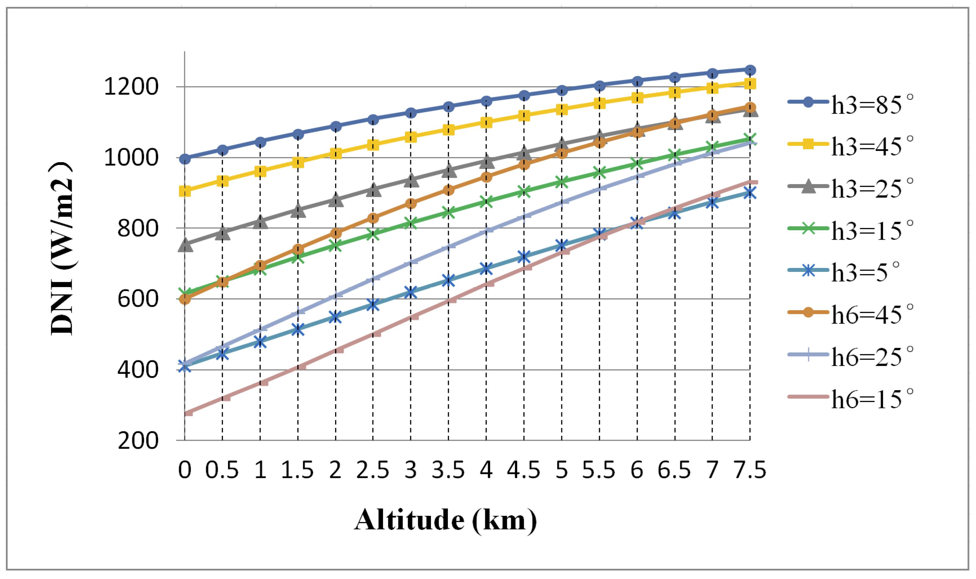
The DNI model in Part I was used to make Figure 1. It shows a set of curves of DNI with different solar altitude angles when the sub-grid is under a cloudless sky. Upon observing Figure 1, it is evident that the DNI increases in an approximately linear fashion with altitude. Then,
where and indicate the atmospheric model grid cell and the sub-grid cell, respectively. is the sequence number of a sub-grid cell. is the altitude. is the vertical change rate of . and can be obtained from the radiation model of the atmospheric model.
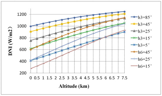
Figure 1.
The curves of DNI with altitude. h stands for solar altitude angle. 3 and 6 stand that are 3.0 and 6.0, respectively.
From Figure 1, is positive. So the DNI has a negative deviation above and a positive deviation below .
Equation (4) in Part I [1] can be changed as follows:
with
where is the clear-sky horizontal direct solar irradiance. indicates parameterization. is the sunlight incidence angle between the plane normal of sub-grid cell and the solar beam. and are the surface area and the horizontal projected area of the sub-grid cell, respectively.
Equation (2) has one more term than Equation (4) in Part I [1]. Usually, is the mean value of altitude at sub-grid cell, and then () is the altitude anomaly at a sub-grid cell. Then, can be referred to as the sub-grid altitude anomaly correction term for Equation (4) in Part I [1].
The calculation of Equations (2) and (3) can be divided into offline steps (before the atmospheric model runs) and online steps (while the atmospheric model running).
Offline steps:
Online steps:
In the atmospheric model, is the altitude at the bottom level, and is the altitude meters above . can be a fixed value or adjusted based on the altitudes of sub-grid cells. and are DNI at and , respectively. is the downward direct solar radiation flux. is the solar zenith angle.
is close to 0 in three cases. (1) The terrain is not very undulating, so the height differences of the sub-grid cells are very small. (2) The negative deviation above the altitude of can cancel out the positive deviation below the height of . (3) is a very small value. These three cases are equivalent in that the sub-grid cells have the same DNI.
In low solar altitude, the cast shadows often appear at low places, and the positive deviation below the height of will be reduced. So assuming the sub-grid cells have the same DNI can lead to a negative error. Because increases with the increase in turbidity factor (Figure 1), the error will be more significant in turbid weather.
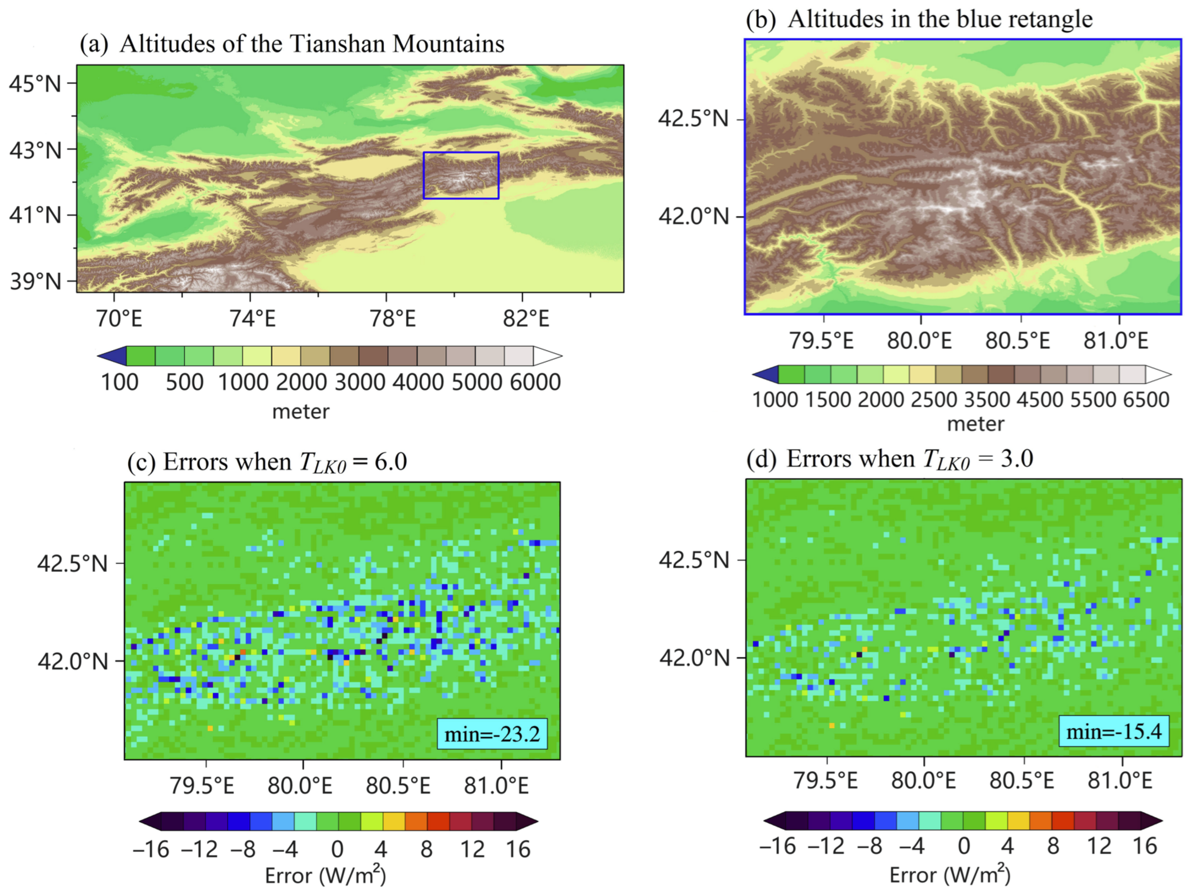
The role of was verified in the middle part of the Tianshan Mountains (Figure 2a,b). The Tianshan Mountains are adjacent to the six major deserts. Turbid weather often occurs there. The errors in by using or not using were compared in general () and turbid weather ( 6.0). This test used DEM90 [15], the HPFTOA, and 2TPA. 2TPA is an algorithm for decomposing sub-grid cells into two triangles (see Part I). Set m. The times are from 08:40 LST to 16:40 LST during the 1 h interval of the daytime on Winter Solstice 2022. The horizontal resolution is about 3 km (33 × 33 sub-grid cells in a parent grid cell).
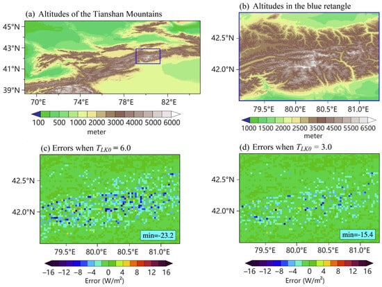
Figure 2.
The error analysis for middle part of the Tianshan Mountains. (a) Altitudes of the Tianshan Mountains; (b) altitudes of the blue rectangle in (a); (c,d) the errors in at 09:40 LST on the Winter Solstice when not using with the solar altitude angle of 12.7°. The “min” is the minimum value of errors.
The result is that when using , the maximum absolute error in is less than 2.3 W/m2 () during the daytime. When the sub-grid DNIs are the same (not using ), which mainly leads to negative discrete errors (Figure 2c,d). The maximum absolute error in can reach 23.3 W/m2 in the turbid weather () during the daytime. In general weather (), the error is small (Figure 2d).
When sub-grid is turbid, assuming that sub-grid cells have the same atmospheric transparency will lead to significant errors. For a cloudless sky, the correction factors of can effectively eliminate errors.
This also reminds us that and must meet the condition for SPS-CSDSR. Otherwise, unexpected deviations can be brought about. Therefore, it is necessary to unify the altitude data sources of the atmospheric model and SPS-CSDSR.
2.2. A Part of the Sub-Grid Is above the Cloud Top
In this case, the lower part of the mountain is obscured by low clouds or fog, and the higher part of the mountain can receive direct solar radiation. This situation is often seen, such as the sea of clouds or fog at the bottom of the mountain. Obviously, assuming the same DNI in the sub-grid will lead to a large error at this time. The size of the error is related to the coverage of clouds or fogs.
At this time, can play a certain role in correction. For example, when more than 80% of the sub-grid is above the top of the fogs, , and CSHDSI is evenly distributed in sub-grids, assuming the same DNI in each sub-grid will lead to a negative deviation of 80%. When using , the error can be reduced to 30%. But this accuracy may still not be enough.
In theory, this physical phenomenon can only be correctly represented when parameterized at several levels and finally synthesized with the parameterized values of these layers. However, the implementation of this layered parameterization method will depend on the model’s forecasting performance in mountain clouds. Moreover, the height difference of the model grid cell is different from that of the sub-grid. Specific methods in this regard require thematic research based on a detailed assessment of atmospheric model cloud forecasts.
Obviously, before this layered parameterization method can be implemented, the use of is very beneficial to reduce the SPS-CSDSR error in mountainous areas with low clouds or fog. At this time, the range of recommendation is . is the mean altitude of the sub-grid cells above , and is the maximum value of the altitudes of the sub-grid cells.
2.3. Summary for This Chapter
When sub-grid is in turbid weather or partly above the cloud top, assuming that sub-grid cells have the same atmospheric transparency will lead to significant errors, and the latter errors can be more serious.
For a cloudless sky, the correction factors can effectively eliminate errors. When part of the sub-grid is above the cloud or fog top, can reduce some errors. More effective layered parameterization methods await further research based on the analysis of specific atmospheric models’ performance in forecasting mountain low clouds and fogs.
3. Example Test of a Recent SPS-CSDSR
This SPS-CSDSR is from Huang et al. [10]. It consists of Equations (6)–(14).
where is the identifier of the atmospheric model grid. , , , , and are the parameterized value of the clear-sky direct solar irradiance (CSDSI), the solar zenith angle and azimuth, grid spacing (km), the latitude, and the number of DEM90 spacing, respectively. In cast shadow ; otherwise . In this paper, for atmospheric models with a horizontal resolution of 3 km (Model-3Km), . For atmospheric models with a horizontal resolution of 9 km (Model-9Km), .
This SPS-CSDSR was based on the method of He et al. [9] and has been applied in the study works of Gu et al. [13] and Cai er al. [14]. It does not ignore the cast shadow, uses DEM90, and has an occlusion search radius of 27 km. It was the most mature SPS-CSDSR before this study.
In order to use the solar position (solar altitude and azimuth angle) of an atmospheric model, this SPS-CSDSR first parameterizes CSDSI without casting shadows, and then uses to correct it. It uses a prefabricated lookup table to determine , including 100 horizontal azimuths, 100 levels of maximum cover angle sine, and a 27 km search radius.
In order to be consistent with CSHDSI in Equation (1) in Part I [1], (Equation (15)) will be compared in this paper. It reduces the area conversion term .
According to this SPS-CSDSR [10], this test will use the third-order finite difference [16] to calculate the slope and aspect of the sub-grid cell.
Because of the high computation cost of the lookup table, the cast shadowless coverage will be calculated by Equation (11) instead of looking up a table. This is more accurate. will be obtained based on the HPFTOA with a 27 km search radius.
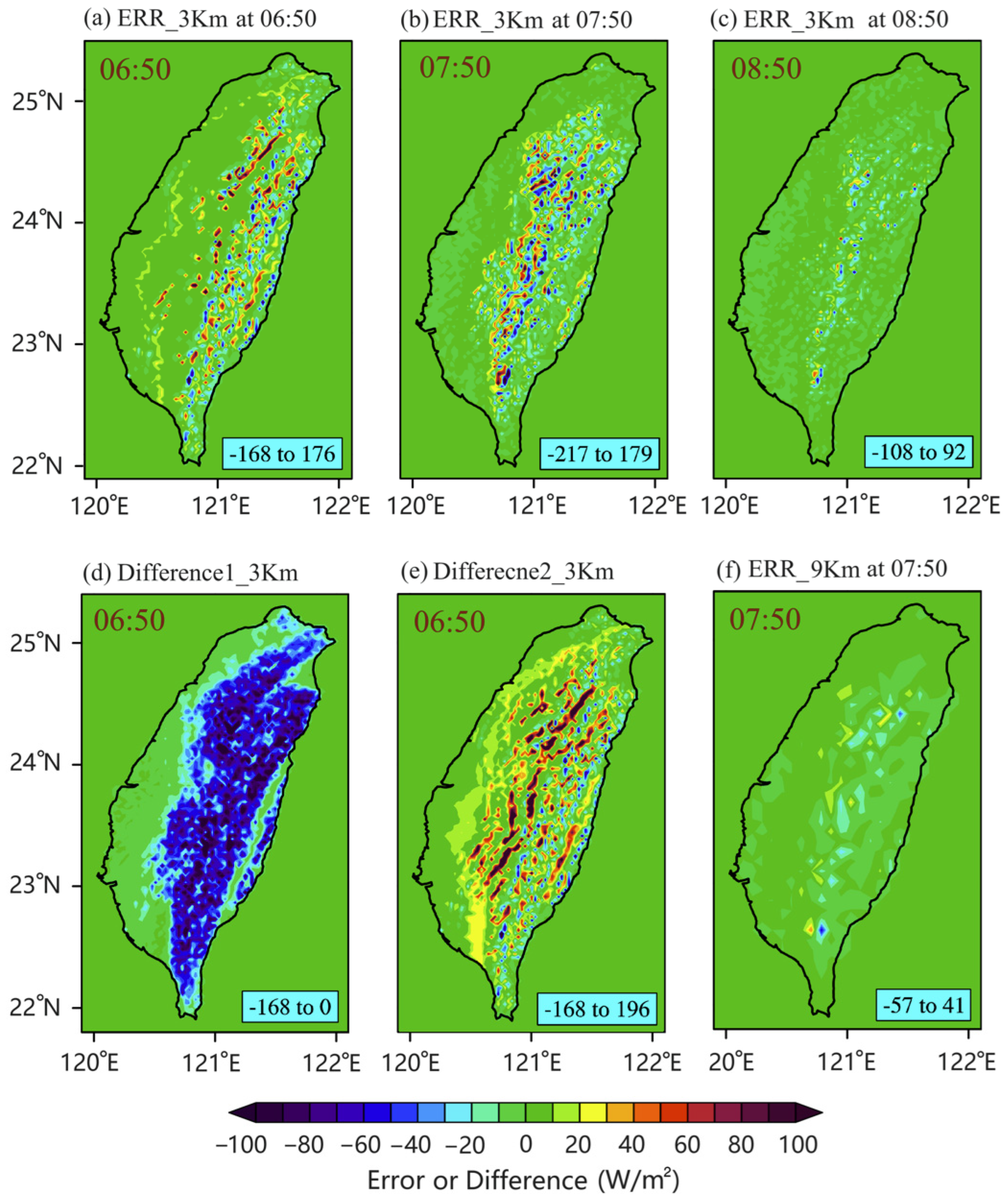
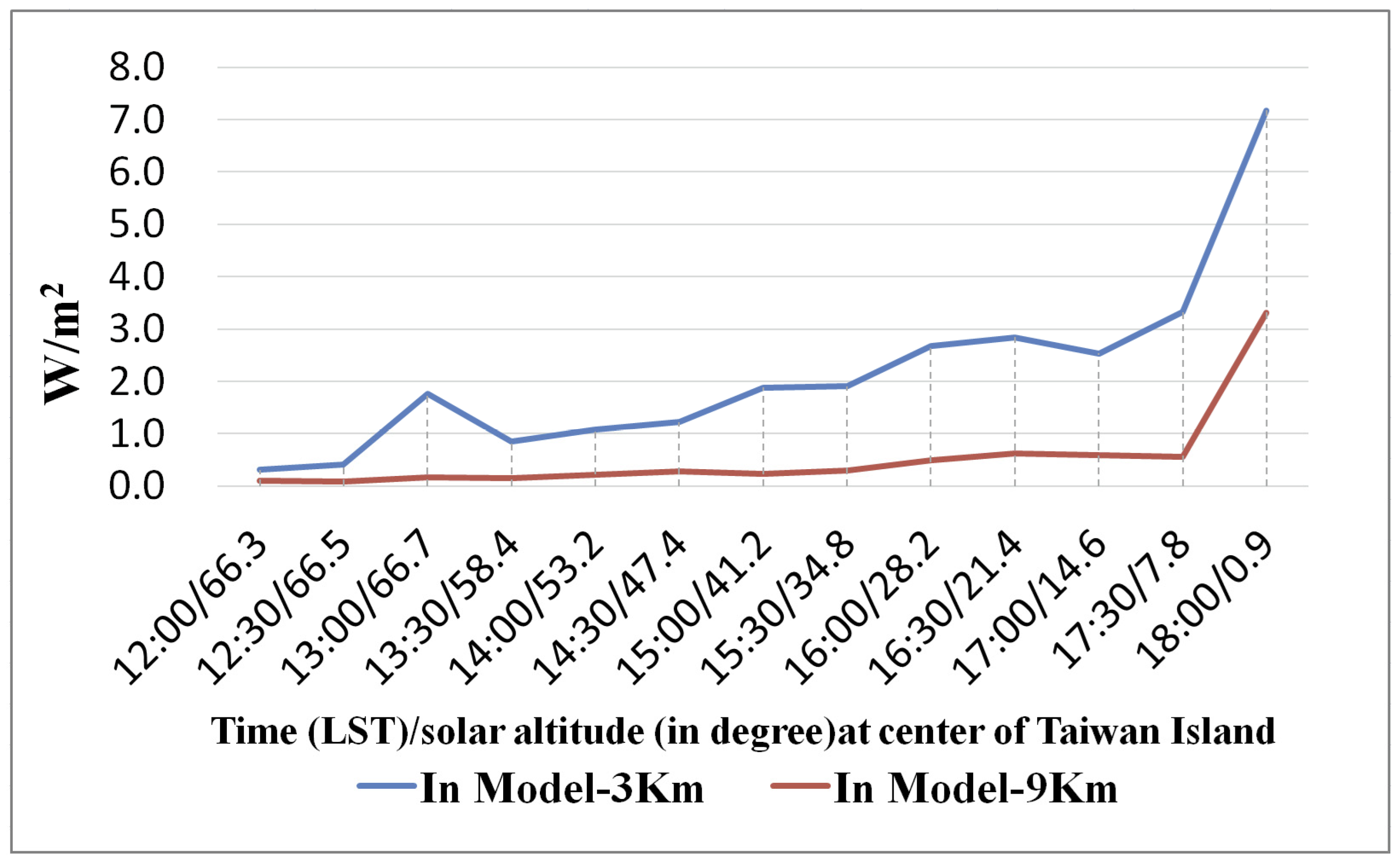
The simulation test is on Taiwan Island during the Winter Solstice 2022, taking . Taiwan Island is surrounded by the ocean, and its terrain is very complex [1]. It is suitable for verifying the radiation model for mountains. Figure 3a–c shows the errors in of Model-3Km are large at low solar altitude angles. These errors distorted the spatial distribution of STRE. Judging by the magnitude of the error, it would lead to distortions of local circulation in the atmospheric model.

Figure 3.
The errors (a–c) in of Model-3Km at 06:50, 07:50, and 08:50 on the Winter Solstice in 2022, where the solar altitude angles are 2.6, 14.4, and 25.1 degrees at the center, respectively. The blue label indicates the range of the errors. (d) The difference between parameterization cast shadows and original when both ignoring cast shadows; (e) the difference between without cast shadows and with cast shadows; (f) errors in of Model-9Km at 07:50 LST.
Equation (7) was derived from the deformation of Equation (3) in Part I [1] divided by slope cosine. However, when summing each term on the right-hand side of the changed equation, the constraint that the incidence angle cosine cannot be negative was lost in Equation (7). This resulted in some values of the self-occluded sub-grid cells participating in the calculation for . This led to negative deviations (such as shown in Figure 3d) at low solar altitude angles when the CSHDSI ignored cast shadows.
In Figure 3e, only ignored cast shadows. It shows that a lot of negative errors were enough to offset some of the cast shadow. Those strong positive deviations are because there should be a lot of cast shadows there, in fact. Their values are much larger than the results that He et al. [8] verified in a smaller region.
According to Equations (12)–(14), for Model-3Km, is approximately 0.09 on Taiwan Island, and the minimum value of is about 0.91. Therefore, can only eliminate the errors when , has little correction ability for other positive errors (such as ), and has no correction ability for negative errors. So, there is still a significant positive deviation in Figure 3a, and the negative error is almost indistinguishable from Figure 3e.
For atmospheric models with a high horizontal resolution, when there is a lot of self-occlusion and cast shadows, this method [10] will lead to very large errors. When the solar altitude angle increases, the error decreases as the shadow decreases (such as Figure 3c). These errors are significantly reduced in the Model-9Km (Figure 3f); however, they are still not negligible. Therefore, this method is not suitable for models with a horizontal resolution of less than 9 km.
The calculation process of this study shows that the computation speed of Fortran on an array is very fast. Although such a method has some computation and data storage convenience, it is unnecessary to use because of the large errors.
4. Economical Application Scheme for HPFTOA
This section discusses how to use HPFTOA more economically.
At the same place and at the same clock time, the solar position varies little between a few consecutive days. It means that using the day interpolation method should be possible to reduce the number of days needed to calculate the STRE factor . A method for linearly interpolating form values with a two-day interval is analyzed and verified.
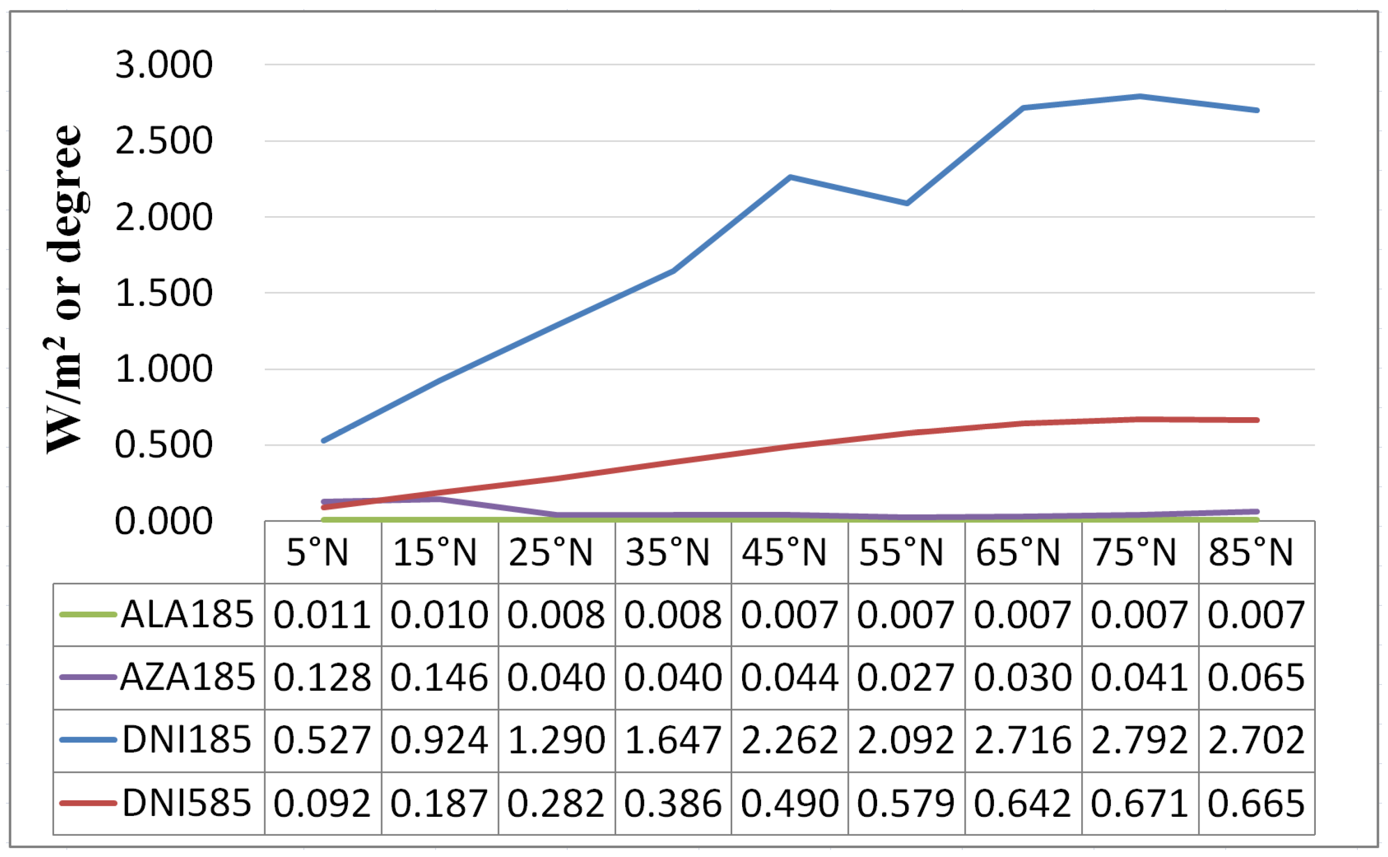
First, DNI, solar altitude angle, and azimuth angle on a day are interpolated from the values of yesterday and the day after tomorrow. There are 9 points at 120° E and 5° intervals between 5° N and 85° N. The time is hourly during 4:00–12:00 LST on the day of 2–363 in 2022. The simulation of DNI using the DNI model in Part I [1] with . The maximum interpolation errors are shown in Figure 4.

Figure 4.
The errors in the interpolation of DNI, solar altitude angle (ALA), and azimuth angle (AZA) at longitude 120°E and difference latitudes. The numbers “185” and “585” represent that the statistical thresholds are solar angles of 1~85 degrees and 5~85 degrees. This is to remove the opposite solar azimuth. That often appears when the solar altitude angle is very high.
Figure 4 shows that the interpolation errors are very small. The comparison between DNI185 and DNI585 shows that the error in DNI increases at low solar altitude angles in high-latitude regions. Because the errors in the solar altitude angle (ALA185) and azimuth angle (AZA185) do not increase at this time, the increase in DNI errors should be related to the characteristics of the DNI model. Nevertheless, the errors in DNI (DNI185) can be considered negligible.
Therefore, the number of days can be reduced to 1/3 (two days apart) when using the day interpolation method.
The error of this method for Model-3Km and Model-9Km on Taiwan Island in the afternoon of 20 March 2022 was tested. The interval is half an hour. This date is around the vernal equinox, which is the season when the solar position changes most daily. The afternoon was chosen to include the low solar altitude. The simulation using the DNI model in Part I with , DEM90 data, HPFTOA, and 2TPA [1]. The interpolation used the values of 19–22 March 2022.
Figure 5 shows the maximum absolute error in interpolation. The errors for Model-9Km are small, and the errors for Model-3Km are slightly larger, but still acceptable.
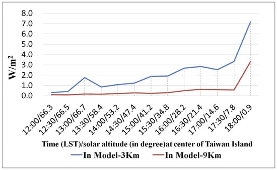
Figure 5.
The maximum absolute error in interpolation on Taiwan Island in the Model-3Km and Model-9Km. The times are half an hour interval during 12:00–18:00 LST in the afternoon on 20 March 2022. The interpolation used data of 19–22 March 2022.
Based on the above analysis, for a year of climate simulation, only 122 days of need to be calculated.
For the study on the Qinghai–Tibet Plateau region of 65–145° E and 0–60° N (80° × 60°) one year, the wall clock time required by using 300 cores of type Gold 6526Y is (44.8 + 50.9)/2 × 122/60/24 × 0.67 = 2.7 days (the ocean area accounts for a third, and it does not need to be calculated). Among them, 44.8 and 50.9 are the wall clocks required to calculate half an hour apart during the whole day of the winter solstice and the summer solstice, respectively (Table 3 in Part I [1]). The size of the data sets for one year with a horizontal resolution of 0.03° × 0.03° will be about 25 GB (processing 32 times per day using an unsigned integer format with 70% compression). This is much smaller than atmospheric model products with the same region and horizontal resolution. If the atmospheric model uses the day of year to calculate the solar position (such as WRF [17,18]), these datasets can be used for a long time. It will be very suitable for open access and has an application field not limited to weather and climate simulations.
The above evaluation shows that, based on HPFTOA and DEM90, the computation cost of the high-precision SPS-CSDSR is feasible for regional weather and climate simulation, even building a data set for the whole year.
Figure 5 shows that for atmospheric models with a horizontal resolution of 3 km, calculating two days apart at mid-latitudes is applicable. For higher resolution and high-latitude regions, further tests are needed based on specific applications. If necessary, calculating one day apart can be used to ensure accuracy.
5. Discussion on Correct Coupling STRE
In mountain areas, the STRE is distributed on the inclined surfaces of a larger area at different heights. This is true of direct solar radiation, scattered radiation, reflected radiation, and long-wave radiation at the surface.
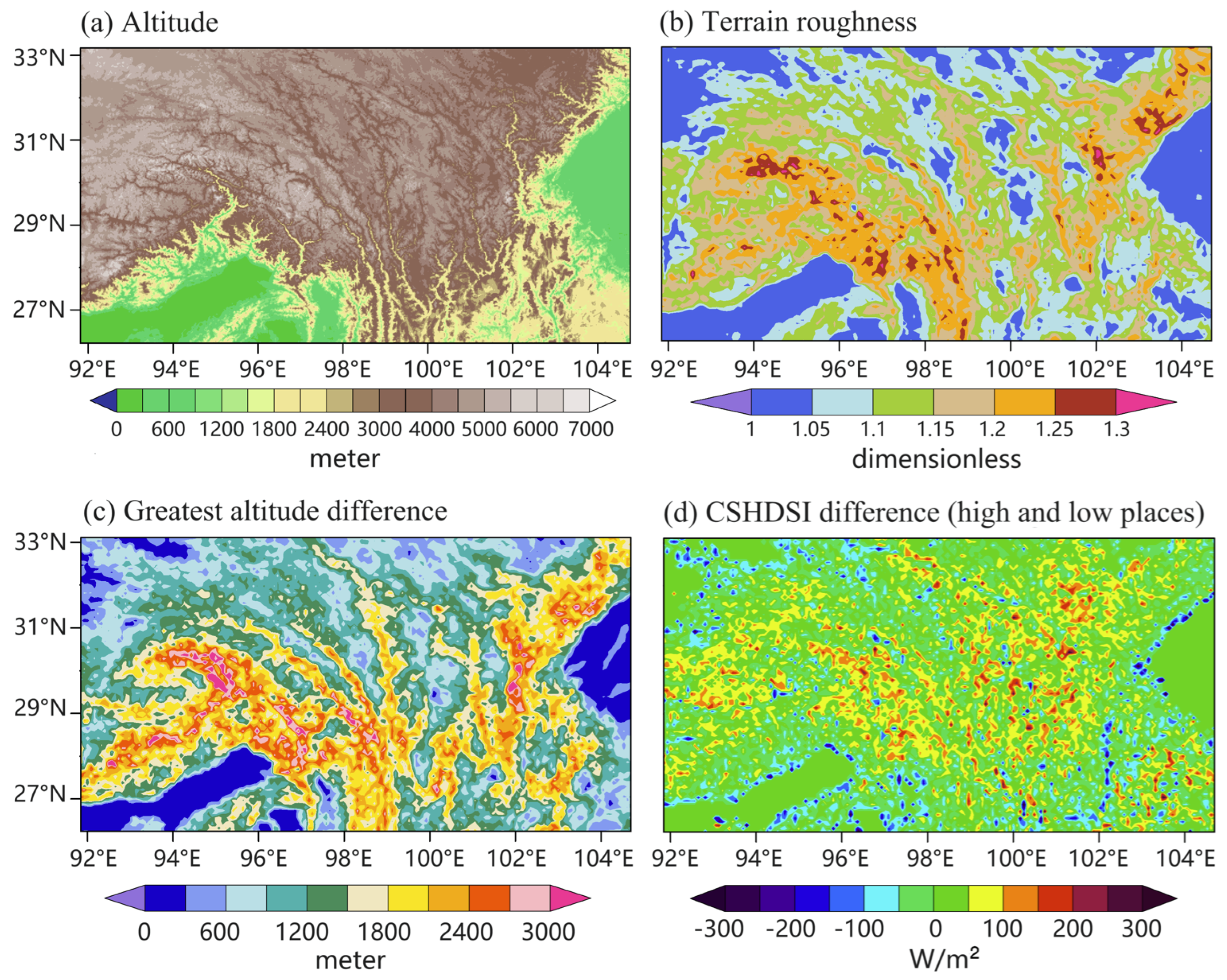
For example, in the south-east part of the Qinghai–Tibet Plateau, with a horizontal resolution of 9 km, the terrain roughness (ratio of surface area to horizontal projected area) of many grid points is above 1.2 (Figure 6b); the land relief within a model grid cell can reach 3000-m (Figure 6b); and sub-grid cells at high places receive more direct solar radiation than the low ones (Figure 6d) because the cast shadows are often at low positions. However, existing land surface physical models are designed for flat land, using real physical parameters such as aerodynamic roughness and emissivity of the surface, heat capacity of the soil, etc.
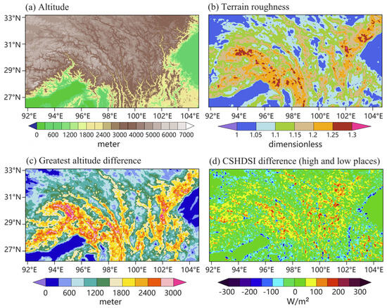
Figure 6.
(a) The altitude of the southeast part of the Qinghai–Tibet Plateau. With a horizontal resolution of 9 km (97 × 97 DEM90 grid cells): (b) the terrain roughness (ratio of surface area to horizontal projected area); (c) the greatest altitude difference of the sub-grid cells within a model grid cell; (d) the difference between above and below the average altitude at 10:00 LST on the Summer Solstice. When the sub-grid cells’ greatest altitude difference is less than 600 m, the difference is set to zero. It was measured on the full horizontal projected area of a mode grid cell, and was made by using HPFTOA, DNI model in Part I with .
Existing methods couple parameterized STRE to the land surface (average height of sub-grid cells) of the atmospheric model. This has certain physical drawbacks. Figure 6d may show a mechanism of mountain fogging: that more solar radiation at the high position of the mountain is conducive to temperature inversions. But when this STRE is introduced to the low position, the exact opposite effect will occur. The horizontal land will also be overheated because its area is smaller than all sub-grid cells. This may trigger convective processes [3].
Some past studies [9,13,14] ignored the increasing surface area of complex terrain, coupling irradiance rather than horizontal irradiance. This led to an underestimation of solar radiation. This may be one reason why these studies concluded that the STRE reduced surface solar radiation in complex terrain.
Therefore, it is necessary to make significant improvements to the atmospheric model coupling STRE. This includes introducing the STRE parameterization to different altitudes and improving coupling between the land surface and atmosphere. This is important for improving the accuracy of simulating high-influence factors on radiation, such as snow cover and terrain clouds (or fogs).
Giorgi et al.‘s [19] mosaic sub-grid method should be used for reference. The method initializes the sub-grids of different heights according to the temperature lapse rate, and then the sensible heat flux of the sub-grid is calculated and synthesized to the height of the model grid cell. This scheme has been used in RegCM3 and RegCM5 [20,21]. In the future, attempts can be made to introduce the sensible heat flux of the sub-grid to several layers. To change this, in Equation (5) in Part I [1] will be limited within some ranges of altitudes. In this case, the sub-grid parameterization schemes of scattered radiation, reflected radiation, and long-wave radiation should also be adapted to it.
For the land surface physical model, it is necessary to consider the difference between the surface area of the plane and the slope. This difference can lead to variations in soil temperature and land-air heat exchange. For example, in Figure 6b, the surface area of many areas increased by more than 20% compared with the plane.
In theory, the parameterization schemes for STRE of short-wave radiation and long-wave radiation must work together. For the high horizontal resolution atmospheric model, due to the presence of the inclined plane, the two-stream long-wave radiation transfer scheme may need to be improved. Three-dimensional outward long-wave radiation transfer may need to be considered. In terms of mechanism and solution, the work of Schäfer et al. [22] and Hogan et al. [23] in respect of representing 3-D cloud radiation effects in two-stream schemes is of great reference significance.
Therefore, the study of correctly expressing the STRE in atmospheric models is still extremely challenging.
6. Conclusions
As for SPS-CSSDSI, after high-resolution DEM data has been widely used, due to the limited computing power of early computers, scholars have proposed three kinds of methods to reduce the amount of computing to promote research in this field. It includes simplified projection shadow processing, assuming the same atmospheric transparency for sub-grid cells, and the cast shadowless coverage method. This study shows that these approximation methods can lead to significant errors.
Despite the huge improvements in current computer performance, the use of approximation algorithms that can lead to large errors has not fundamentally changed before this study. The solutions and verification conclusions proposed in this study solve the above three problems.
In order to solve the problem that SPS-CSSDSI lacks a high-precision and fast terrain occlusion algorithm, the HPFTOA is presented in Part I of this study. It can carry out large-scale computations based on DEM90 with guaranteed accuracy. In this paper, necessary pre-research for the application of the high-precision SPS-CSDSR is carried out. The computational cost can be reduced to 1/3 by using day interpolation. The high-precision SPS-CSDSR is workable for the regional atmospheric model to simulate on a variety of time scales, even building a year-long data set for long-term application. This data set will be very suitable for open access and has an application field not limited to weather and climate simulations. The situation that the past SPS-CSSDSI was severely restricted by terrain occlusion calculations will be fundamentally changed.
This paper analyzes the possible errors caused by assuming that sub-grid cells have the same atmospheric transparency. The result shows that, in undulating terrain, this approximation will lead to significant errors when the sub-grid is in turbid weather or partly above the cloud top, and the latter errors can be more serious. A correction factor is proposed in this paper. It can effectively eliminate errors under a cloudless sky and can reduce some errors when part of the sub-grid is above the cloud or fog top. For the part of the sub-grid above the cloud or fog top, more accurate layering parameterization methods need to be further studied in combination with cloud and fog prediction performance in complex terrain.
For atmospheric models with high horizontal resolution, example test verification shows that the cast shadowless coverage method can lead to significant errors at low solar altitude angles. Although this method has become popular in recent years due to its computational convenience, it should no longer be used based on current computing power.
The improvements in the above three aspects presented in this study will allow SPS-CSDSR to achieve unprecedented high accuracy with few approximation methods.
Reliable downward solar radiation observational data are lacking in mountainous areas [24]. So it is difficult to improve SPS-CSDSR through observation verification. In this case, reducing the use of approximation methods is the main way to ensure the accuracy of SPS-CSDSR.
The application of this high-precision SPS-CSDSR is mainly limited by the resolution of the DEM data. According to the current computer computing power, for large-scale applications of weather model prediction, only DEM data with a resolution no higher than 90 m can be used, and higher-resolution DEM data can be used in smaller ranges and a few times [1]. By not assuming that sub-grid cells have the same atmospheric transparency, the correction factor has a limited effect in weather conditions with low cloud cover (fog). Further improvement in accuracy requires the design of layered parameterization schemes based on the forecasting performance of specific atmospheric models. For the day interpolation method, it is also necessary to determine a reasonable number of interval days based on verification to ensure accuracy.
In mountain areas, the STRE is distributed over inclined surfaces with larger areas and at different heights. Existing methods that couple STRE to the flat land surface of the atmospheric model have certain physical drawbacks. In the future, improvements will need to introduce the STRE parameterization to different altitudes and improve coupling between the land surface and atmosphere. This is important for improving the accuracy of simulating high-influence factors on radiation, such as snow cover and terrain clouds (or fogs).
Therefore, the study of correctly expressing the STRE in atmospheric models is still extremely challenging.
Author Contributions
Conceptualization, C.L. and B.C; methodology, C.L.; resources, B.C. and W.W.; formal analysis, C.L.; writing—original draft preparation, C.L.; writing—review and editing, Y.C., G.F. and X.W.; visualization, C.L.; supervision, B.C. and W.W. All authors have read and agreed to the published version of the manuscript.
Funding
This work was supported by the International Partnership Program of the Chinese Academy of Sciences (Grant N0.134111KYSB20180021), China Meteorological Administration Innovation Development Project (CXFZ2023P023) and the Shandong Provincial Natural Science Foundation (ZR2022MD040).
Institutional Review Board Statement
Not applicable.
Informed Consent Statement
Not applicable.
Data Availability Statement
The raw data supporting the conclusions of this article will be made available by the authors on request. The data are not publicly available due to file sizes. The main computational code is publicly released (https://doi.org/10.5281/zenodo.11402757).
Conflicts of Interest
The authors declare no conflicts of interest.
References
- Li, C.; Wu, W.; Chen, Y.; Feng, G.; Chen, B.; Wen, X. A high-precision sub-grid parameterization scheme for clear-sky direct solar radiation in complex terrain. Part I: A high-precision fast terrain occlusion algorithm. Atmosphere 2024, 15, 857. [Google Scholar] [CrossRef]
- Dubayah, R.; Dozier, J.; Davis, F.W. Topographic distribution of clear-sky radiation over the Konza Prairie, Kansas. Water Resour. Res. 1990, 26, 679–690. [Google Scholar]
- Müller, M.D.; Scherer, D. A grid- and sub-grid-scale radiation parameterization of topographic effects for mesoscale weather forecast models. Mon. Weather. Rev. 2005, 133, 1431–1442. [Google Scholar] [CrossRef]
- Zhang, Y.; Huang, A.; Zhu, X. Parameterization of the thermal impacts of sub-grid orography on numerical modeling of the surface energy budget over East Asia. Theor. Appl. Climatol. 2006, 86, 201–214. [Google Scholar] [CrossRef]
- Essery, R.; Marks, D. Scaling and parametrization of clear-sky solar radiation over complex topography. J. Geophys. Res. Atmos. 2007, 112, D10122. [Google Scholar] [CrossRef]
- Gu, C.; Huang, A.; Wu, Y.; Yang, B.; Mu, X.; Zhang, X.; Cai, S. Effects of sub-grid terrain radiative forcing on the ability of RegCM4.1 in the simulation of summer precipitation over China. J. Geophys. Res. Atmos. 2020, 125, e2019JD032215. [Google Scholar] [CrossRef]
- Helbig, N.; Löwe, H. Shortwave radiation parameterization scheme for sub-grid topography. J. Geophys. Res. Atmos. 2012, 117, D03112. [Google Scholar] [CrossRef]
- He, S.; Smirnova, T.G.; Benjamin, S.G. A scale-aware parameterization for estimating sub-grid variability of downward solar radiation using high-resolution digital elevation model data. J. Geophys. Res. Atmos. 2019, 124, 13680–13692. [Google Scholar] [CrossRef]
- Zhang, X.; Huang, A.; Dai, Y.; Li, W.; Gu, C.; Yuan, H.; Wei, N.; Zhang, Y.; Qiu, B.; Cai, S. Influences of 3D sub-grid terrain radiative effect on the performance of CoLM over Heihe River Basin, Tibetan Plateau. J. Adv. Model. Earth Syst. 2022, 14, e2021MS002654. [Google Scholar] [CrossRef]
- Huang, A.; Gu, C.; Zhang, Y.; Li, W.; Zhang, J.; Wu YZhang, X.; Cai, S. Development of a clear-sky 3D sub-grid terrain solar radiative effect parameterization scheme based on the mountain radiation theory. J. Geophys. Res. Atmos. 2022, 127, e2022JD036449. [Google Scholar] [CrossRef]
- Giorgi, F.; Francisco, R.; Pal, J. Effects of a subgrid-scale topography and land use scheme on the simulation of surface climate and hydrology. Part I: Effects of temperature and water vapor disaggregation. J. Hydrometeorol. 2003, 4, 317–333. [Google Scholar] [CrossRef]
- Hao, D.; Bisht, G.; Gu, Y.; Lee, W.L.; Liou, K.N.; Leung, L.R. A parameterization of sub-grid topographical effects on solar radiation in the E3SM land model (version 1.0): Implementation and evaluation over the Tibetan plateau. Geosci. Model Dev. 2021, 14, 6273–6289. [Google Scholar] [CrossRef]
- Gu, C.; Huang, A.; Zhang, Y.; Yang, B.; Cai, S.; Xu XLuo, J.; Wu, Y. The wet bias of RegCM4 over Tibet Plateau in summer reduced by adopting the 3D sub-grid terrain solar radiative effect parameterization scheme. J. Geophys. Res. Atmos. 2022, 127, e2022JD037434. [Google Scholar] [CrossRef]
- Cai, S.; Huang, A.; Zhu, K.; Guo, W.; Wu, Y.; Gu, C. The forecast skill of the summer precipitation over Tibetan Plateau improved by the adoption of a 3D sub-grid terrain solar radiative effect scheme in a convection-permitting model. J. Geophys. Res. Atmos. 2023, 128, e2022JD038105. [Google Scholar] [CrossRef]
- Jarvis, A.; Reuter, H.I.; Nelson, A.; Guevara, E. The Shuttle Radar Topography Mission (SRTM) 90 m Digital Elevation Database v4.1 [Dataset]. International Centre for Tropical Agriculture (CIAT). 2008. Available online: https://developers.google.com/earth-engine/datasets/catalog/CGIAR_SRTM90_V4 (accessed on 17 June 2023).
- Sharpnack, D.A.; Akin, G. An algorithm for computing slope and aspect from elevations. Photogramm. Eng. 1969, 35, 247–248. [Google Scholar]
- The Official Repository for the Weather Research and Forecasting (WRF) Model. Registry.EM_COMMON.2024, Line 419. 2024. Available online: https://github.com/wrf-model/WRF/blob/master/Registry/Registry.EM_COMMON (accessed on 10 March 2024).
- The Official Repository for the Weather Research and Forecasting (WRF) Model. Module_Radiation_Driver.F. 2024, Lines 3514–3541. 2024. Available online: https://github.com/wrf-model/WRF/blob/master/phys/module_radiation_driver.F (accessed on 10 March 2024).
- Giorgi, F.; Coppola, E.; Solmon, F.; Mariotti, L.; Sylla, M.B.; Bi, X.; Elguindi, N.; Diro, G.T.; Nair, V.; Giuliani, G.; et al. RegCM4: Model description and preliminary tests over multiple CORDEX domains. Clim. Res. 2012, 52, 7–29. [Google Scholar] [CrossRef]
- Pal, J.S.; Giorgi, F.; Bi, X.; Elguindi, N.; Solmon, F.; Gao, X.; Ashfaq, M.; Francisco, R.; Bell, J.; Diffenbaugh, N.; et al. The ICTP RegCM3 and RegCNET: Regional climate modeling for the developing World. Bull. Am. Meteorol. Soc. 2007, 88, 1395–1409. [Google Scholar] [CrossRef]
- Giorgi, F.; Coppola, E.; Giuliani, G.; Ciarlo, J.M.; Pichelli, E.; Nogherotto, R.; Raffaele, F.; Malguzzi, P.; Davolio, S.; Stocchi, P.; et al. The fifth generation regional climate modeling system, RegCM5: Description and illustrative examples at parameterized convection and convection-permitting resolutions. J. Geophys. Res. Atmos. 2023, 128, e2022JD038199. [Google Scholar] [CrossRef]
- Schäfer, S.A.K.; Hogan, J.R.; Klinger, C.; Chiu, J.C.; Mayer, B. Representing 3-D cloud radiation effects in two-stream schemes: 1. Longwave considerations and effective cloud edge length. J. Geophys. Res. Atmos. 2016, 121, 8567–8582. [Google Scholar] [CrossRef]
- Hogan, R.J.; Schäfer, S.A.K.; Klinger, C.; Chiu, J.C.; Mayer, B. Representing 3-D cloud radiation effects in two-stream schemes: 2. Matrix formulation and broadband evaluation. J. Geophys. Res. Atmos. 2016, 121, 8583–8599. [Google Scholar] [CrossRef]
- Chu, Q.; Yan, G.; Wild, M.; Zhou, Y.; Yan, K.; Li, L.; Liu, Y.; Tong, Y.; Mu, X. Ground-Based Radiation Observational Method in Mountainous Areas. In Proceedings of the IGARSS 2019-2019 IEEE International Geoscience and Remote Sensing Symposium, Yokohama, Japan, 28 July 2019–2 August 2019; pp. 8566–8569. [Google Scholar]
Disclaimer/Publisher’s Note: The statements, opinions and data contained in all publications are solely those of the individual author(s) and contributor(s) and not of MDPI and/or the editor(s). MDPI and/or the editor(s) disclaim responsibility for any injury to people or property resulting from any ideas, methods, instructions or products referred to in the content. |
© 2024 by the authors. Licensee MDPI, Basel, Switzerland. This article is an open access article distributed under the terms and conditions of the Creative Commons Attribution (CC BY) license (https://creativecommons.org/licenses/by/4.0/).