Abstract
Accurately generating high-resolution surface grid datasets often involves merging multiple weather observation networks and addressing the challenge of network heterogeneity. This study aims to tackle the problem of accurately interpolating temperature data in regions with a complex topography. To achieve this, we introduce a deterministic interpolation method that incorporates elevation to enhance the accuracy of temperature datasets. This method is particularly valuable for areas with intricate terrains. Our robust methodology integrates a network harmonization method with radial basis function (RBF) interpolation for complex topographical regions. The method was tested on 10 min average temperature data from Jeju Island, South Korea, over 2 years that had a spatial resolution of 100 m. The results show a significant reduction of 5.5% in error rates, from an average of 0.73 °C to 0.69 °C, by incorporating all adjusted data. Integrating a parameterized nonlinear temperature profile further enhances accuracy, yielding an average reduction of 4.4% in error compared to the linear model. The spatial interpolation method, based on regression-based radial basis functions, demonstrates a 6.7% improvement over regression-based kriging for the same temperature profile. This research offers a valuable approach for precise temperature interpolation, especially in regions with a complex topography.
1. Introduction
Near surface temperature is a key variable that is widely used in research on climate change, meteorology, and environmental health. It serves as a crucial indicator of surface energy balance, driving processes like evaporation, sublimation, and snow melting [1,2,3]. Accurate estimation of local air temperature is pivotal for modeling surface processes in physical and environmental sciences.
Gridded temperature datasets are indispensable in various fields, including climate change studies [4,5], crop suitability assessment [6], runoff prediction [7], flood estimation [8], and weather forecasting [9]. However, meteorological stations collecting temperature observations are typically sparse and irregularly distributed, which often hinders accurate estimation of high-resolution grided temperature fields. To overcome this limitation, various interpolation techniques have been proposed, including optimal interpolation [10,11,12,13], the parameter-elevation regressions on independent slopes model (PRISM) [14,15,16,17], and the kriging with external drift (KED) method [18,19,20]. Recently, machine learning-based interpolation methods incorporating auxiliary data, like digital elevation model (DEM) and satellite land surface temperature (LST), have been extensively studied [21,22,23,24,25,26,27]. Furthermore, machine learning methods utilizing satellite data [26] and numerical weather prediction ensembles with field observations have been actively studied [28] for real-time or near-real-time high-resolution temperature interpolation. Our study aims to address the limitations of traditional interpolation methods by introducing a novel deterministic interpolation approach that incorporates elevation data to enhance the accuracy of temperature datasets. Unlike traditional methods, our approach integrates a network harmonization method with RBF interpolation for complex topography. This new method specifically addresses the issue of heterogeneity in weather observation networks, which is a common challenge in traditional interpolation techniques.
Land surface temperature interacts closely with various meteorological parameters, such as wind speed, relative humidity, and atmospheric pressure, playing a pivotal role in shaping weather patterns and atmospheric dynamics. In complex terrains in particular, atmospheric models often exhibit better performance in predicting temperature compared to wind speed due to the challenges posed by the intricate interactions between topography and atmospheric circulation [29,30]. This is attributed to the fact that temperature is influenced by factors such as solar radiation, land–sea distribution, and surface characteristics, which are relatively well represented in models. Recent advancements in observational techniques and modeling approaches have aimed to improve the representation of these interdependencies, leading to enhanced forecast accuracy and a better understanding of atmospheric processes in diverse geographical settings.
An effective approach to estimating temperature at a high resolution is to employ comprehensive data created by integrating observations from multiple networks. However, heterogeneous networks may introduce notable biases, even among equipment that is closely located, due to non-standardized environmental conditions (such as installation altitude and exposure environment) and equipment performance factors (resolution and available measurement range). Nevertheless, even in the most challenging scenarios, the overall error estimation should not be larger than that based on a single network. To address this challenge, it is essential to eliminate heterogeneity among networks. This can be achieved by defining and analyzing the differences among the observed values of networks. A previous study addressed this issue by defining differences among observed values between networks that shared a region and then leveraging these differences to mitigate heterogeneity in observation network data for European gamma dose rate measurements [31]. The results demonstrated that this proposed method reliably identified and quantified biases. After adjusting the estimated biases, the resulting interpolation map was shown to be more reliable than one generated based on the original data.
In mountainous regions, the distribution of surface air temperature presents distinctive horizontal gradients and nonlinear changes with terrain heights, posing a significant challenge for generating temperature datasets across general grids. Moreover, the sparse distribution of stations exacerbates the difficulty in capturing the complex temperature variations in mountainous terrain regions. To address this challenge, incorporating data from additional networks or auxiliary observation networks has been proven to improve the quality of temperature grid datasets in mountainous areas. Several advancements have been made to construct regional high-resolution temperature datasets, including some approaches based solely on station data. For instance, FORBIO (FORest-based BIOeconomy) grid climate data for the daily minimum and maximum temperatures in Belgium were obtained using the KED method [32]. Additionally, the study identified topography as a more critical auxiliary variable compared to land cover type. Brunetti et al. compared three interpolation methods [16]: multilinear regression with local improvement [33], regression kriging (RK), and PRISM-based locally weighted linear regression (LWLR). The findings revealed that LWLR, which considered the relationship between temperature and elevation, provided slightly superior results in estimating monthly temperatures in complex areas. These studies mainly focus on generating data with temporal resolutions such as monthly [16,25,33] or daily [21,30,32,34], with spatial resolutions ranging from 1 km.
A pioneering approach for spatially interpolating the daily air surface temperature in alpine station measurements was introduced in [34]. This method is a deterministic, two-dimensional interpolation method with distance weighting that is modified by using nonlinear parametric profiles and a non-Euclidean distance weighting scheme. These improvements allow for the modeling of the inversion layer in terms of height, contrast, thickness, and adaption to various representation patterns of station measurements under varying meteorological conditions. The flexible approach was rigorously tested in a mountainous region in Switzerland, utilizing daily measurement data from 70 to 110 stations over the period 1961–2010.
Radial basis function (RBF) interpolation is a deterministic interpolation method that is widely used for general and flexible interpolation in multi-dimensional spaces. It is well known for its strong approximation properties and ease of implementation, making it useful not only for approximating statistical and neural networks [35,36] but also for finding approximate solutions to numerical partial differential equations [37,38]. There are several types of RBFs, and selecting an appropriate function and optimal shape parameter based on the density of observation points can ensure the stability and accuracy of the linear equation [39,40,41]. The commonly used Gaussian RBF is sensitive to the shape parameter and has a narrow range of shape parameters with minimal errors, making it difficult to find the optimal shape parameter in each situation [42]. In contrast, the thin-plate spline RBF does not require a shape parameter but may not be as accurate as RBFs that do use shape parameters [39]. Previous meteorological studies have primarily used these Gaussian RBFs or thin-plate splines, resulting in less favorable validation outcomes [43] and a preference for kriging methods over RBFs. In another study [44], four interpolation methods for rain gauge precipitation were compared: inverse distance weight (IDW), RBF, ordinary kriging (OK), and a compressed-sensing method using RBF. The RBF interpolation method showed the smallest error in leave-one-out cross-validation (LOOCV). Instead of using Gaussian or thin-plate RBF, the study used Hardy’s multiquadric RBF and inverse multiquadric RBF, selecting optimal shape parameters to enable precise RBF interpolation. Thus, selection of appropriate RBF and shape parameters has a significant impact on the accuracy of the RBF interpolation method. Before conducting this study, we tested several RBF methods (Gaussian, thin-plate spline, inverse multiquadric, multiquadric, radial powers, etc.) using air temperature data (see Appendix A).
This study aims to develop a fast and accurate method for generating surface air temperature grid data with high spatial (0.1 km) and temporal resolutions (10 min) in a region with a mountainous terrain using multi-heterogeneous observation networks. Drawing inspiration from techniques outlined in [31,34], we merge data from different observation networks and incorporate elevation when modeling temperature profiles. The proposed interpolation method for surface air temperature is specifically tailored for application in mountainous terrains with heterogeneous networks.
Section 2 provides an overview of the study area and the datasets used in this study. Also, the data harmonization and interpolation methods are described in this section. Section 3 presents a comparison of LOOCV errors to assess the impact of data harmonization according to temperature profile types and interpolation techniques. Furthermore, it presents an examination of the monthly cross-validation error, monthly inversion strength, and strong inversion occurrence rate of the air temperature on Jeju Island. Section 4 is dedicated to discussion, while Section 5 summarizes the findings and presents the conclusions.
2. Data and Methods
2.1. Data
2.1.1. Study Area
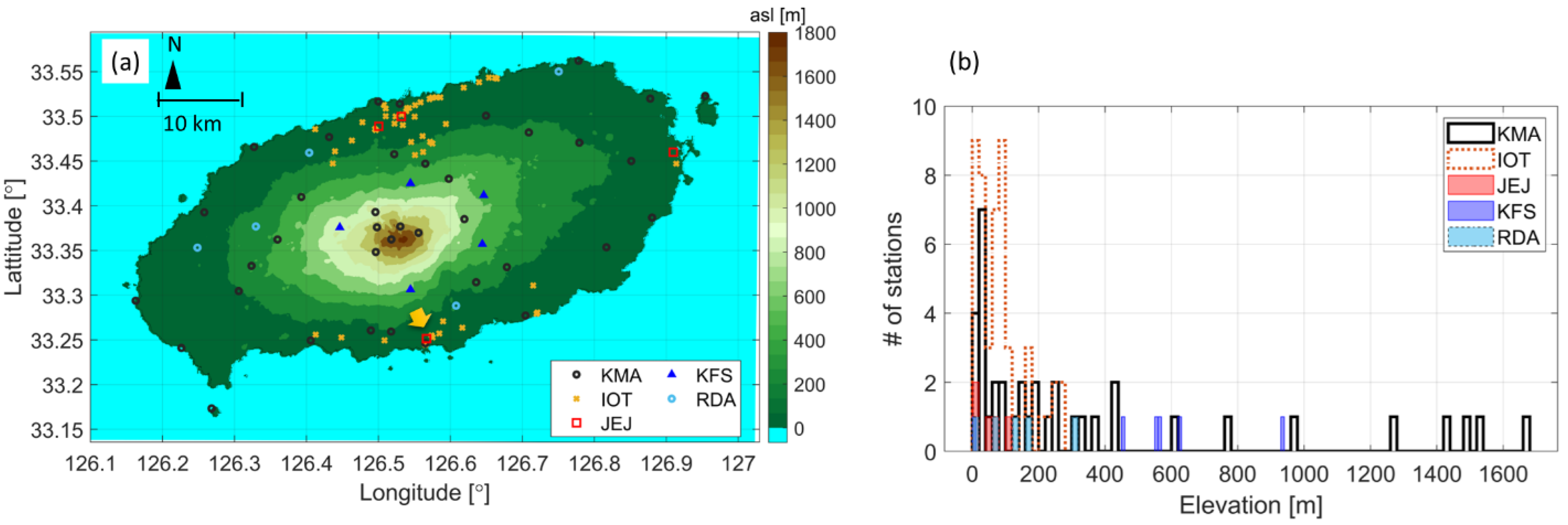
Jeju Island (Figure 1) is a volcanic island that is located on the southern coast of the Korean Peninsula. Covering an area of 1848 km2, it features Hallasan Mountain at its center, a towering volcano with an altitude of 1950 m above sea level (asl). Jeju Island extends 73 km from east to west and 41 km from north to south, corresponding from 33°10′ to 33°34′ N latitude and 126°10′ to 127° E longitude. The island has a humid subtropical climate with cool and dry winters and hot and humid summers [17]. As an island, it is strongly affected by the ocean, resulting in smaller daily temperature variations compared to inland areas, and maintains warm and humid conditions throughout the year. The island has high surface and underground temperatures, making it suitable for horticultural crop cultivation in winter and facility cultivation of subtropical fruit trees. In contrast to inland areas, Jeju Island is characterized by higher temperatures, higher precipitation, and frequent strong winds.

Figure 1.
(a) Study area and locations of stations of the Korea Meteorological Administration (KMA), Korea Forest Service (KFS), Internet of Things (IoT), Rural Development Administration (RDA), and Jeju Province Office (JEJ) used for 10 min temperature interpolation in 2019–2021. The color map represents the digital elevation model (DEM) with 100 m grid spacing in both meridional and zonal directions. The highest grid point and highest station point correspond to 1919 and 1668 m, respectively. (b) The distribution of elevation height for each observation network.
2.1.2. Dataset
A total of five networks were utilized as temperature measurement stations. Figure 1 shows the locations of the stations in the networks along with 100 m resolution DEM data. The utilized networks are maintained by different agencies, such as the Korea Meteorological Administration (KMA), the Korea Forest Service (KFS), the Jeju Province Office (JEJ), and Rural Development Administration (RDA), as well as Internet of Things (IoT) devices. The data output intervals vary depending on the network, i.e., every 1 min for the KMA and KFS, every 5 min for the JEJ and IoT, and every 10 min for the RDA. To synchronize with the RDA’s 10 min interval, the KMA and KFS data were averaged over 10 min periods. For the RDA, since the interval was already 10 min, the data were used as-is at each 10 min mark. For the JEJ and IoT, data received within the past 10 min were averaged, resulting in up to 2 data points being averaged since their intervals were 5 min.
The KMA manages 539 automatic weather stations (AWSs) and 98 Automated Surface Observing Systems (ASOSs) installed throughout South Korea. These stations are distributed spatially in approximately 13 km intervals, with a temporal resolution of 1 min. They continuously collect data on precipitation, air temperature, relative humidity, and air pressure every minute. The temperature and humidity observation equipment is typically installed at a height of about 1.5 m. On Jeju Island, there are a total of 38 KMA datapoints (refer to Figure 1), six of them are located at altitudes of 1000 m or higher.
The IoT devices for weather monitoring are installed in various locations, including schools, government offices, bus stops, town halls, apartments, terminal, and marts. These locations are mainly installed in urban areas, making them susceptible to the influence of the surrounding urban environment, with inconsistent installation heights. The observed measurements include relative humidity, sea level pressure, air temperature, and daily cumulative precipitation. Air-temperature data measured by IoT sensors are acquired at approximately 5 min intervals from a total of 48 sites between July 2019 and June 2021. However, installation height data for each location are not provided. Over the two-year data collection period, the IoT sensors were both removed and newly installed, resulting in fewer than 10 sites performing continuous data collection for the entire duration. Consequently, the number of IoT data collected every 10 min ranges from about 10 to 30 stations during the study period.
The JEJ manages observation data at around 66 locations, but only five stations in the JEJ network monitor temperature observation, recording relative humidity, wind, and daily cumulative precipitation at 5 min intervals as well. The temperature equipment is installed at a height of around 1.5 m.
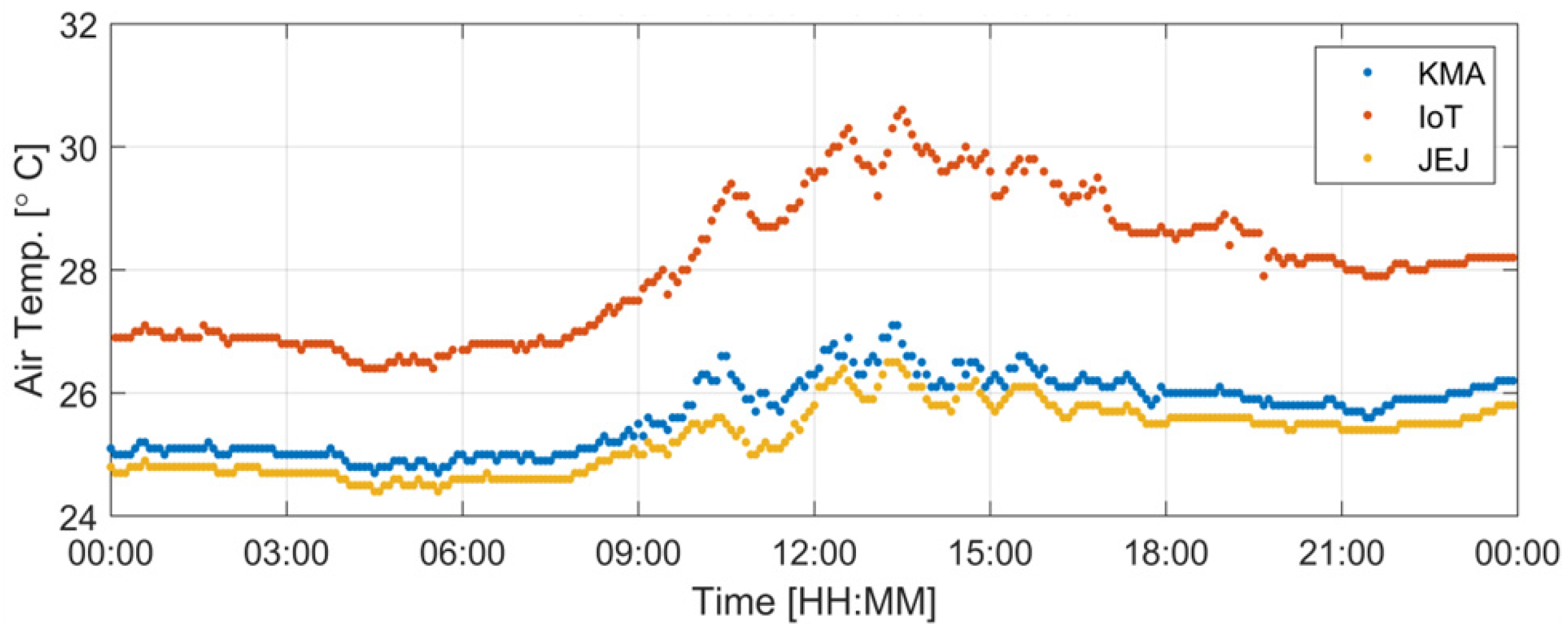
Figure 2 shows the time series of temperature data from closely located IoT, JEJ, and KMA sites (the yellow arrow in Figure 1) on 26 July 2019. The horizontal distances between the KMA and JEJ sites and between the KMA and IoT sites measure 707.5 m and 180.4 m, respectively, which are less than 1 km. The temperature observed at the JEJ site exhibited similarities with that at the KMA site, but the temperature observed at the IoT site, which was only 180 m away from the KMA site, was more than 2 °C higher than that at the KMA site. Notably, the temperature discrepancy between the IoT and KMA sites increased for higher temperatures.
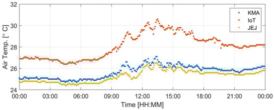
Figure 2.
Temperature time series for 26 July 2019 (LST), for the closest KMA, IoT, and JEJ observation sites, with elevations of 51.86, 83.16, and 50.0 m, respectively. The horizontal distance between the IoT and KMA sites is 180.4 m, while the distance between the JEJ and KMA sites is 707.5 m.
The KFS operates a network of weather stations to monitor precipitation, temperature, relative humidity, and atmospheric pressure at intervals of a few minutes. The stations are typically installed in mountainous areas. There are a total of five observation sites located between 400 and 1000 m asl on Jeju Island (see Figure 1). The temperature observation point for the KFS is at a height of 2 m.
The RDA in South Korea manages observation data of temperature, humidity, wind, and rainfall recorded at 10 min intervals. All five sites in Jeju Island are located at altitudes of 300 m or less, and most of these sites are located far from the AWSs and the city center. The installation height of the temperature observation equipment is 1.5 m, the same as the KMA.
To derive terrain heights for Jeju Island, we used a DEM dataset known as the Global Multiresolution Terrain Elevation Data 2010 with a spatial resolution of 3 arc-seconds. The data were acquired from the website of the United States Geological Survey (https://topotools.cr.usgs.gov/gmted viewer/viewer.htm), last accessed on 5 July 2018.
2.2. Methods
The proposed method comprised three main steps. Firstly, statistical data are generated through temperature data collection for each network. To ensure the quality of heterogeneous network data, statistical data are generated. Following the method outlined in [31], pair data of the values of each network and the interpolated values are compared over a defined period. The collected pair data for each network are then utilized to derive a linear regression equation between the two observation networks.
Secondly, air temperature data for each network is adjusted and removed using these statistical data to eliminate the bias. After establishing a linear regression between the two networks, the “difference” is defined as the distance from this regression equation. Observations with significant differences are then removed, and the heterogeneous network observation data are adjusted using the slope and y-intercept, as detailed in Section 3.2
Lastly, we incorporate the altitude-dependent temperature profile function to perform RBF spatial interpolation on the adjusted data. This interpolation method consists of four steps: (1) Calculating a vertical temperature profile through regression analysis; (2) computing the residuals between the adjusted and merged observed temperature data and the values predicted by the temperature profile; (3) interpolating the residuals; and (4) adding the grid predicted by DEM using the profile to the grid interpolated residual data. It is crucial to note that the DEM must align with the grid information being produced.
The proposed method was validated using surface air-temperature data obtained from five networks in Jeju Island, South Korea, over two years (from July 2019 to June 2021) with spatiotemporal resolutions of 0.1 km and 10 min, respectively. To assess the quantitative accuracy of the method, the LOOCV errors were compared according to the types of elevation profiles and interpolation method.
2.2.1. Interpolation Methods
The main method proposed herein is the interpolation of the residuals after removing the temperature trend with altitude. In this study, RBF and kriging were adopted for interpolation.
Let be the observation at each station . is a continuous function, and we assume that . The RBF interpolation is a deterministic interpolation method that forms a weighted sum of RBFs, as follows:
where is the distance between the interpolated point and the center of each base and is the coefficient or the weight of each RBF . Here, each station point for all networks is used as a center.
Substituting each position in (1), we obtain the following linear equations:
where M is the number of stations. The coefficient matrix is nonsingular and symmetric if is a set of distinct points [45]. By solving the linear equations, we can determine the weights . These weights are used to estimate at an arbitrary position . There are several types of RBFs, such as Gaussian [46], inverse multi-quadratic [46,47], inverse quadratic [48,49], and thin-plate spline [50]. The accuracy of the RBF depends on the type of base functions and shape parameters [39]. In this study, we use the following exponential function [39]:
where is a shape (or scale) parameter. The exponential function was used for interpolating precipitation from rain gauge observations and yielded smaller errors than the commonly used Gaussian RBF [51]. Note that the shape parameter ‘c’ depends on the spatial resolution of stations and the distance units of domain. The shape variable ‘c’ is a variable that determines the radius that affects the surrounding area during interpolation. The larger the value, the larger the radius that it affects. To find the optimal shape parameter and the appropriate RBF, we varied the shape parameters [39,42] and compared the magnitude of LOOCV errors for each method. Among them, the exponential function exhibited a broader optimal shape parameter range than other RBFs that use shape parameters, and it also had smaller errors compared to other RBFs. These analytical results were not included in the main text (See Appendix A). In this study, we used c = 13 km as a shape parameter of the exponential RBF.
Kriging is a geostatistical interpolation method with a linear combination of observations, as follows:
where are the weights that minimize the mean squared error under the constraint that the summation of the weights must be 1; is the prediction value at ; and ) is the observed value at location . The weights ensure that the spatial interpolation is unbiased and has minimal variance. Various kriging methods with different underlying assumptions have been developed. To account for the lack of stationarity, external drifts are often used to model spatially varying trends by decomposing the variable into a trend and a residual , . The trends are linearly modeled with external drifts, and the residuals are assumed to be stationary spatial processes with zero means. In this study, we focused on RK [52,53] and KED [54,55]. Both of these methods use external drifts for modeling spatially varying means. The essential difference between them lies in the computational steps. RK predicts the trend and residuals separately and then adds them to complete the spatial interpolation, as follows:
where is the estimated trend; is the interpolated residual; is the kth external drift at location ; is the corresponding estimated coefficient; is the number of external drifts; is the kriging weight in residual interpolation; and is the residual at location . In this paper, elevation is used as an external drift.
Similar to conventional kriging, the KED predictor is a linear combination of observations, as follows:
where is the weight for the KED under the constraint that for The weights are determined with the extended covariance matrix of residuals and the extended vector of covariances at , including external drifts. Both methods yield the same prediction and prediction variance for the linear trend. Since RK separates trend estimation from residual interpolation, it allows for modeling the trend more flexibly compared to the linear model that is used in KED.
2.2.2. Harmonization Using a Reference Network
KMA AWS data were used as the reference network data for removing and adjusting heterogeneous data (hereafter referred to as harmonization) from multiple observation networks. The reference network is considered to provide the most stable and reliable data among all networks. The first step in removing and adjusting heterogeneities is to predict the values at other network points by interpolating the reference network, the KMA. The selected interpolation method is RBF, and the residual interpolation method is implemented using a fixed temperature lapse rate, 6.5 °C km−1 (see Section 2.2.3). To validate the reference data, it is essential to ensure the reliability of the interpolation process. The verification of this interpolation method utilizes LOOCV, and the results are consistent with those obtained by interpolating the KMA data to validate the KMA network.
A linear relationship is established by comparing the predicted values with the actual observed values. Reliable statistical data are obtained by collecting the observed temperature data over a period of time. The values that exceeded a certain distance are removed using the standard deviation of the distances obtained from the linear relationship. Bias is removed by adjusting the data using the slope and y-intercept of the regression line. The method used is described in detail in the following paragraph.
Let be the observed value at location in network (i = 1, …, M) and be the prediction (or interpolated value) using the observed data from the reference network. For each network , a linear regression is used to model the relationship between and : , where and are the regression coefficients for network and is the total number of stations in network . To determine the deviation from the reference network, we measure the distance between the regression line and the observed value ). When this distance exceeds a predetermined threshold, we regard the corresponding observation as a heterogenous value and eliminate it. In this study, the predetermined threshold was set to , where is the standard deviation of . After the heterogenous data are removed, the observed values in the network are adjusted to remove any bias with the reference network:
This adjustment is performed after removing the heterogenous data to eliminate any bias caused by variations in observation environments among the different observation networks. Specifically, there is a high possibility that the IoT observation data do not comply with the standard installation environment, unlike the KMA observations that are measured in a standard observation environment. Hence, there might still be bias in the observed value.
2.2.3. Computation of Vertical Temperature Profiles
Jeju Island exhibits noticeable temperature variations with altitude because of the presence of Hallasan Mountain, which stands at an altitude of 1900 m and is located at the center of the island. To interpolate the temperature values that are widely dispersed spatially, it is essential to use an altitude-dependent temperature profile. In this study, three types of profiles were compared ((1) a linear equation using a tropospheric mean temperature lapse rate of 6.5 °C km−1, (2) a linear regression using real-time temperature data and altitude, and (3) a real-time nonlinear equation that can simulate an inversion layer) for regression-based interpolations.
Two types of linear temperature profiles were used. The first profile is , with a fixed lapse rate of 6.5 °C km−1, where z (km) is the altitude and is the average temperature at the sea level . The second profile is the real-time linear regression equation, , where and are obtained as different values each time through linear regression.
A nonlinear vertical thermal profile model in [34] that represents an inversion layer with two linear and one nonlinear section is presented as follows:
The linear sections consist of one section at an upper level above elevation and another at a lower level below elevation . These sections share a common lapse rate, . A schematic of the nonlinear parametric function is shown in Figure 3. To determine the five parameters and at each time step, we utilized MATLAB’s nonlinear curve fitting function, ‘lsqcurvefit’, which employs the least squares method.
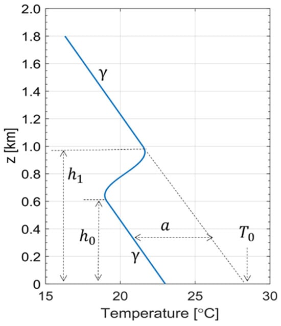
Figure 3.
Schematic of the parametric function of Equation (1) used for a nonlinear vertical profile and its five parameters: and . The two sections are separated by a temperature contrast and are connected in the mid-elevation range by a smooth step function that mimics an inversion layer. Note that this function allows the flexible modeling of inversion-type temperature profiles with adjustable inversion strength (using parameter “a”), height, and thickness (using and ) (see Figure 4 in [34]).
2.2.4. RBF Interpolation Using Real Time Vertical Temperature Profile
The RBF interpolation method is highly effective in estimating function values at arbitrary points. By selecting the observation points as centers, the values at these points can be interpolated with high accuracy. Additionally, choosing a basis function that matches the characteristics of the observed variable and selecting shape parameters based on the density of the observation data and grid resolution can yield more accurate results compared to kriging-based methods [44]. However, when using observation points as centers in the RBF interpolation method, overlapping points should be avoided. If overlaps occur, the overlapping points should either be replaced with an average value or one of the points should be removed.
The RBF interpolation method used in this study involves three steps. First, the vertical-temperature profile is estimated at each time step, where is the altitude and is time. In the next step, each residual at the station point is computed, and these residuals are interpolated in a high-resolution grid . Finally, the temperature field at an actual altitude is obtained by adding the interpolated residual field to the grid field in which the DEM data are substituted for elevation:
The proposed interpolation method considers the surface air-temperature field as a superposition of a simulated background temperature pattern with only elevation information and a residual pattern interpolating the residuals at actual station points. The face temperature field generated in this way is almost identical to the actual value at the network point, and, as the distance from the point increases, it has characteristics that match the value of the background field rather than the observed value. Therefore, in interpolation using residuals, the higher the density of observation points and the more accurate the background fields that are used, the higher the accuracy. In the first step, a separate process is conducted to create the vertical temperature profile, allowing for methodological flexibility through various temperature profile generation tests.
3. Results
In this study, we applied the proposed methodology to the temperature data collected from five observation networks installed on Jeju Island. To establish the criteria for removal and adjustment, we analyzed a two-year dataset spanning from July 2019 to June 2021. The criteria were applied to a one-year dataset covering January to December 2020. Through cross-validation, we assessed the effectiveness of removing and adjusting heterogeneous observations as well as the impact of temperature profiles and interpolation methods on the results.
3.1. Data Harmonization (Removal and Adjustment of Heterogeneous Data)
In establishing the criteria for data harmonization, we gathered interpolated values utilizing KMA AWS and observed values from other observation networks. The interpolation technique employed was RBF, with a fixed lapse rate of γ = 6.5 °C km−1 (as detailed in Section 3.3), to generate the reference dataset.
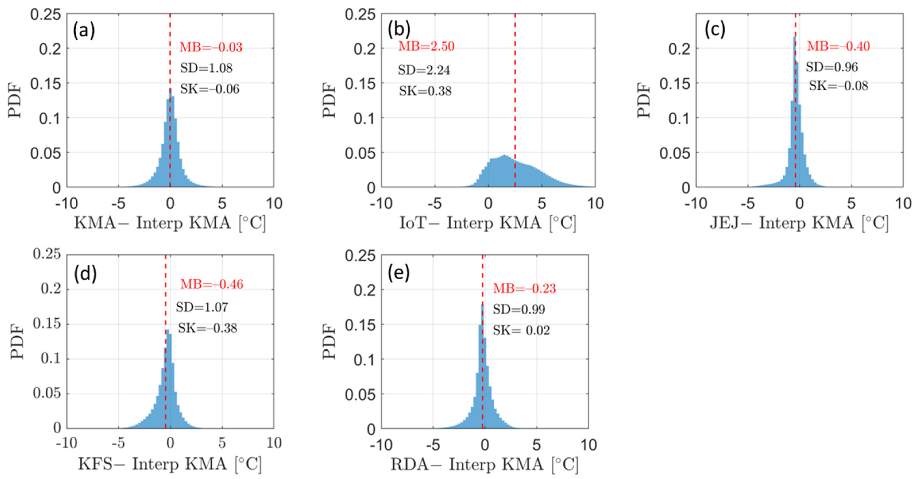
Figure 4 shows the differences between the observed values for each network and the values interpolated using the KMA data. In Figure 4a, the LOOCV values for KMA data are compared with the observation values. The KMA data exhibit the least bias, while the IoT data show a positive distribution with mean bias (MB) of 2.72 °C compared to the KMA data. The data from JEJ and RDA are nearly symmetric, with JEJ showing the smallest standard deviation (SD) value, 0.96 °C. In contrast, the distributions of IoT and KFS data exhibit slight skewness, with Pearson’s skewness coefficients (SK) of 0.38 and −0.38, respectively. Especially, the heterogeneity appears to be pronounced in IoT due to the wide distribution range of data values.
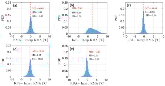
Figure 4.
Distribution of values obtained by subtracting the reference data (i.e., interpolated KMA data) from the data of each network, (a) KMA, (b) IoT, (c) JEJ, (d) KFS, (e) RDA.
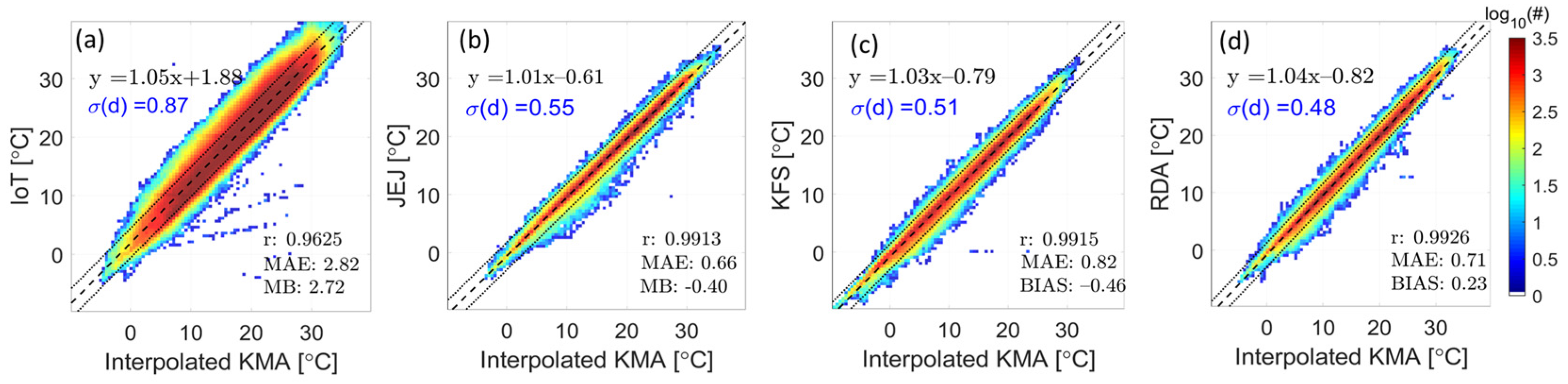
Figure 5 shows the correlation coefficient (, mean absolute error (MAE), and mean bias (MB) for each network, calculated using the reference data, along with a scatterplot. Here, is the standard deviation of the distances between the observed value at a certain network point and the linear regression line of the scatter plot of the values predicted through the reference network for this point (see Section 2.2.2). IoT data have the smallest correlation, with the standard deviation of distance set measuring 0.87 °C, which is about 1.7 times that of the other data. The standard deviations of distance sets for JEJ, KFS, and RDA are 0.55, 0.51, and 0.48 °C, respectively.
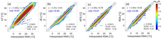
Figure 5.
Scatter plots analysis results for (a) IoT, (b) JEJ, (c) KFS, and (d) RDA data using reference data. The dashed lines are the regression lines from each data series, and the dotted lines are the distance from the regression line for IoT. The remainders are the distances.
The use of the regression function improves the bias but does not enhance the correlation coefficient. The IoT data exhibit a larger standard deviation and lower correlation coefficient than other networks. Therefore, a unique regression equation was derived and adjusted for each IoT device to maximize the adjustment effect. Note that the coefficients of the integrated linear regression equation for the IoT data were 1.05 and 1.88, respectively. Table 1 lists the individual regression equations and bias between each IoT site and the interpolated KMA. The IoT network exhibits distinct characteristics at each station. The specific regressions in Table 1 are used to adjust the data for every station. Notably, all bias values are positive, ranging from 0.27 °C to 5.77 °C across the stations.

Table 1.
Individual coefficient (a, b) and mean bias (MB) and of the Internet of Things (IoT) network data based on the Korea Meteorological Administration (KMA) data for each site.
As shown in the table, it is evident that σ(d) values do not proportionally increase relative to the magnitude of MB; instead, they consistently remain below 1 °C. The presence of these small standard deviations alongside substantial absolute MB values suggests that correcting biases in the data could mitigate errors.
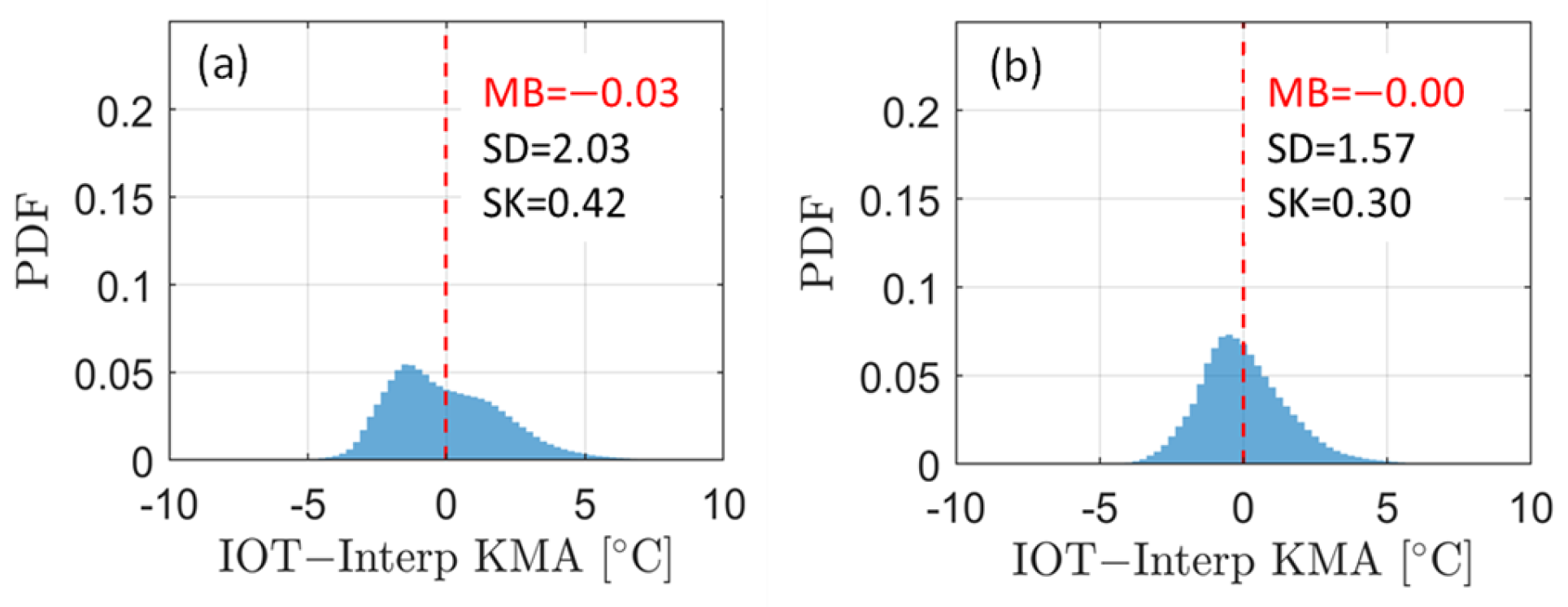
Adjusting for the IoT data using individual linear equations improved the standard deviations compared to adjusting integrated linear equations only. For IoT data, Figure 6 shows the distribution obtained after correction using the coefficient (1.05, 1.88) of integrated linear equation and the distribution after adjustment using the individual linear equations (in Table 1), respectively. According to this distribution, using a single linear equation improved the bias, but significant asymmetries remained. Conversely, after individual adjustments, the data were nearly symmetrical around the mean center.
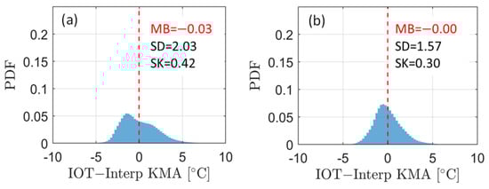
Figure 6.
(a) After adjustment using one integrated linear equation and (b) after adjustment using individual linear lines for each IoT site. The red dashed lines represent the mean bias (MB) values.
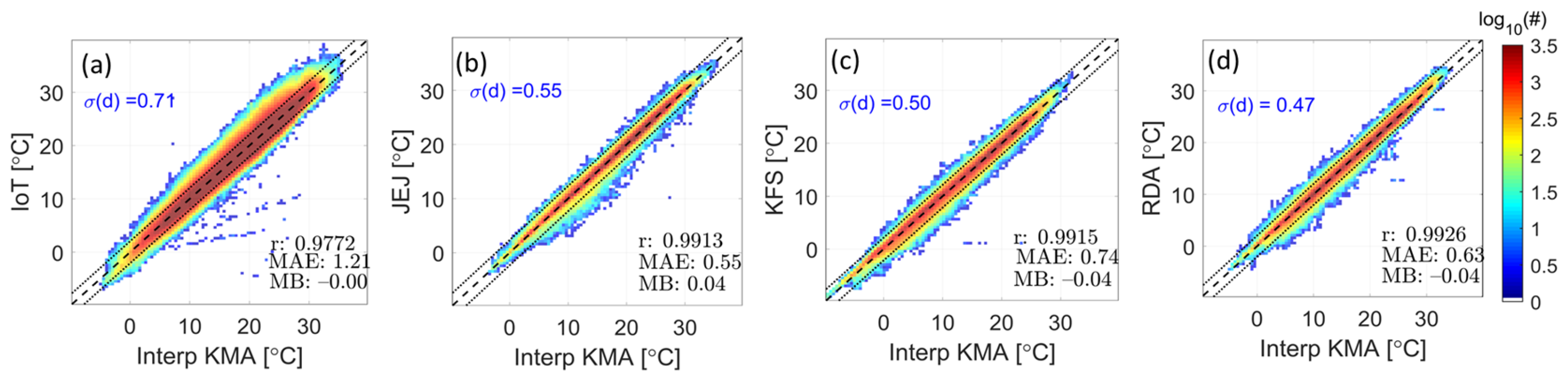
Figure 7 shows scatterplots of the data after only adjustment using the linear regression equation for each network compared with the interpolated KMA data. The plot also depicts the standard deviation σ(d) of the distance to the line y = x after adjustment. In the case of IoT data, individual adjustments increased the correlation coefficient from 0.9626 to 0.9772 and reduced the standard deviation from 0.87 °C to 0.71 °C. However, the MAE was slightly larger (1.21 °C) than that of the other network data. In the cases of the JEJ, KFS, and RDA data, there are negligible changes in the correlation coefficient after correction, and the magnitudes of the MAE and MB decreased slightly after adjustment. Any observations outside of this dotted line are subsequently excluded from further analysis.
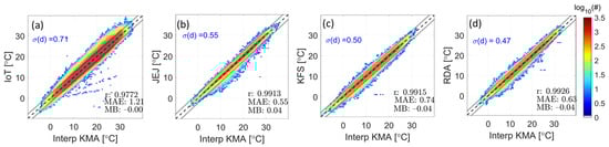
Figure 7.
Scatter plots of (a) IoT, (b) JEJ, (c) KFS, and (d) RDA data after adjustment based on the reference data. Dashed lines: lines for each data, dotted lines: for IoT and distances for the other networks.
Table 2 summarizes the equations used for adjusting each network and the after adjustment. The of IoT was 0.87 °C before adjustment (see Figure 6) and decreased to 0.71 °C after individual adjustment (Table 1). Despite the individual adjustment of the IoT data, values are still relatively higher than those of the other networks. Thus, for data removal, 3σ and 2σ were used as a threshold for IoT and the rest of the networks, respectively. Table 2 also presents the percentage of data removed from the entire data. The removal rates for the IoT, JEJ, KFS, and RDA data are 17.74% (>2σ), 2.82% (>3σ), 5.27% (>3σ), and 4.83% (>3σ), respectively.
Table 2.
Fitting coefficients (a, b) and values for removal and adjustment for each network.
3.2. Verification of Effect of Merging Harmonized Data
To verify the data harmonization effect, RBF interpolation using lapse rate γ = 6.5 °C km−1 was used for comparison.
3.2.1. Examples of Interpolation Results
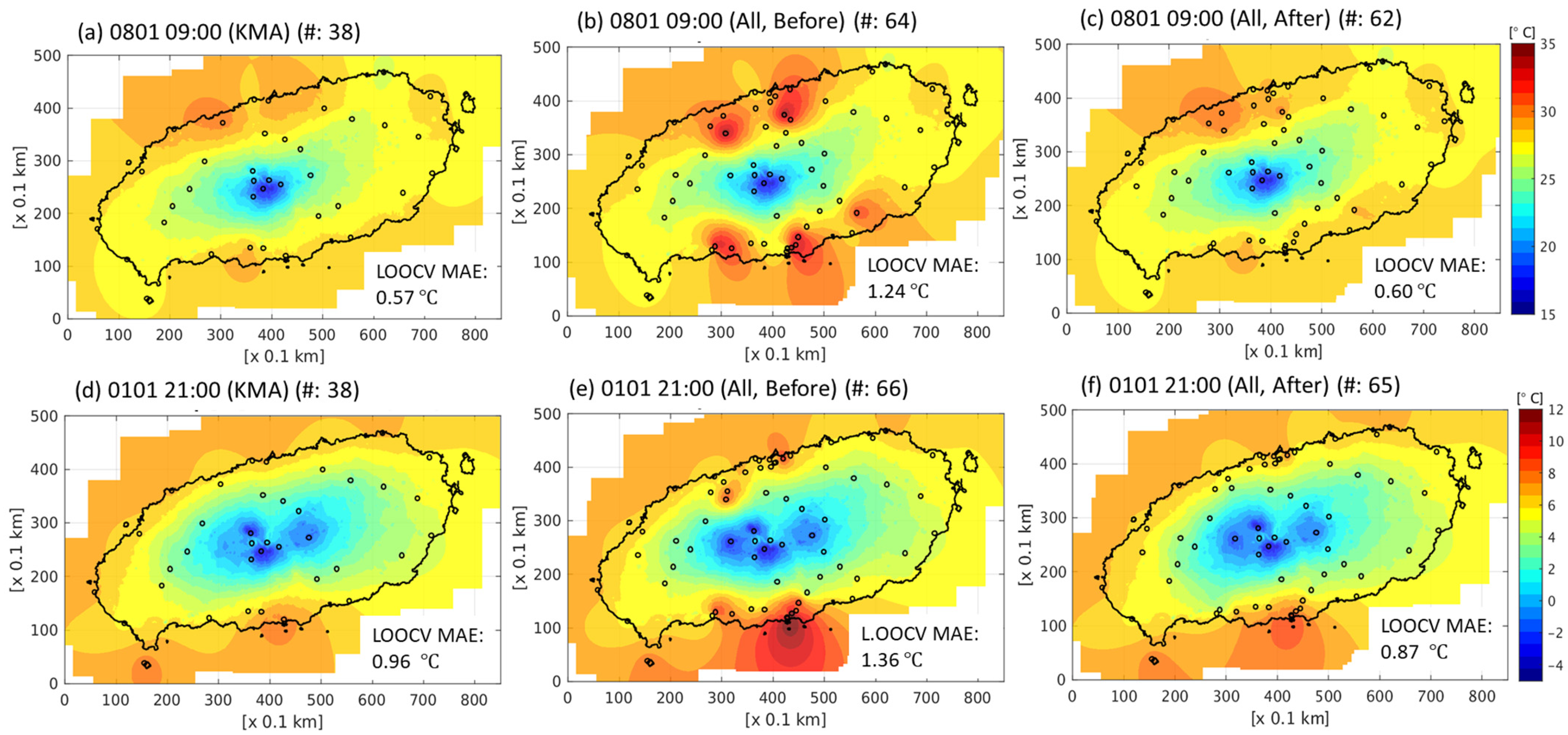
First, we examined cases with and without an inversion layer, randomly selecting two representative cases to assess the impact of merging the harmonized data. Figure 8 shows the interpolated examples for a scenario without an inversion layer. In Figure 8a, a total of 38 KMA data points were used for grid interpolation, resulting in a LOOCV MAE (CVE) value of 0.57 °C. Figure 8b presents the interpolation result based on the combined data from other observation networks with the KMA data, and the CVE increased to 1.24 °C. However, merging the harmonized data with the original KMA data reduced the CVE value to 0.60 °C, as depicted in Figure 8c. Notably, this figure demonstrates the mitigation of the issue, where IoT data were excessively high compared to the surroundings. The interpolation involved 62 points, with two data points removed.
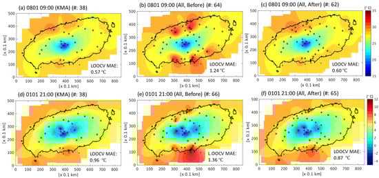
Figure 8.
Grid interpolation images at 09:00 1 August 2020 LST, using (a) KMA data, (b) merged data, and (c) merged data with harmonization, and at 21:00, 1 January 2020 LST, using (d) KMA data, (e) merged data, and (f) merged data with harmonization. The fixed lapse rate of °C km−1 is commonly used as a vertical temperature profile.
Figure 8d–f show interpolation results for the cases involving a temperature inversion layer during the winter of 2020. In Figure 8d, interpolation using only 38 KMAs yields a CVE value of 0.96 °C, which increases to 1.36 °C after merging raw data. After data harmonization, the CVE decreases to 0.87 °C, surpassing the value obtained using only KMA data. In Figure 8, the pixel resolution and grid size are 0.1 km and 850 (longitude) × 500 (latitude), respectively.
3.2.2. Verification Using 2020 Data
To quantitatively assess the effectiveness of removing and merging the adjusted data, 10 min average temperature data were collected at 1 h intervals throughout the year from January to December 2020. We compared the CVE values using the KMA data, the merged dataset of all raw data, and the merged dataset of all harmonized data.
By exclusively utilizing the KMA data from Table 3, the mean CVE over one year is determined to be 0.73 °C. Upon merging the KMA data with those of other networks without harmonization, the mean CVE at KMA stations rises to 1.00 °C, with the average CVE across all merged stations reaching 1.26 °C. However, after merging the data following harmonization processes, the one-year mean CVE for the KMA sites decreases to 0.70 °C and the mean CVE for all data also decreases to 0.69 °C. This confirms that the interpolation error can be mitigated by incorporating the removed and adjusted data during the merging of data from other networks. Additionally, the magnitude of MB value for each network decreases after data harmonization.
Table 3.
Comparison of leave-one-out cross-validation (LOOCV) mean absolute errors (MAEs known as CVEs) before and after data harmonization for a fixed value °C km−1.
3.3. Interpolation Results for Different Temperature Profiles
To compare temperature profiles, RBF interpolation was applied to the removed and adjusted data using the following three temperature profiles: fixed lapse rate, linear regression, and nonlinear regression. Additionally, for a comparative analysis between interpolation methods, CVE values of RBF methods were compared with those of RK and KED.
3.3.1. Examples of Interpolation Results
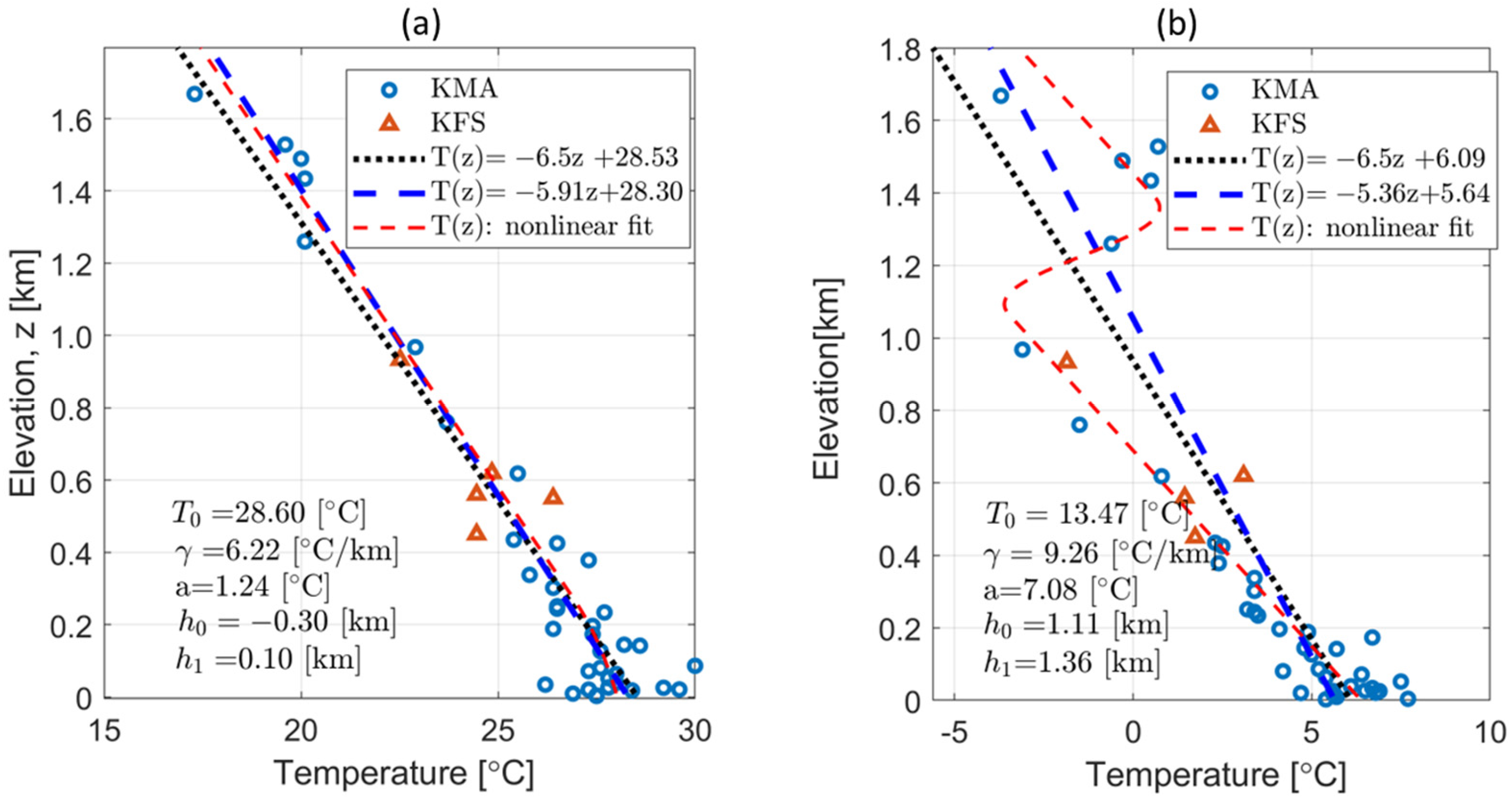
Figure 9 shows the temperature values of the KMA and KFS in relation to altitude along with three types of temperature profiles for two scenarios (with and without inversion). In the absence of an inversion layer (Figure 9a), the slopes of the linear and nonlinear profiles are 5.9 °C km−1 and 6.3 °C km−1, respectively, closely resembling the fixed lapse rate of 6.5 °C km−1. However, with the presence of an inversion layer on 1 January 2020 (Figure 10b), during the winter, the shapes of the three profiles exhibit significant variations. The existence of an inversion layer leads to a lapse rate of only 5.4 °C km−1 in the linearly fitted T(z). The nonlinear equation yields a lapse rate of 9.3 °C km−1 for two separate layers, and the inversion layer has a thickness of approximately 250 m () and a strength of °C.
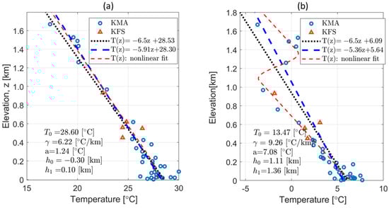
Figure 9.
Examples of vertical-temperature profiles for the following two cases: (a) 09:00 LST, 1 August 2020, without an inversion layer and (b) 21:00 LST 1 January 2020, with an inversion layer. The blue dots and red triangles denote the elevations of the KMA and KFS data, respectively. The black dotted line represents a straight line with a lapse rate of 6.5 °C km−1. The blue dashed line and red dashed curve depict the linear regression line and nonlinear regression curve, respectively.
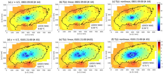
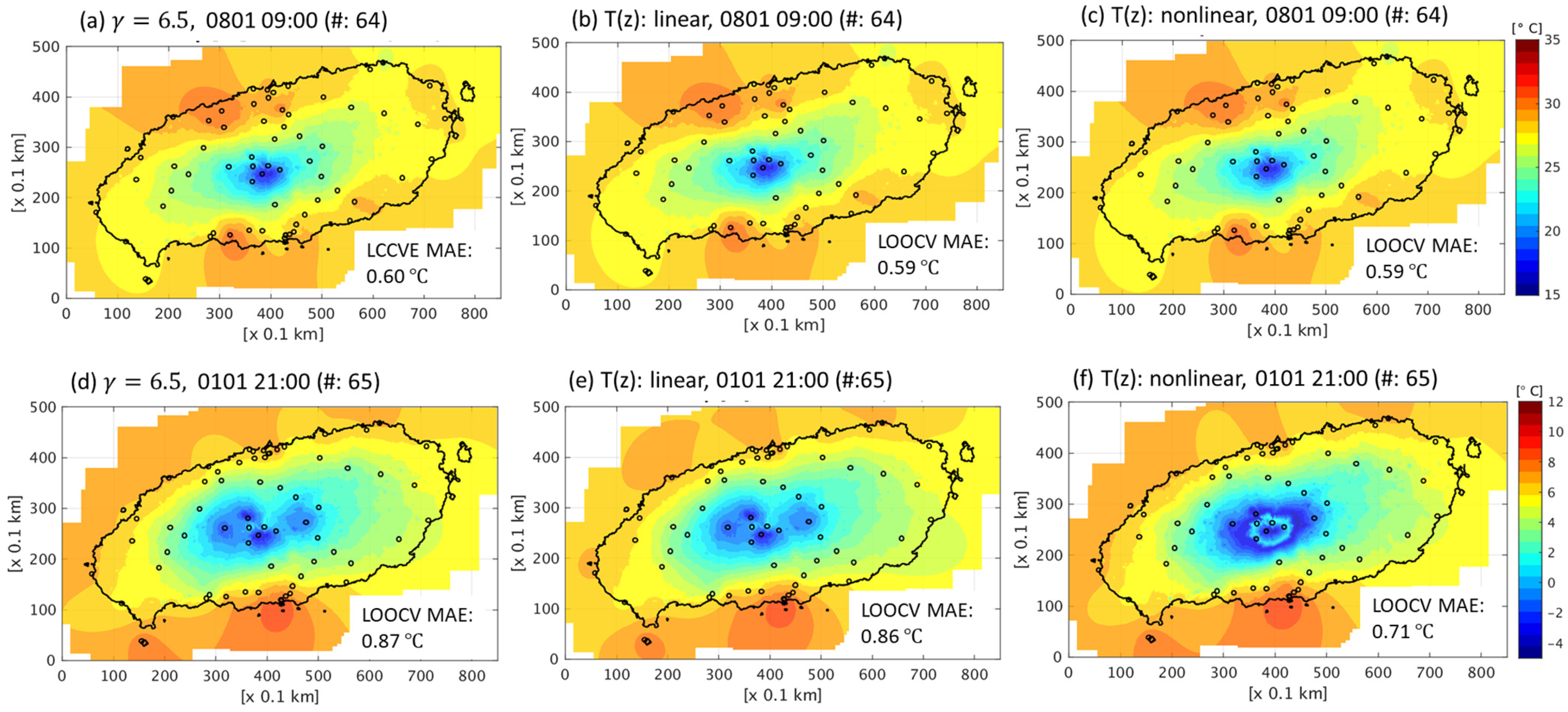
Figure 10.
Grid interpolation images for the harmonized data using different temperature profiles for 09:00 on 1 August 2020 LST (using (a) °C km−1, (b) linear T(z), (c) nonlinear T(z)) and 21:00 LST on 1 January 2020 LST (using (d) °C km−1, (e) linear (f) nonlinear T(z)).
These different temperature profiles are expected to result in varied spatial interpolations. The temperature profiles depicted in Figure 9 were applied to the two aforementioned cases for the data with a harmonization process in Figure 10. In the absence of an inversion layer (Figure 9a), the results of the three temperature profiles, i.e., fixed lapse rate, linear regression, and nonlinear regression, are nearly identical, with CVEs of 0.60, 0.59, and 0.59 °C (Figure 10a–c), respectively. However, in the presence of an inversion layer (Figure 9b), the CVEs of the profiles are 0.87, 0.86, and 0.71 °C (Figure 10d–f), respectively, with the smallest error being obtained using a nonlinear profile. Figure 10f shows a ring-shaped inversion layer at an altitude of approximately 1.2 km asl around the center region of the domain, demonstrating temperature interpolation results that significantly differ from those obtained using a linear temperature profile.
3.3.2. Verification Using 2020 Data
Table 4 presents the CVEs from the 2020 data to evaluate the accuracy of the interpolation methods using different temperature profiles. Additionally, the accuracy of the RBF interpolation is compared with those of RK and KED using the same linear temperature profile.
Table 4.
LOOCV MAE values (CVEs) for different networks and interpolation methods.
When only the KMA data are used, the CVEs of the RBF method with the three temperature profiles (fixed lapse rate, linear regression, and nonlinear regression) are 0.73, 0.72, and 0.66 °C, respectively. After adding all the harmonized data, the errors decrease to 0.69, 0.69, and 0.66 °C, respectively. The interpolation error is minimized when using a nonlinear temperature profile with an inversion layer. The effect of the nonlinear temperature profile is more pronounced when using only the KMA data, probably because the other data, except for the KMA and KFS data, are mostly distributed below an altitude of 400 m and thus are slightly influenced by the altitude.
In comparing interpolation methods, applying a fixed lapse rate of °C km−1 to the KMA data results in CVEs of 0.73 and 0.87 °C for RBF and RK, respectively. Using a linear regression equation, these values become 0.72 and 0.78 °C, respectively. Thus, for the same temperature profile, the error in the RBF is smaller than that of RK. In KED, when only the KMA or all data are used, the CVEs are 0.87 and 0.77 °C, respectively. This result shows that KED provides poorer performance compared to linear RK or RBF.
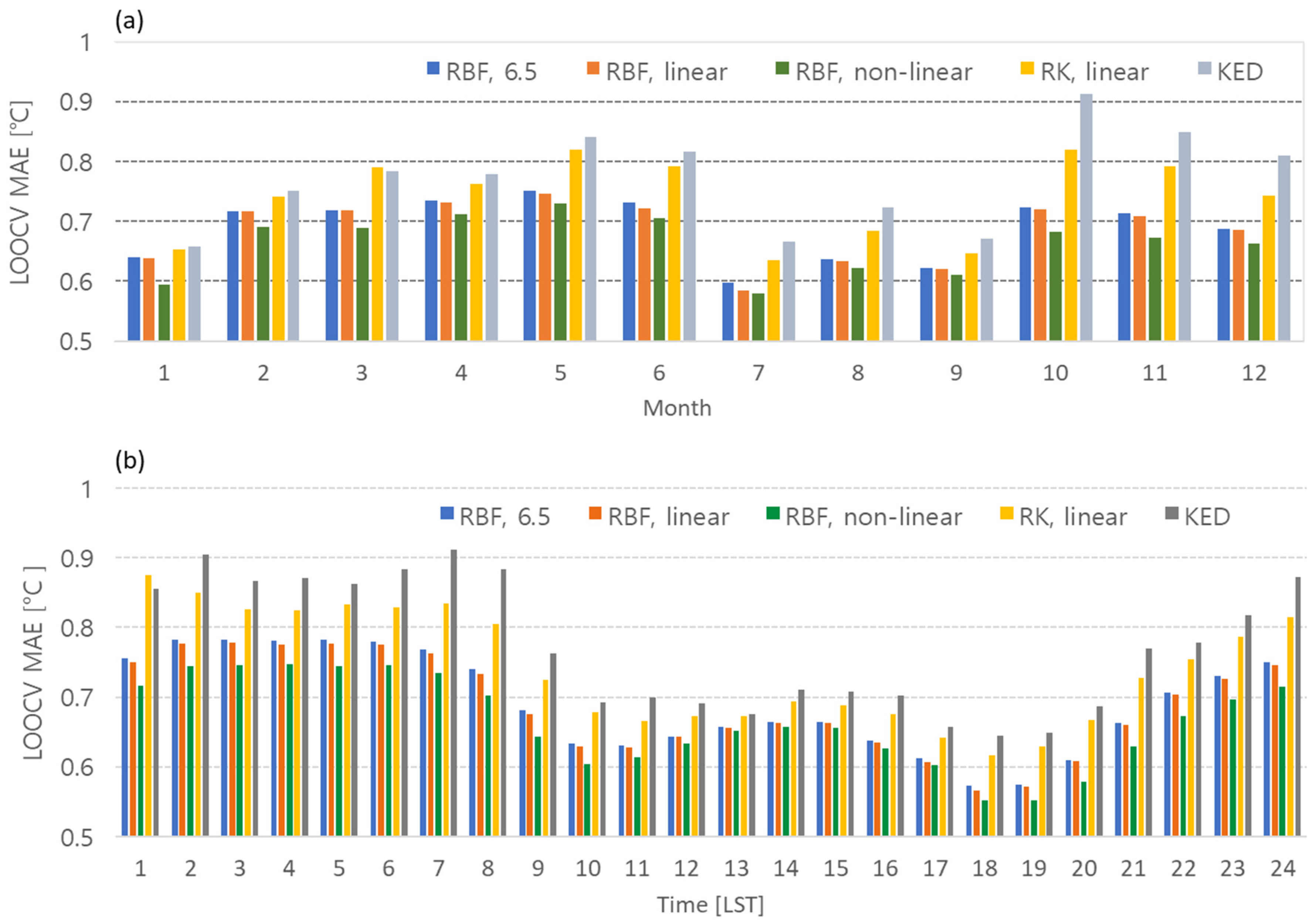
Figure 11 displays the monthly and hourly CVEs for different interpolation methods and temperature profiles. The RBF method using the nonlinear temperature profile consistently exhibits the smallest CVEs for both monthly and hourly error analyses. The RBF method with linear regression has the second-smallest values. Furthermore, the error of RBF is smaller than that of RK for the same temperature profile. Interestingly, unlike the RK method, the RBF method does not exhibit any significant difference in error compared to linear regression when using a fixed average lapse rate of °C km−1.
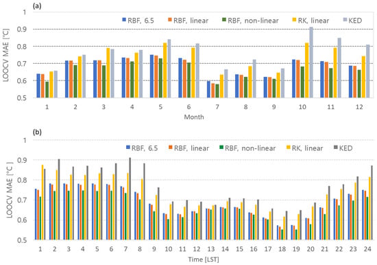
Figure 11.
(a) Monthly and (b) hourly CVEs according to types of temperature profile and interpolation methods.
The monthly CVEs for Jeju Island may be related to the spatial variability of temperature. In other words, the months or hours with relatively large errors across all interpolation methods likely correspond to times when the temperature shows high spatial variability. Overall, the months with the lowest overall CVEs are January, July, August, and September. The average error is the smallest at 0.7 °C or less between 10:00 and 20:00 LST in the hourly results.
The error discrepancy observed between the linear and nonlinear temperature profiles in Figure 11 may be related to the presence or absence of an inversion layer. Specifically, the difference in error between the two temperature profiles is smallest during July, August, and September and between 10:00 and 20:00 LST. This suggests that an inversion layer is less likely to occur in these months and at these times. In January, the difference in error between nonlinear and linear profiles is significant but the overall error is not large. This implies that inversion layers are likely to occur frequently in January but that their spatial variability is not pronounced.
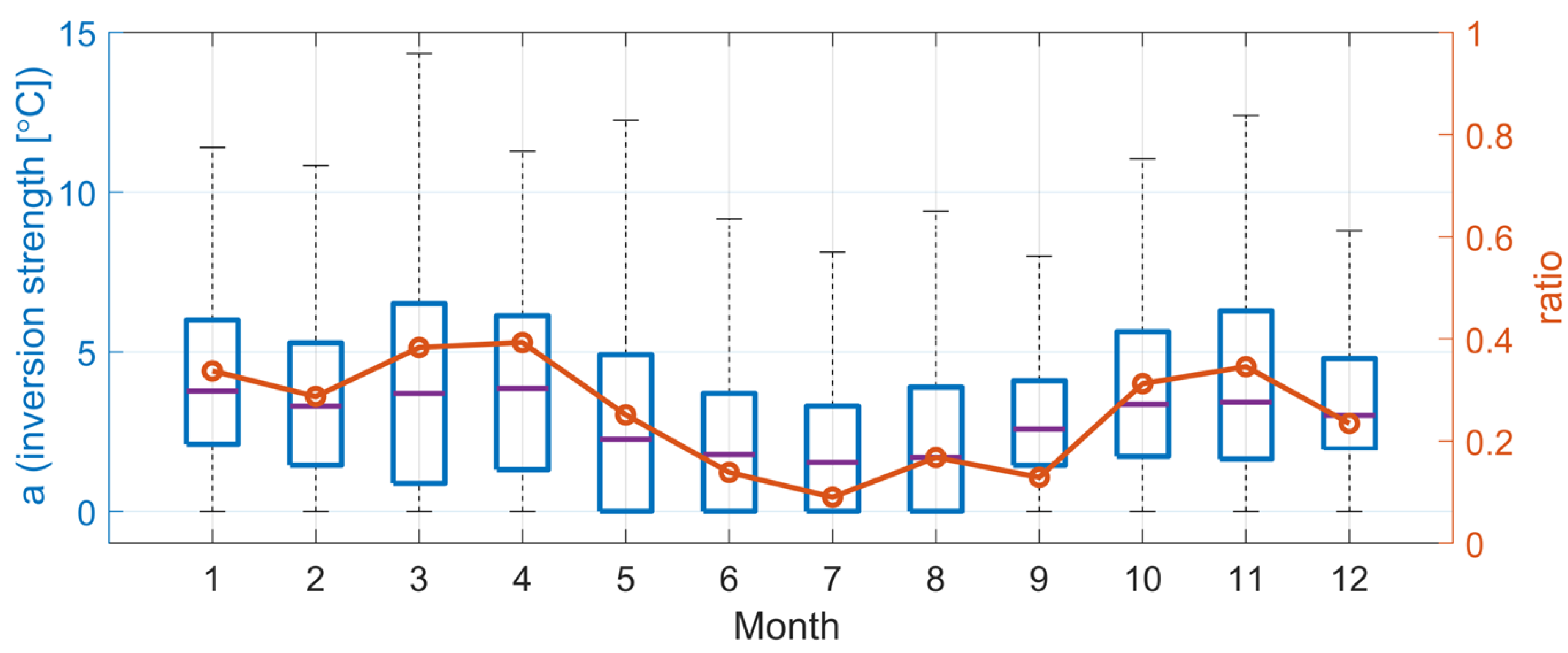
The nonlinear inversion layer modeling discussed in [34] has the advantage of allowing for the identification of both the thickness of the inversion layer and the depth of the temperature change from the resulting profile. Figure 12 shows the distribution of the intensity of the inversion layer occurring between altitudes of 0 and 2 km, as determined by the coefficient obtained from the nonlinear temperature profile and the frequency ratios of cases where °C. The median value of a is the highest at around 4 °C in January and April, while the lowest median is approximately 2 °C in July. The interquartile range (IQR) of the values is the largest in March and May and the smallest in July and September. The possibility of occurrence of a temperature inversion layer with °C is the greatest in March, April, October, and November (30% or more) and the lowest (10%) in July. This finding can explain why the error variation is minimal in July, when both linear and nonlinear temperature profiles are used (Figure 12).
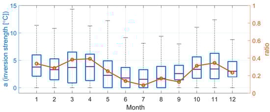
Figure 12.
Monthly distribution of the inversion strength (box plot, left axis) and the incidence rate of cases with a strong inversion of °C (circle, right axis).
4. Discussion
The reduction in error by 5.5% through data harmonization represents a numerical decrease attributed solely to data manipulation. The reduction in LOOCV error was achieved not by altering the interpolation method but by adjusting the heterogeneity across networks through data adjustments. Data adjustment acts similarly to a smoothing effect, thereby reducing errors. Paradoxically, while such methods may decrease validation errors, they can also lead to the production of distorted observational data by removing or reducing outlier values, such as the urban heat island effect in certain regions. Therefore, caution is necessary when adjusting data. In cases where data have low variance and high bias, adjustments using linear regression may be reasonable [56]. However, when dealing with high variance in the data, adjustments may not be necessary to preserve regional characteristics. In such cases, instead of adjusting the data, an alternative approach could be to vary the shape parameter contributing to the influence radius in RBF interpolation based on the LOOCV values at each point [57]. This could reduce errors while preserving peak values in the area. The application of a weighting approach to these shape parameters appears to be reasonable in interpolation and holds potential for future implementation. Identifying the optimal weighting in this method will be crucial.
In this study, the utilization of nonlinear temperature profiles resulted in a 4.4% decrease compared to linear temperature profiles, a figure that may be considered lower than expected. The effectiveness of nonlinear temperature profiles is evident only when temperature inversions occur, with similar errors between the two methods being observed when inversions are absent. Consequently, the overall improvement over one year was not significant. When considering the methodological aspects of kriging and RBF interpolation, the residual-based RBF method shows lower errors compared to residual kriging. Additionally, in the comparison of methods using fixed lapse rates and those employing first-order regression equations to derive temperature lapse rates, there were slightly fewer errors when using first-order regression equations, but the average difference was not substantial.
The methods proposed in this study can be applied beyond Jeju Island to the South Korean Peninsula. Initially, the widespread distribution of AWS data across the peninsula, with the KFS being primarily situated in mountainous regions and the RDA at lower altitudes, provides a foundation. Data fusion is not recommended, particularly for IoT data, due to numerous biased values requiring individual equipment adjustments [58] which may not be cost-effective. Temperature observations are significantly influenced by the installation altitude of equipment and the extent of direct solar exposure. While the KFS and RDA data adhere to standard installation methods like AWS, the IoT data do not. Therefore, by integrating the KFS and RDA with AWS, high-resolution observational data can be obtained. However, due to the larger area and complex terrain compared to Jeju Island, as demonstrated in [30,34], it will be necessary to divide regions by considering local characteristics and apply temperature profiles accordingly.
5. Conclusions
In this study, we introduce a fusion method for temperature data from multiple networks to generate accurate high-resolution gridded data in diverse topographical regions. Our approach harmonizes multiple networks by adjusting biases, removing unreliable data, and using a deterministic real-time temperature interpolation method that incorporates altitude.
Using Radial Basis Function (RBF) with an exponential function, we performed spatial interpolation on 10 min temperature data from five networks in Jeju Island, South Korea. Bias analysis relative to the Korea Meteorological Administration (KMA) data revealed significant discrepancies, particularly for IoT data with an average bias of 2.5 °C. Adjustments were made to eliminate these biases, especially at individual observation stations. To account for altitude variations, vertical temperature profiles were derived from observed values by considering lapse rates and inversion layers.
Quantitative comparisons using leave-one-out cross-validation (LOOCV) errors demonstrated the effectiveness of our method, reducing errors by 5.5% with fixed temperature lapse rates. The method involves generating linear or nonlinear profiles from observed temperatures and station altitudes, interpolating residuals into a grid field. Applying this to an 85 km × 50 km area using DEM grid data minimized errors, with nonlinear profiles reducing average errors by 4.4% compared to linear regression.
Monthly and hourly error analysis revealed distinct differences between linear and nonlinear profiles, except during summer months (July to September) and specific time intervals (10 to 20 LST). We studied the intensity distribution and frequency of monthly strong inversion layers using real-time calculated nonlinear profiles, finding that increased intensity and frequency of inversion layers correlated with higher errors.
In conclusion, our novel temperature interpolation method leverages reference networks to address challenges in combining data from diverse networks. It effectively enhances the accuracy and reliability of temperature data, reducing errors from 0.73 °C to 0.66 °C with nonlinear profiles. Our method’s consideration of nonlinear vertical temperature profiles is particularly advantageous for high-resolution grid interpolation. The successful application to Jeju Island underscores its practical applicability, and its potential extends to other regions with similar topographical challenges, enhancing environmental and meteorological research by improving data integration and analysis accuracy in complex terrains.
Author Contributions
Conceptualization, G.L. and S.R.; methodology, S.R., G.L. and J.J.S.; validation, S.R. and J.J.S.; formal analysis, S.R. and J.J.S.; investigation, G.L. and S.R.; writing—original draft preparation, S.R.; writing—review and editing, G.L., J.J.S. and G.L.; visualization, S.R.; supervision, G.L. All authors have read and agreed to the published version of the manuscript.
Funding
This work was funded by the Korea Meteorological Administration Research and Development Program under Grant KMI2022-00310.
Institutional Review Board Statement
Not applicable.
Informed Consent Statement
Not applicable.
Data Availability Statement
The original contributions presented in the study are included in the article, further inquiries can be directed to the corresponding author.
Acknowledgments
The observation data used in this study was provided by the AI Meteorological Research Division, National Institute of Meteorological Sciences, Korea Meteorological Administration.
Conflicts of Interest
The authors declare no conflicts of interest.
Appendix A
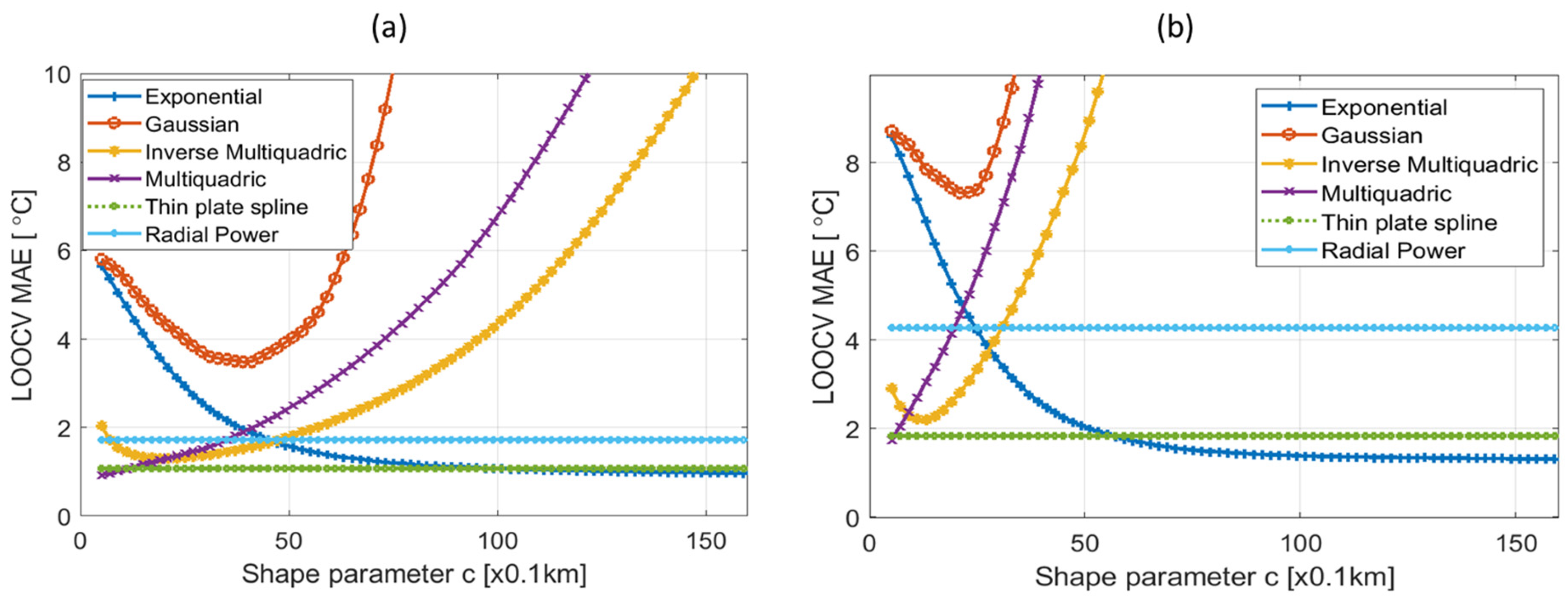
To find the optimal RBF and shape parameter ‘c’ for temperature interpolation, we tested the following RBF functions on the temperature data. The shape parameter was increased from 2 km to 16 km in increments of 0.02, and the MAE values of LOOCV were examined for each shape parameter [39,42].
For the tested RBF functions are:
- Exponential (or Matern):
- Gaussian:
- Multiquadric:
- Inverse multiquadric:
- Radial power:
- Thin-plate spline:
Excluding RBFs not affected by the shape parameter, the value of the shape parameter (c) with the smallest error varied slightly depending on the case. Figure A1 shows the results of calculating the MAE of LOOCV while varying the shape parameter using temperature data fused at two arbitrary times. The Gaussian RBF had the largest error, and it was observed that the error function shape differed depending on the RBF type and the value of ‘c’. In the case of the exponential RBF, it was confirmed that the error stabilized and remained small from approximately c > 10 (km).
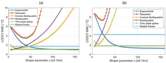
Figure A1.
Examples of LOOCV error tests for merged temperature data at (a) 21:00 1 January and (b) 03:00 13 March 2020 LST.
Figure A1.
Examples of LOOCV error tests for merged temperature data at (a) 21:00 1 January and (b) 03:00 13 March 2020 LST.
References
- Gentine, P.; Chhang, A.; Rigden, A.; Salvucci, G. Evaporation estimates using weather station data and boundary layer theory. Geophys. Res. Lett. 2016, 43, 11661–11670. [Google Scholar] [CrossRef]
- Sexstone, G.A.; Clow, D.W.; Fassnacht, S.R.; Liston, G.E.; Hiemstra, C.A.; Knowles, J.F.; Penn, C.A. Snow Sublimation in Mountain Environments and Its Sensitivity to Forest Disturbance and Climate Warming. Water Resour. Res. 2018, 54, 1191–1211. [Google Scholar] [CrossRef]
- Barnhart, T.B.; Molotch, N.P.; Livneh, B.; Harpold, A.A.; Knowles, J.F.; Schneider, D. Snowmelt rate dictates streamflow. Geophys. Res. Lett. 2016, 43, 8006–8016. [Google Scholar] [CrossRef]
- Ceppi, P.; Scherrer, S.C.; Fischer, A.M.; Appenzeller, C. Revisiting Swiss temperature trends 1959–2008. Int. J. Climatol. 2012, 32, 203–213. [Google Scholar] [CrossRef]
- Van der Schrier, G.; van den Besselaar, E.J.M.; Tank, A.M.G.K.; Verver, G. Monitoring European average temperature based on the E-OBS gridded data set. J. Geophys. Res-Atmos. 2013, 118, 5120–5135. [Google Scholar] [CrossRef]
- Monestiez, P.; Courault, D.; Allard, D.; Ruget, F. Spatial interpolation of air temperature using environmental context: Application to a crop model. Environ. Ecol. Stat. 2001, 8, 297–309. [Google Scholar] [CrossRef]
- Van der Schrier, G.; Efthymiadis, D.; Briffa, K.R.; Jones, P.D. European Alpine moisture variability for 1800–2003. Int. J. Climatol. 2007, 27, 415–427. [Google Scholar] [CrossRef]
- Viviroli, D.; Zappa, M.; Schwanbeck, J.; Gurtz, J.; Weingartner, R. Continuous simulation for flood estimation in ungauged mesoscale catchments of Switzerland—Part I: Modelling framework and calibration results. J. Hydrol. 2009, 377, 191–207. [Google Scholar] [CrossRef]
- Plavcova, E.; Kysely, J. Evaluation of daily temperatures in Central Europe and their links to large-scale circulation in an ensemble of regional climate models. Tellus A Dyn. Meteorol. Oceanogr. 2011, 63, 1052–1054. [Google Scholar]
- Uboldi, F.; Lussana, C.; Salvati, M. Three-dimensional spatial interpolation of surface meteorological observations from high-resolution local networks. Francesco Uboldi, Cristian Lussana and Marta Salvati. Meteorol. Appl. 2008, 15, 537. [Google Scholar] [CrossRef]
- Lussana, C.; Uboldi, F.; Salvati, M.R. A spatial consistency test for surface observations from mesoscale meteorological networks. Q. J. Roy. Meteor. Soc. 2010, 136, 1075–1088. [Google Scholar] [CrossRef]
- Lussana, C.; Tveito, O.E.; Uboldi, F. Three-dimensional spatial interpolation of 2m temperature over Norway. Q. J. Roy. Meteor. Soc. 2018, 144, 344–364. [Google Scholar] [CrossRef]
- Haggmark, L.; Ivarsson, K.I.; Gollvik, S.; Olofsson, R.O. Mesan, an operational mesoscale analysis system. Tellus A Dyn. Meteorol. Oceanogr. 2000, 52, 2–20. [Google Scholar] [CrossRef]
- Daly, C.; Halbleib, M.; Smith, J.I.; Gibson, W.P.; Doggett, M.K.; Taylor, G.H.; Curtis, J.; Pasteris, P.P. Physiographically sensitive mapping of climatological temperature and precipitation across the conterminous United States. Int. J. Climatol. 2008, 28, 2031–2064. [Google Scholar] [CrossRef]
- McGuire, C.R.; Nufio, C.R.; Bowers, M.D.; Guralnick, R.P. Elevation-Dependent Temperature Trends in the Rocky Mountain Front Range: Changes over a 56-and 20-Year Record. PLoS ONE 2012, 7, e44370. [Google Scholar] [CrossRef]
- Brunetti, M.; Maugeri, M.; Nanni, T.; Simolo, C.; Spinoni, J. High-resolution temperature climatology for Italy: Interpolation method intercomparison. Int. J. Climatol. 2014, 34, 1278–1296. [Google Scholar] [CrossRef]
- Um, M.J.; Kim, Y. Spatial variations in temperature in a mountainous region of Jeju Island, South Korea. Int. J. Climatol. 2017, 37, 2413–2423. [Google Scholar] [CrossRef]
- Hudson, G.; Wackernagel, H. Mapping Temperature Using Kriging with External Drift—Theory and an Example from Scotland. Int. J. Climatol. 1994, 14, 77–91. [Google Scholar] [CrossRef]
- Tadic, M.P. Gridded Croatian climatology for 1961–1990. Theor. Appl. Climatol. 2010, 102, 87–103. [Google Scholar] [CrossRef]
- Krahenmann, S.; Bissolli, P.; Rapp, J.; Ahrens, B. Spatial gridding of daily maximum and minimum temperatures in Europe. Meteorol. Atmos. Phys. 2011, 114, 151–161. [Google Scholar] [CrossRef]
- Hengl, T.; Heuvelink, G.B.M.; Tadic, M.P.; Pebesma, E.J. Spatio-temporal prediction of daily temperatures using time-series of MODIS LST images. Theor. Appl. Climatol. 2012, 107, 265–277. [Google Scholar] [CrossRef]
- Stewart, S.B.; Nitschke, C.R. Improving temperature interpolation using MODIS LST and local topography: A comparison of methods in south east Australia. Int. J. Climatol. 2017, 37, 3098–3110. [Google Scholar] [CrossRef]
- Zink, M.; Mai, J.; Cuntz, M.; Samaniego, L. Conditioning a Hydrologic Model Using Patterns of Remotely Sensed Land Surface Temperature. Water Resour. Res. 2018, 54, 2976–2998. [Google Scholar] [CrossRef]
- Collados-Lara, A.J.; Fassnacht, S.R.; Pardo-Iguzquiza, E.; Pulido-Velazquez, D. Assessment of High Resolution Air Temperature Fields at Rocky Mountain National Park by Combining Scarce Point Measurements with Elevation and Remote Sensing Data. Remote Sens. 2021, 13, 113. [Google Scholar] [CrossRef]
- Appelhans, T.; Mwangomo, E.; Hardy, D.R.; Hemp, A.; Nauss, T. Evaluating machine learning approaches for the interpolation of monthly air temperature at Mt. Kilimanjaro, Tanzania. Spat. Stat. 2015, 14, 91–113. [Google Scholar] [CrossRef]
- Ruiz-Alvarez, M.; Alonso-Sarria, F.; Gomariz-Castillo, F. Interpolation of Instantaneous Air Temperature Using Geographical and MODIS Derived Variables with Machine Learning Techniques. ISPRS Int. J. Geo-Inf. 2019, 8, 382. [Google Scholar] [CrossRef]
- Cho, D.; Yoo, C.; Im, J.; Lee, Y.; Lee, J. Improvement of spatial interpolation accuracy of daily maximum air temperature in urban areas using a stacking ensemble technique. GIScience Remote Sens. 2020, 57, 633–649. [Google Scholar] [CrossRef]
- Lussana, C.; Seierstad, I.A.; Nipen, T.N.; Cantarello, L. Spatial interpolation of two-metre temperature over Norway based on the combination of numerical weather prediction ensembles and in situ observations. Q. J. Roy. Meteor. Soc. 2019, 145, 3626–3643. [Google Scholar] [CrossRef]
- Kumar, M.; Kosovic, B.; Nayak, H.; Porter, W.; Randerson, J.; Banerjee, T. Evaluating the performance of WRF in simulating winds and surface meteorology during a Southern California wildfire event. Front. Earth Sci. 2024, 11, 1305124. [Google Scholar] [CrossRef]
- Brinckmann, S.; Krähenmann, S.; Bissolli, P. High-resolution daily gridded data sets of air temperature and wind speed for Europe, Earth Syst. Sci. Data 2016, 8, 491–516. [Google Scholar] [CrossRef]
- Skøien, J.; Baume, O.; Pebesma, E.; Heuvelink, G.M. Identifying and removing heterogeneities between monitoring networks. Environmetrics Off. J. Int. Environmetrics Soc. 2010, 21, 66–84. [Google Scholar] [CrossRef]
- Delvaux, C.; Journee, M.; Bertrand, C. The FORBIO Climate data set for climate analyses. Adv. Sci. Res. 2015, 12, 103–109. [Google Scholar] [CrossRef]
- Hiebl, J.; Auer, I.; Bohm, R.; Schoner, W.; Maugeri, M.; Lentini, G.; Spinoni, J.; Brunetti, M.; Nanni, T.; Tadic, M.P.; et al. A high-resolution 1961-1990 monthly temperature climatology for the greater Alpine region. Meteorol. Z. 2009, 18, 507–530. [Google Scholar] [CrossRef]
- Frei, C. Interpolation of temperature in a mountainous region using nonlinear profiles and non-Euclidean distances. Int. J. Climatol. 2014, 34, 1585–1605. [Google Scholar] [CrossRef]
- Li, J.Y.; Luo, S.W.; Qi, Y.J.; Huang, Y.P. Numerical solution of elliptic partial differential equation using radial basis function neural networks. Neural Netw. 2003, 16, 729–734. [Google Scholar]
- Wei, C.C. RBF Neural Networks Combined with Principal Component Analysis Applied to Quantitative Precipitation Forecast for a Reservoir Watershed during Typhoon Periods. J. Hydrometeorol. 2012, 13, 722–734. [Google Scholar] [CrossRef]
- Safdari-Vaighani, A.; Larsson, E.; Heryudono, A. Radial Basis Function Methods for the Rosenau Equation and Other Higher Order PDEs. J. Sci. Comput. 2018, 75, 1555–1580. [Google Scholar] [CrossRef]
- Liu, Z.Y.; Xu, Q.Y. A Multiscale RBF Collocation Method for the Numerical Solution of Partial Differential Equations. Mathematics 2019, 7, 964. [Google Scholar] [CrossRef]
- Fasshauer, G.E. Meshfree Approximation Methods with MATLAB; World Scientific: Singapore, 2007. [Google Scholar]
- Roque, C.; Ferreira, A.J. Numerical experiments on optimal shape parameters for radial basis functions. Numer. Methods Partial. Differ. Equ. Int. J. 2010, 26, 675–689. [Google Scholar] [CrossRef]
- Mongillo, M. Choosing basis functions and shape parameters for radial basis function methods. SIAM Undergrad. Res. Online 2011, 4, 2–6. [Google Scholar] [CrossRef]
- Fasshauer, G.E.; Zhang, J.G. On choosing “optimal” shape parameters for RBF approximation. Numer. Algorithms 2007, 45, 345–368. [Google Scholar] [CrossRef]
- Katipoğlu, O.M.; Acar, R.; Şenocak, S. Spatio-temporal analysis of meteorological and hydrological droughts in the Euphrates Basin, Turkey. Water Supply 2021, 21, 1657–1673. [Google Scholar] [CrossRef]
- Ryu, S.; Song, J.J.; Kim, Y.; Jung, S.H.; Do, Y.; Lee, G. Spatial Interpolation of Gauge Measured Rainfall Using Compressed Sensing. Asia-Pac. J. Atmos. Sci. 2021, 57, 331–345. [Google Scholar] [CrossRef]
- Powell, M.J.D. Univariate Multiquadric Approximation—Reproduction of Linear Polynomials. Int. S. Num. M. 1990, 94, 227–240. [Google Scholar]
- Buhmann, M. Radial Basis Functions: Theory and Implementations; Cambridge University Press: Cambridge, UK, 2003. [Google Scholar]
- Hardy, R.L. Multiquadric equations of topography and other irregular surfaces. J. Geophys. Res. 1971, 76, 1905–1915. [Google Scholar] [CrossRef]
- Fornberg, B.; Wright, G. Stable computation of multiquadric interpolants for all values of the shape parameter. Comput. Math. Appl. 2004, 48, 853–867. [Google Scholar] [CrossRef]
- Chow, J.Y.J.; Regan, A.C.; Arkhipov, D.I. Faster Converging Global Heuristic for Continuous Network Design Using Radial Basis Functions. Transport. Res. Rec. 2010, 2196, 102–110. [Google Scholar] [CrossRef]
- Morse, B.S.; Yoo, T.S.; Rheingans, P.; Chen, D.T.; Subramanian, K.R. Interpolating implicit surfaces from scattered surface data using compactly supported radial basis functions. In ACM SIGGRAPH 2005 Courses; 2005; pp. 78–87. Available online: https://dl.acm.org/doi/abs/10.1145/1198555.1198645 (accessed on 25 March 2024).
- Lin, G.-F.; Chen, L.-H. A spatial interpolation method based on radial basis function networks incorporating a semivariogram model. J. Hydrol. 2004, 288, 288–298. [Google Scholar] [CrossRef]
- Ahmed, S.; De Marsily, G. Comparison of geostatistical methods for estimating transmissivity using data on transmissivity and specific capacity. Water Resour. Res. 1987, 23, 1717–1737. [Google Scholar] [CrossRef]
- Odeh, I.O.; McBratney, A.; Chittleborough, D. Further results on prediction of soil properties from terrain attributes: Heterotopic cokriging and regression-kriging. Geoderma 1995, 67, 215–226. [Google Scholar] [CrossRef]
- Wackernagel, H. Multivariate Geostatistics: An Introduction with Applications, 2nd ed.; Springer: Berlin, Germany, 1998. [Google Scholar]
- Chiles, J.-P.; Delfiner, P. Geostatistics: Modeling Spatial Uncertainty; John Wiley & Sons: Hoboken, NJ, USA, 2009; Volume 497. [Google Scholar]
- Mehta, P.; Bukov, M.; Wang, C.H.; Day, A.G.; Richardson, C.; Fisher, C.K.; Schwab, D.J. A high-bias, low-variance introduction to machine learning for physicists. Phys. Rep. 2019, 810, 1–124. [Google Scholar] [CrossRef] [PubMed]
- Stolbunov, V.; Nair, P.B. Sparse radial basis function approximation with spatially variable shape parameters. Appl. Math. Comput. 2018, 330, 170–184. [Google Scholar] [CrossRef]
- Sanyal, S.; Zhang, P. Improving quality of data: IoT data aggregation using device to device communications. IEEE Access 2018, 6, 67830–67840. [Google Scholar] [CrossRef]

Disclaimer/Publisher’s Note: The statements, opinions and data contained in all publications are solely those of the individual author(s) and contributor(s) and not of MDPI and/or the editor(s). MDPI and/or the editor(s) disclaim responsibility for any injury to people or property resulting from any ideas, methods, instructions or products referred to in the content. |
© 2024 by the authors. Licensee MDPI, Basel, Switzerland. This article is an open access article distributed under the terms and conditions of the Creative Commons Attribution (CC BY) license (https://creativecommons.org/licenses/by/4.0/).