Moisture Transport during Anomalous Climate Events in the La Plata Basin

Abstract

This paper examines the linear relationship between climate events in the La Plata Basin (LP) from 1980 to 2018 and atmospheric moisture transport from major sources using a Lagrangian approach. The standardized precipitation evapotranspiration index (SPEI-1) was utilized to assess climate events, as monthly water balance variations may be related to changes in atmospheric moisture transport. A total of 49 dry and 46 wet events were identified through sequences of negative and positive SPEI-1 values, respectively. Lagrangian analysis tracked changes in moisture uptake and supply from sources to the LP during these events. Simple linear regression analysis revealed a relationship between moisture transport from the Amazonas (AM), North Atlantic (NA), and Tocantins (TO) basins and the severity and duration of climate events. Increased moisture supply from the São Francisco basin (SF) and Eastern Brazil oceanic (EBO) sources intensified the duration and severity of wet events. Peak wet events were linked to increased moisture supply from the northern South America basins (AM, NA, and TO), while peak droughts were related to decreased moisture uptake from eastern sources (TO, SF, and EBO). Our findings highlight how the water balance in distant regions affects the LP via moisture transport, emphasizing the need for interconnected adaptive strategies.

1. Introduction

The increase in frequency and intensity of extreme climate events is one of the consequences of climate change [1]. In South America (SA), these changes have caused social and environmental issues on the continent, such as modification on water-climate balance [2,3]. Droughts have also contributed to wildfire spreading. For instance, the extreme drought from 2019 to 2021 over the La Plata Basin (LP) [4] facilitated the wildfires in the Pantanal mainly during 2020 [5]. In an opposite way, daily extreme rainfall events are occurring with higher frequency over southern Brazil [6,7], such as those associated with high volumes of precipitation in Rio Grande do Sul state during the austral autumn in 2024, which led to floods and landslides, resulting in severe consequences for the population [8].

Encompassing areas of central and southern Brazil, southeastern Bolivia, Paraguay, Uruguay, and northern Argentina, the LP is the second largest basin in SA. Apart from accommodating a significant portion of the continent’s population and economic activities, its importance as a source of water and hydroelectric power is evident [9]. Studies indicate that changes in rainfall patterns in the basin, coupled with land use changes, have been the primary drivers behind the increased frequency of floods since the 1980s [10,11,12]. Drought is also a recurring phenomenon in the LP, exerting notable impacts across various sectors, including agriculture and hydroelectric power generation [4,10,13].

Extreme climate events significantly impact human society, ecosystems, and economies by deviating from long-term average conditions [14]. Droughts are complex phenomena with varied definitions, complicating their conceptualization and monitoring [15]. Generally, drought is a temporal anomaly relative to long-term climate conditions [16], characterized by below-normal water availability unable to meet existing demand [17]. Drought effects may accumulate slowly, expand over large regions, and impact different stages of the atmospheric water cycle [18]. Due to the different sectors affected by the droughts, these events can be classified into four major categories: meteorological, agricultural, hydrological, and socioeconomic [16]. Meteorological drought is defined by below-average precipitation and may include increased evapotranspiration [19], serving as the primary cause of other drought types [20]. Agricultural drought affects crops via declining soil moisture, hydrological drought reduces water levels in bodies affecting users, and socioeconomic drought limits economic goods due to water shortages. On the opposite side, wet climate events involve abnormal increases in precipitation, including heavy rainfall and prolonged precipitation [14]. These events disrupt local hydrology, agriculture, and infrastructure, potentially causing flooding and landslides.

Climate indices have been serving as valuable tools for analyzing extreme climate conditions. For instance, the World Meteorological Organization recommends the use of the standardized precipitation index (SPI) [21] for operational monitoring of climate extremes [18,22]. The SPI was designed to quantify precipitation (PRE) deficits across multiple timescales, reflecting the impacts of drought on different components of the hydrological cycle. Therefore, the SPI may be a useful tool for accurately identifying the hydrological, agricultural, and environmental impacts of anomalous climate conditions [21,23]. However, other meteorological variables also influence drought conditions, such as evapotranspiration. To address the effect of evapotranspiration, the standardized precipitation evapotranspiration index (SPEI) incorporates potential evapotranspiration (PET) into its formulation [23]. Employing the same conceptual methodology as SPI, SPEI provides a more comprehensive measure of the water balance by accounting for the difference between rainfall and potential evapotranspiration. Numerous studies have applied SPI and SPEI indices to analyze extreme climatic conditions in the LP and southern South America [3,4,13,24,25,26,27].

The role of atmospheric moisture transport from continental sources, including recycling processes and the Amazon, as well as from the South Atlantic Ocean, in influencing precipitation patterns across the LP is known [28,29,30,31,32,33,34,35,36,37]. The techniques currently employed in the analysis of atmospheric moisture transport are presented in [38], and among them, there is the Lagrangian approach [39,40,41,42,43]. This technique enables the tracking of air masses, facilitating more realistic analyses of the source-sink relationship in moisture transport studies. This capability explains the increasing adoption of this method by the scientific community.

Lagrangian analysis of moisture transport in SA has been relatively limited in the literature. Previous studies, such as those by [30,34], have examined climatic regions defined by the Intergovernmental Panel on Climate Change (IPCC). Investigations have targeted specific areas and phenomena, including the South American Monsoon System [28], the rainy season in the Brazilian Northeast [44], the Amazon [32,45], Colombia [46], the Orinoco [47], and Paraná [33] basins. Other studies have analyzed processes related to moisture transport by low-level jets (LLJs) [48], dry spells in Southeastern Brazil [49], and subtropical cyclogenesis over the southwestern South Atlantic [50,51]. However, more research is needed to understand how changes in atmospheric moisture transport might affect extreme climate events in the LP.

This paper examines variations in atmospheric moisture transport associated with major sources during anomalous dry and wet climate events over the LP for the period 1980–2018. The main objectives of this study are: (1) to employ Lagrangian methodology to identify the major climatological atmospheric moisture sources for the LP and to analyze the climatology of the moisture transport associated; (2) to assess wet and dry climate events over the LP using the SPEI-1 index; and (3) to examine potential linear relationships between indicators of anomalous climate events and variations in moisture transport accumulated during each of these selected events through linear regression analysis.

2. Materials and Methods

2.1. Data

For the calculation of SPEI, monthly time series data of PRE and PET from the Climate Research Unit (CRU) Time-Series (TS) Version 4.05 [52] were used. PET is calculated using the Penman-Monteith method [53]. The CRUTS 4.05 data are derived from the interpolation of meteorological station data and are made available with a spatial resolution of 0.5° by the University of East Anglia (UEA) and the Centre for Environmental Data Analysis (CEDA) through the website https://crudata.uea.ac.uk/cru/data/hrg/cru_ts_4.05/ (accessed on 17 May 2024). The CRU dataset is advantageous due to its integration of station data from various sources into a consistent format with regular spatial resolution and long time series [54]. As indicated by Drumond et al. [34], the CRUTS dataset was selected for this study because it provides both PRE and PET fields, which are essential for calculating the SPEI index and minimizing errors from mixing datasets. While data accuracy at a specific grid point relies on the number of nearby weather stations used for interpolation, the study’s computations are based on monthly time series averaged over a large-scale spatial domain, which likely reduces errors from poor data coverage. Anyway, the CRU dataset has demonstrated good performance in the LP, where there is a dense network of stations [55].

The ERA-Interim reanalysis data from the European Centre for Medium-Range Weather Forecasts (ECMWF) [56], with a horizontal resolution of 1° and 61 vertical levels extending from the surface to 0.1 hPa, were utilized as input for the FLEXPART (FLEXible PARTicle) dispersion model [57]. The outputs from a FLEXPART global simulation, conducted by the EPhysLab group at the University of Vigo (Spain) for the period 1980–2018, were employed in this study. Despite the FLEXPART runs being executed prior to the availability of ERA5, the ERA-Interim data were deemed suitable due to their satisfactory representation of the wind and specific humidity fields required for FLEXPART operation, as well as their accurate depiction of the hydrological cycle [58]. Dee et al. [56] note that ERA-Interim reanalysis data have some limitations, including biases in surface variables like temperature and precipitation due to model parameterizations, observation quality, and data assimilation. The early years of the dataset may be less reliable due to spin-up issues and sparse observational coverage. However, intercomparison of reanalysis indicate better performance of ERA-Interim in reproducing the low level jet eastern of Andes [59], which is an important positive feature in the calculation of moisture transport and sources. In addition, reliance on reanalysis data from 1979 onwards is justified by the inclusion of satellite-derived information, which enhances the accuracy of both wind and specific humidity variables [58]. The ERA-Interim data are accessible at https://www.ecmwf.int/en/forecasts/datasets/archive-datasets/reanalysis-datasets/era-interim (accessed on 17 May 2024).

The hydrographic basins were defined using masks provided by the Comité Intergubernamental Coordinador de los Países de la Cuenca del Plata, available at: http://sstd.cicplata.org/sstd/ (accessed on 17 May 2024), and by the World Meteorological Organization WMO Basins and Sub-Basins project [60] on the page: https://grdc.bafg.de/GRDC/EN/02_srvcs/22_gslrs/223_WMO/wmo_regions_node.html#doc2763412bodyText2 (accessed on 17 May 2024). These masks have been applied both in the SPEI and the Lagrangian analysis.

2.2. Assessment of Anomalous Climatic Events through the Standardized Precipitation Evapotranspiration Index (SPEI)

The SPEI [23] was used to identify dry and wet climatic events. In essence, the normalized difference between PRE and PET is calculated using monthly data for different accumulation periods, and the resulting values are adjusted to a log-logistic probability distribution to transform them into comparable standardized units across space, time, and different SPEI scales. Thus, SPEI-i is based on the difference between accumulated PRE and PET values over a given i-month period, and the SPEI-i value for each month is obtained from the preceding i months. For example, the SPEI-3 value for March of a given year is determined by comparing the accumulated PRE-PET difference during January-February-March (JFM) of that year with the JFM quarters of all available years in the time series. This allows for the identification of climatic extremes associated with changes in precipitation and/or PET (and temperature), making it a sensitive index to the effect of global warming on drought severity. Further details on SPEI are presented in [23,61,62].

The period between 1980 and 2018 was defined as the reference to coincide with the available data for the development of Lagrangian analysis. In this study, the analyses on anomalous climatic conditions focus on the SPEI-1 scale, which is equivalent to the monthly water balance and is closely related to meteorological drought [23]. The SPEI-1 was chosen because monthly water balance deficits or surpluses over an area may be directly related to changes in atmospheric moisture transport, potentially leading to meteorological droughts [63]. Several works applied SPEI-1 or SPI-1 for the same aim, such as [34,45,63,64,65,66,67]. The SPEI-1 time series were calculated from monthly mean PRE and PET values over the study area to identify anomalous climatic conditions across the domain [3,34]. While positive values represent wet conditions, negative values indicate dry ones.

Based on McKee et al. [21], monthly SPEI values can be classified according to their magnitude into mild, moderate, severe, and extreme conditions (Figure 1). The assessment of an anomalous climatic event follows the methodology presented by [3,21,64], as summarized in the flowchart shown in the Figure 1: A dry (wet) event is a sequence of negative (positive) SPEI-1 values and it begins when a SPEI-1 value becomes negative (positive) (month included), followed by a value less than or equal to −1 (greater than or equal to 1), and ends when a positive (negative) SPEI value occurs (month not included).

Only events starting after January 1980 and ending before December 2018 were considered. Even one month events were considered in the analysis. The events were characterized using the following indicators [20]:

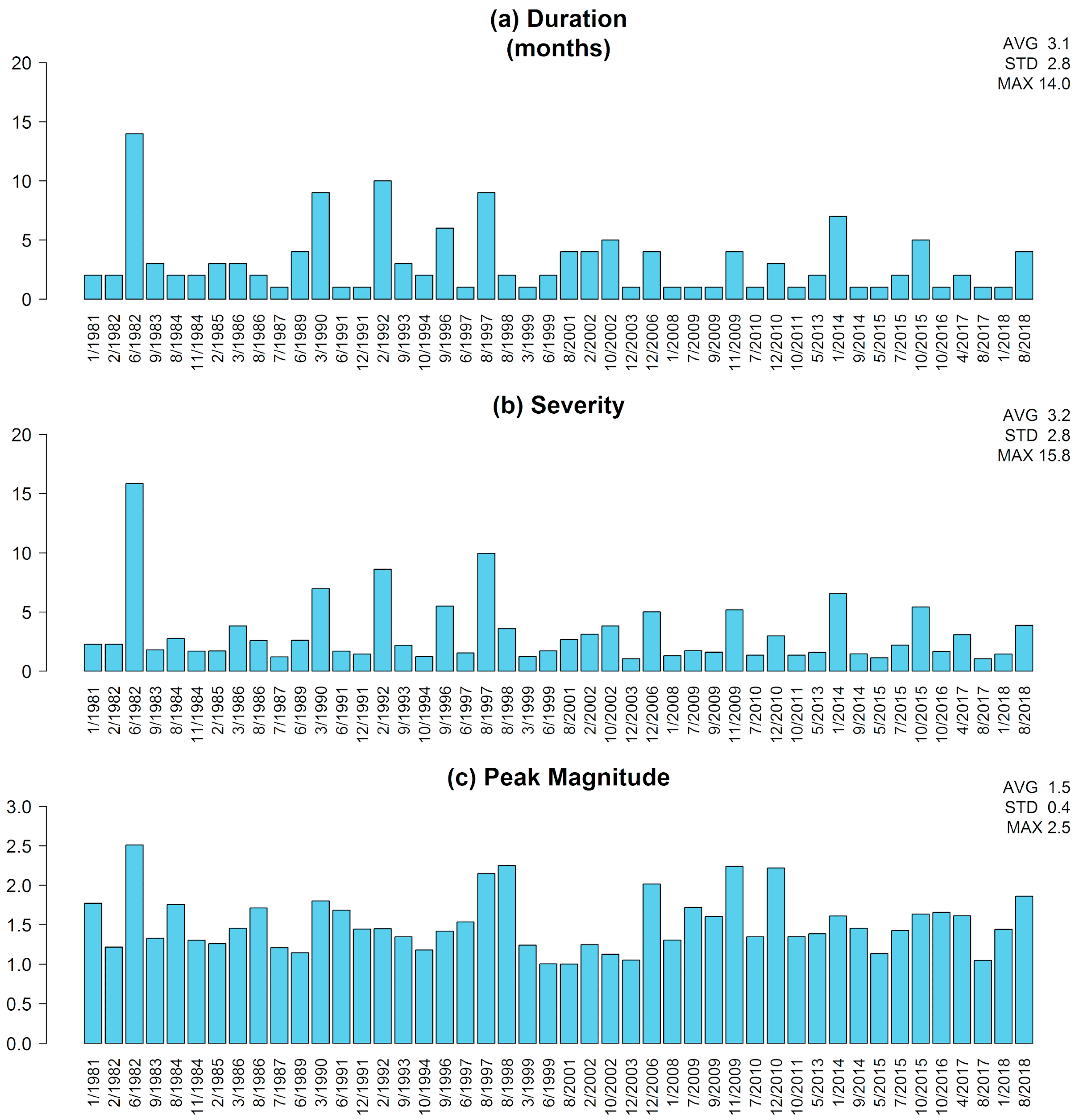
• severity is the sum of the absolute values of SPEI-1 during the event;
• duration represents the number of months;
• peak is the maximum absolute value of SPEI-i recorded during the event.

2.3. Lagrangian Approach for Atmospheric Moisture Transport Analysis

The Lagrangian analysis of atmospheric moisture transport is based on the method developed by [39,40], which utilizes the FLEXPART model [57]. In this method, the atmosphere is homogeneously divided into 3D finite elements (hereafter referred to as “parcels”) that are transported using three-dimensional wind data and stochastic convective and turbulent motions. A detailed review of the methodology for moisture transport analysis, along with its advantages and disadvantages compared to other methods, is presented by Gimeno et al. [38].

In the simulation using FLEXPART version 9.0, the global atmosphere was homogeneously divided into approximately two million parcels with constant mass. The position (latitude, longitude, and altitude) and specific humidity of each parcel were stored throughout the FLEXPART simulation. Using a post-processing program, changes in specific humidity q along the transport of each selected parcel by the winds are expressed as e − p = m(dq/dt), where m is the parcel mass and (e − p) represents the water balance in the parcel (evaporation e minus precipitation p). In this methodology, the total value of (E − P) represents the surface water balance per unit area associated with the parcels transported from the origin or to the destination of interest and results from the summation of (e − p) from all parcels located in the atmospheric column over that specific area.

Backward trajectories in time are typically used in identifying atmospheric moisture sources. According to Stohl and James [39], moisture sources are regions where the climatic water balance associated with parcels favors evapotranspiration, i.e., where (E − P) > 0. In other words, air parcels gain atmospheric moisture as they cross these source regions during their trajectories to the destination. It is important to clarify that the applied methodology does not guarantee that the atmospheric moisture absorbed by the air parcel when crossing a source will reach the destination region, as water can condense/precipitate during the journey. On the other hand, forward trajectories in time are typically used in identifying regions where the moisture balance associated with monitored parcels results in a supply of moisture to the atmosphere (E − P < 0). These regions are defined as moisture sinks (areas where precipitation or condensation exceeds evapotranspiration). In this methodology, the supply of atmospheric moisture to the destination region does not necessarily imply surface precipitation. The occurrence of surface precipitation depends on the interaction with other parcels in the air column and atmospheric dynamic conditions.

The frequency of parcel identification over the study area is daily, at 0600 UTC, and changes in specific humidity along each trajectory were calculated every 6 h (0000, 0600, 1200, and 1800 UTC). Parcel trajectories were calculated for a period of 10 days, which represents the average residence time of water vapor in the atmosphere [68]. The analysis of the average (E − P) field over the 10-day period reveals the main sources and sinks of moisture for the target region.

For this study, the main moisture sources for the LP were identified through the maxima values observed in the climatological annual mean (1980–2018) of (E − P) obtained from the backward trajectories of the parcels identified over the LP. The percentile criterion [34] was applied to define the spatial extent of the main atmospheric moisture sources. To do so, the 95th percentile of the positive E − P values obtained from the climatological annual mean of (E − P) calculated through the ten-day backward trajectories from the LP reveals the spatial location of the 5% of maximum positive values of (E − P). The spatial domain of the sources remains fixed, allowing for the evaluation of their contribution throughout the annual cycle and variations in atmospheric moisture supply during anomalous climatic events observed in the LP. It is important to note that moisture sources are not stationary [58]. While defining them on a monthly scale would provide a more accurate representation, this approach would hinder a comparative analysis of their contributions throughout the year due to the monthly variations in their spatial domains [34].

The positive values of (E − P), obtained through the 10-day backward trajectories calculated from LP were integrated over the selected sources to assess the climatology of atmospheric moisture uptake (E – P > 0) by the air parcels over each of the sources during their trajectories towards the target basin. Additionally, the negative values of (E − P), obtained through the 10-day forward trajectories calculated from the identified sources, were integrated over the target basin to obtain the climatology of atmospheric moisture supply transported by the air parcels that traveled from the sources towards the LP. Finally, the changes in these two components of moisture transport were analyzed during the anomalous climatic conditions observed in the LP.

2.4. Methods Applied in the Analysis

Simple linear regression analysis using the least squares method was conducted to investigate the potential linear impact of variations in atmospheric moisture uptake from different sources, as well as moisture supply, on climatic event indicators across the LP, following the methodology applied by Stojanovic et al. [64]. While this approach is appropriate for the aims of this paper, evaluating the combined contributions of different sources and investigating more complex relationships between variables through non-linear models could provide deeper insights into the phenomena under investigation. However, this is beyond the scope of the current paper and will be explored in future research.

The coefficient of determination (R²) was computed using the linear regression equation to gauge the extent to which changes in the moisture transport component predict variations in event duration, severity, and peak. Additionally, a Student’s t-test, set at a 95% significance level, was employed to ascertain the statistical significance of the regression coefficient.

We also applied the Mann–Kendall trend test and Sen’s slope to examine climatological trends in anomalous PRE, PET, and SPEI-1 time series, following the methodology outlined by Sorí et al. [69]. The Mann–Whitney–Wilcoxon test [70] was employed to assess the statistical significance of the disparities between indicators (duration, severity, and peak) of dry and wet events. Additionally, the Pearson and Spearman correlation coefficients were computed between PRE and PET anomalies.

Figure 2 outlines the methodology utilized in this study, consisting of two main phases: diagnosis and attribution. In the diagnosis phase, climate events were evaluated using the SPEI-1 time series. Concurrently, the atmospheric transport components linked with each source were determined via Lagrangian analysis. Subsequently, anomalies in these components were accumulated during the selected events. Finally, in the attribution phase, linear regression analysis was employed to discern any linear relationship between moisture transport variations and climate events across the LP.

3. Results and Discussions

3.1. Lagrangian Climatology of the Atmospheric Moisture Transport from the Sources to the LP

Based on the percentile criterion applied to define the spatial extent of the main atmospheric moisture sources, nine source regions were defined through the maximum positive values of the annual climatological mean of (E − P) integrated over the ten days of backward trajectories (mm/day) obtained from the LP (Figure 3a). Besides considering the LP as a local source, six of the remote sources coincide with some of the major Brazilian hydrographic basins: Amazonas (AM), Tocantins (TO), São Francisco (SF), Northeast Atlantic (NA), East/Southeast Atlantic (EA), and South Atlantic (SA). The other two are the oceanic regions east of Brazil (EBO) and south of Brazil (SBO).

Using the ERA-Interim data, the annual climatological mean of vertically integrated moisture flux (VIMF) and its respective divergence are presented in Figure 3b to aid in the visualization of moisture transport and evaporative sources and precipitating sinks from an Eulerian perspective. Over the oceans, coinciding with the regions of subtropical highs, the areas in red in Figure 3b indicate regions of maximum VIMF divergence. These areas are predominantly evaporative, acting as sources of atmospheric moisture [58,71]. The area of VIMF divergence over the Atlantic extends over the northeast of the continent, and the EA and SF basins constitute predominantly evaporative sources for the parcels that reach the LP (Figure 3a). Following the circulation associated with the South Atlantic Subtropical High, a moisture flow is observed entering the eastern continent from the Atlantic. This eastward flow progressively reduces its intensity until reaching the Amazon. Thus, although the AM, TO, and NA are considered evaporative sources for the parcels reaching the LP (Figure 3a), the blue areas indicate VIMF convergence (Figure 3b), where precipitation predominates throughout the year.

As the flow gains a northwestern component due to the presence of the Andes, it helps to deflect towards subtropical latitudes, reaching the southeast of the continent and the adjacent ocean. Over the LP, Lagrangian results indicate the basin as a local source of atmospheric moisture (Figure 3a). VIMF convergence prevails throughout the year mainly over the central-southern LP, as well as in the SA. VIMF divergence and evaporation predominate in the region of the SBO moisture source located along the southeast coast of the continent.

The importance of the LP itself, Central Brazil, Northeast Brazil, and the Atlantic as sources of atmospheric moisture for the LP has been highlighted in previous studies [28,29,30,31,33,34,37]. Variations in the source of atmospheric moisture over the oceanic area in eastern Brazil have also been observed during dry spells in the southeast of the country [49] and subtropical cyclone events in the Southwest Atlantic [50].

The annual cycle of the atmospheric moisture uptake by air parcels integrated over selected sources during their trajectories to the LP (E − P > 0, backward trajectories from LP) is presented in Figure 4. The annual cycles of PRE and PET over the LP (Figure 4a) exhibit a quite similar pattern, with maximum values in austral summer and minimums in winter. In the LP, the dry season spans from June to November when PET exceeds PRE, while the rainy season occurs from December to May when PRE surpasses PET. It is interesting to mention that the minimum and maximum peaks of moisture uptake (July and December, respectively) precede the precipitation peaks (August and January, respectively) in the LP by one month. Considering the contribution of evaporative sources to the annual total, moisture uptake predominates over the LP itself (43%) and over the AM (16%) (Figure 4c), which are the largest sources. When normalized by the area of each source, the AM ceases to be one of the main evaporative sources (contributing 4% to the annual total), while the surplus of the evaporative balances over the AS (17%) and SF (15%) sources become relevant, along with the LP (18%) (Figure 4d).

The annual cycle of atmospheric moisture supply (E − P < 0) by air parcels identified over each source into the LP (Figure 4b,e) indicates the dominant contribution of air parcels from the AM (49% of the total annual value), followed by the LP itself (25%). The supply is maximum during the austral spring months. Annual cycles of PRE over the LP and moisture supply exhibit a quite similar pattern, and the minimum peak is in August. It is important to keep in mind that the forward analysis does not guarantee that atmospheric moisture has been exclusively absorbed over the AM, as the selected parcels may absorb moisture when crossing with other sources during the trajectory to the LP. Therefore, in this case, the moisture transported by the air parcels identified over the AM could include evaporative contributions from adjacent regions, such as those located in the northeast of the continent and over the LP itself. Nonetheless, the method corroborates the relevance of moisture transport by parcels coming from the AM to the LP. When normalizing the supply by the areas of each source (Figure 4f), the importance of the TO (20% of the total value) is highlighted, along with the LP (14%) and AM (16%).

3.2. Assessment of the Anomalous Climate Events over the LP

Figure 5 presents the time series of monthly anomalies of PRE (Figure 5a) and PET (Figure 5b) integrated over the LP. The PRE anomaly series exhibits an oscillatory behavior, with maximum values in the early 1980s, as well as in the late 1990s and around 2010. Conversely, the minimums were recorded in the late 1980s and in the mid-2000s. The PET anomaly series (Figure 5b) also displays an oscillatory character, with many peaks inversely coinciding with those identified in PRE, such as the PET minimums recorded in the early 1980s and late 1990s. The Pearson and Spearman correlation coefficients between PRE and PET anomalies time series show similar negative values, around 0.4 (significant at 95%), indicating that as PRE increases (decreases), PET decreases (increases). Both linear trend and Mann–Kendall tests detected a significant increasing trend at 99.99% only in the PET anomaly time series (Figure 5b), indicating the trend of increasing potential evapotranspiration in the basin over the last 40 years.

From these time series, we calculate the SPEI-1 (Figure 5c). In general, dry conditions prevailed during La Niña events (such as 1988/89, 1999/2000, 2007), while wet conditions were observed during El Niño events (e.g., 1982/83, 1991/92, 1997/98, 2015), aligning with previous studies [72]. While not the primary objective of this paper, the analysis of the modulation of anomalous conditions over the La Plata Basin and the moisture transport by the El Niño Southern Oscillation phenomenon could enhance our understanding of the region’s climate variability and will be the subject of future research.

Agreeing with the observations in PRE and PET, there is a predominance of wet periods in the 1980s and 1990s, followed by a prevalence of dry periods from 2000 to 2018. The Mann–Kendall trend test and Sen’s slope detect a statistically significant decreasing trend in the SPEI-1 time series (slope: −0.0008) at a confidence level of 99.9%. The observed statistically significant decreasing trend in the SPEI-1 time series, combined with the noted trend of increasing evapotranspiration alongside stable precipitation levels, provides valuable insight into the prevailing dry periods observed after the 2000s.

Applying the criteria explained in detail in Section 2.2 to the SPEI-1 time series shown in Figure 5c revealed 49 dry events and 46 wet events. Figure 6 and Figure 7 list the dry and wet events (each bar represents a climate event), respectively, and the indicators associated, as well as the average, standard deviation, and the maxima values. The average duration of 3 months and the average severity of 3.2 were found to be similar for both dry and wet events. However, upon examining the standard deviation values illustrated in Figure 6a,b, it becomes evident that dry events exhibit lower variability in both duration and severity, with values of 2.2 months and 2.3, respectively, compared to wet events, which show higher variability, with values of 2.8 months for duration and 2.8 for severity (Figure 7a,b). Additionally, wet events present higher maxima in both duration (14 months) and severity (15.8), registered during the event of 1982, compared to dry events (10 months and 11.8, respectively; verified during the event of 1988). The average absolute peak value of 1.5 in both cases corresponds to severe conditions, with a deviation of 0.3 for dry events and 0.4 for wet events. Notably, the maximum peak of 2.5 observed during the wet event of 1982 slightly surpasses the peak of 2.4 recorded during the dry event of 2008, both reaching the extreme category. Importantly, the Wilcoxon test, conducted at a 95% confidence level, indicated no statistically significant difference between the duration, severity, and peak of dry and wet events.

3.3. Variations in Moisture Transport from the Sources during the Anomalous Climate Events in the LP

Simple linear regression analysis was conducted to assess whether variations in the moisture transport from different sources would affect the indicators associated with anomalous climate events in the LP. The coefficient of determination (R²) was calculated using the linear regression equation, representing the proportion of variance in the dependent variable (severity, duration, and peak of events) predictable with respect to the independent variable (source contribution). The statistical significance of the regression coefficient was evaluated using the t-Student test. The results are presented in

Table 1. Slope, intercept and coefficient of determination (R²) for duration, severity, and peak magnitude values with respect to anomalies of moisture uptake and supply associated with the sources and accumulated during the dry and wet events across the LP. The highlighted slope values have a statistically significant linear relationship with the respective moisture transport anomalies, considering the confidence intervals of * 95%, ** 99%, and *** 99.9%.

		Duration			Severity			Peak Magnitude
	Sources	Slope	Intercept	R2	Slope	Intercept	R2	Slope	Intercept	R2
Uptake Dry events	AM	−0.034 ***	2.282	0.314	−0.036 ***	2.365	0.311	−0.003 *	1.485	0.092
	NA	−0.125 ***	2.280	0.342	−0.166 ***	2.139	0.572	−0.012 **	1.481	0.118
	EBO	−0.031	2.660	0.055	−0.046 **	2.588	0.133	−0.008 ***	1.452	0.211
	EA	−0.04	2.946	0.013	−0.071	2.985	0.017	−0.020 **	1.503	0.133
	SF	−0.038	2.777	0.052	−0.065 **	2.698	0.177	−0.011 ***	1.474	0.261
	TO	−0.091 **	2.515	0.004	−0.135 ***	2.369	0.328	−0.020 ***	1.438	0.333
	SBO	0.003	3.024	0.001	0.005	3.115	0.003	0.002	1.536	0.008
	SA	0.113	2.878	0.001	0.239 *	2.806	0.072	0.036 *	1.500	0.080
	LP	0.014 *	2.583	0.077	0.019 **	2.518	0.153	0.002 *	1.479	0.087
Supply Dry events	AM	−0.013 ***	1.509	0.469	−0.014 ***	1.412	0.563	−0.001 **	1.426	0.125
	NA	−0.078 ***	1.878	0.438	−0.091 ***	1.789	0.561	−0.006 *	1.459	0.108
	EBO	−0.055 *	2.372	0.111	−0.060 **	2.422	0.123	−0.007 *	1.463	0.082
	EA	−0.044	2.885	0.013	−0.038	3.017	0.009	−0.004	1.538	0.004
	SF	−0.098 **	2.338	0.137	−0.098 **	2.449	0.125	−0.008	1.491	0.031
	TO	−0.086 ***	1.960	0.257	−0.098 ***	1.919	0.313	−0.009 *	1.441	0.108
	SBO	−0.010	3.037	0.002	0.002	3.152	0.000	0.002	1.552	0.003
	SA	−0.041	3.023	0.001	0.077	3.184	0.003	0.011	1.556	0.003
	LP	−0.024 ***	1.707	0.306	−0.026 ***	1.737	0.319	−0.002 *	1.446	0.071
Uptake Wet events	AM	0.025 ***	2.515	0.345	0.029 ***	2.476	0.486	0.002 **	1.461	0.172
	NA	0.136 ***	2.040	0.440	0.142 ***	2.054	0.484	0.010 **	1.433	0.145
	EBO	0.052 **	2.567	0.179	0.047 **	2.675	0.144	0.003	1.483	0.021
	EA	0.003	3.082	0.000	−0.012	3.167	0.002	0.004	1.508	0.008
	SF	0.068 **	2.661	0.116	0.060 *	2.775	0.084	0.005	1.485	0.016
	TO	0.130 ***	2.313	0.320	0.126 ***	2.398	0.301	0.005	1.482	0.013
	SBO	−0.035 *	2.859	0.064	−0.019	3.023	0.003	0.001	1.520	0.004
	SA	−0.221	2.884	0.010	−0.063	3.089	0.003	0.012	1.526	0.006
	LP	−0.039 ***	1.861	0.361	−0.042 ***	1.811	0.436	−0.004 ***	1.372	0.288
Supply Wet events	AM	0.010 ***	1.815	0.480	0.012 ***	1.686	0.646	0.001 ***	1.383	0.300
	NA	0.068 ***	1.720	0.632	0.074 ***	1.648	0.771	0.006 ***	1.399	0.258
	EBO	0.072 ***	2.105	0.293	0.068 ***	2.211	0.267	0.005 *	1.447	0.066
	EA	0.113	2.633	0.058	0.081	2.821	0.019	0.002	1.507	0.001
	SF	0.163 ***	1.626	0.569	0.156 ***	1.750	0.522	0.009 *	1.436	0.079
	TO	0.114 ***	1.304	0.782	0.115 ***	1.338	0.813	0.008 ***	1.388	0.220
	SBO	−0.096 **	3.231	0.123	−0.090 *	3.281	0.105	−0.001	1.516	0.001
	SA	−0.307	3.205	0.012	−0.315	3.267	0.014	0.014	1.509	0.004
	LP	0.026 ***	1.526	0.371	0.027 ***	1.523	0.407	0.003 ***	1.348	0.247

, and the analysis of the results highlights the linear relationships with respect to dry and wet events, associated with significant regression coefficients at a confidence interval of 99.9% and R² values around 0.3 or larger. R² values above 0.5–0.6 are generally considered strong in climate studies with highly variable factors like precipitation, but lower values around 0.3 may still be reasonable [73].

There is a significant linear relationship between the duration of dry and wet climate events and variations in the uptake and supply of atmospheric moisture associated with the AM and NA sources. For these cases, R² values obtained vary from 0.314 for the uptake of moisture associated with the AM during dry events to 0.632 for the supply of moisture associated with NA during wet events. This implies that longer dry (wet) events were associated with a higher decrease (increase) in uptake and supply of atmospheric moisture associated with both basins.

It is also noteworthy a linear relationship between the severity of dry and wet climatic events and variations in both the uptake and supply of atmospheric moisture associated with the AM, NA, and TO basins. For these cases, R² values obtained vary from 0.301 for the uptake of moisture associated with the TO during wet events to 0.813 for the supply of moisture associated also with the TO during wet events. More severe dry (wet) events were associated with a higher decrease (increase) in uptake and supply of atmospheric moisture associated with these basins located northwards.

Besides the role of the AM, NA, and TO basins, a higher increase in the moisture supply from the SF (with R² values around 0.5) and EBO (with R² values around 0.3) also contribute to both the duration and severity of wet events. According to Leyba et al. [37], although the contribution from the Southwest Atlantic is climatologically small for the southeastern continent, its importance increases during precipitation events. The highest R² values (exceeding 0.5) were obtained for the positive relationship between the duration/severity of wet events and the moisture supply anomalies from the AM, NA, SF, and TO basins. In fact, the R² values for the TO reached 0.8.

In terms of peak, the relationships obtained differ from dry to wet climate events, and the R² values are around 0.3. On one hand, higher peak drought was associated with higher decrease in moisture uptake over the TO, SF and EBO sources, i.e., with uptake over eastern regions. On the other hand, higher peak wet events were associated with a higher increase in moisture supply from the northern AM, NA, and TO basins.

4. Summary and Conclusions

The general aim of this diagnostic and attribution paper is to apply simple linear regression analysis to examine the linear relationship between the duration, severity, and peak of anomalous climate events in the La Plata Basin (LP) from 1980 to 2018 and variations in atmospheric moisture transport from major sources, using a Lagrangian approach.

A total of 49 events of meteorological drought and 46 wet events have been identified over the LP and characterized through the standardized precipitation evapotranspiration index time series accumulated for one month (SPEI-1), as proposed by McKee et al. [21]. While dry and wet events showed similar average durations and severities, dry events exhibited lower variability according to the standard deviation values. Wet events had higher variability and maximum values, notably for the extreme event of 1982. However, no statistically significant difference was found between dry and wet events in terms of duration, severity, and peak values.

For the identified dry and wet events, the Lagrangian analysis computed changes in the uptake over the major atmospheric moisture sources identified for the LP, as well as in the supply of atmospheric moisture from these sources to the basin. Monthly anomalies in these moisture transport components were calculated and subsequently accumulated during each extreme climate event.

Under a climatological perspective, the Amazonas basin (AM) is the major remote moisture source in absolute values. When taking into account the source area, the basins such as the South Atlantic (SA), Tocantins (TO), and São Francisco (SF) become relevant.

A simple linear regression analysis was then conducted to evaluate the relationship between the indicators (duration, severity, and peak) characterizing the anomalous climate events over the LP and the variations in atmospheric moisture transport associated with the sources considered. The main findings are summarized in Figure 8, which highlights the results obtained with a 99.9% confidence interval. The main conclusions are:

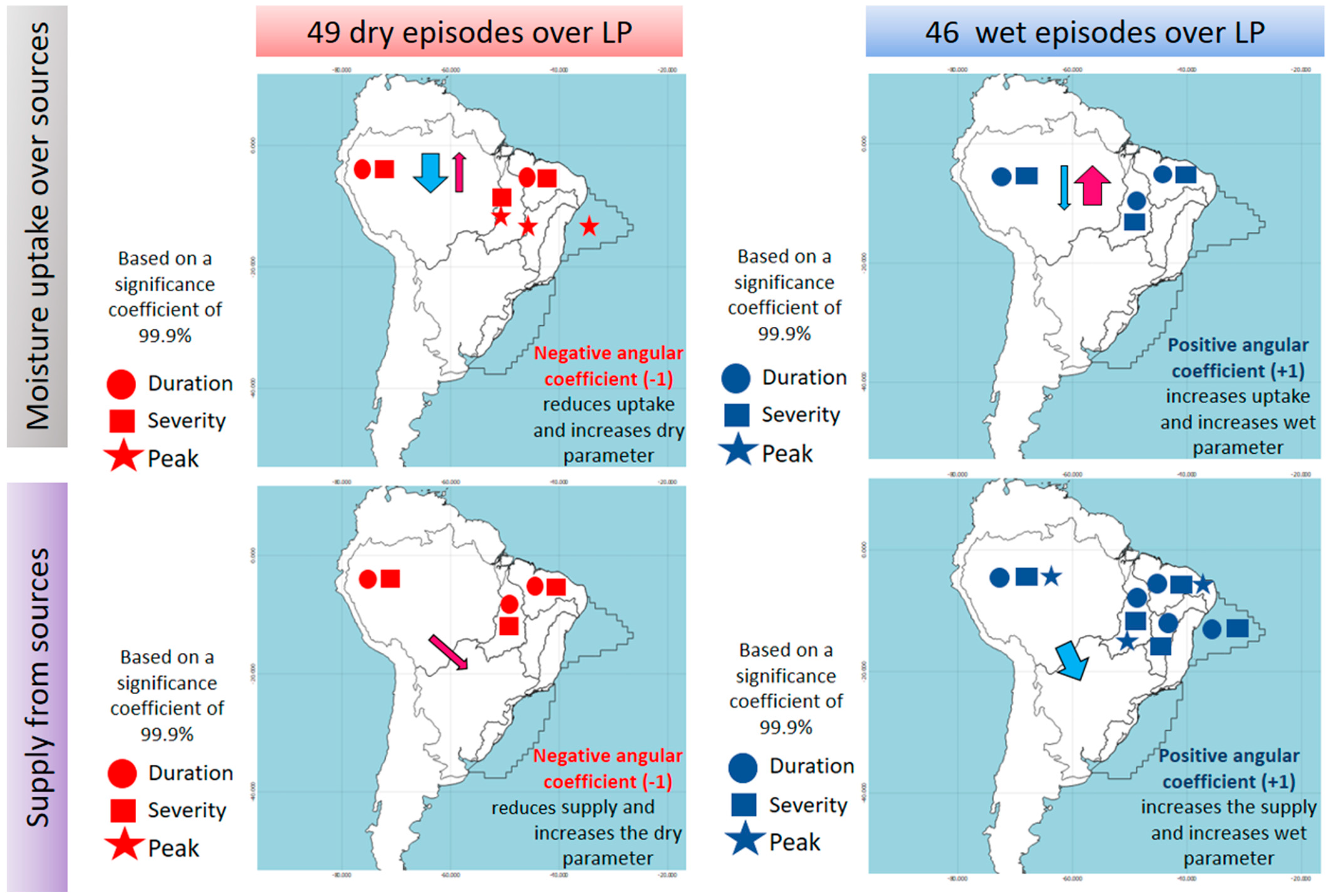
• Moisture Transport and Event Severity: The moisture transport (uptake and supply) from the AM, North Atlantic (NA), and TO basins influences the severity of anomalous climate events over the LP, highlighting the importance of transport from northern latitudes to subtropical areas;
• Duration of Anomalous Climate events: There is a relationship between the duration of anomalous climate events and variations in the uptake and supply of atmospheric moisture associated with the NA and AM sources;
• Contribution of the Moisture Supply from Other Regions: Besides the NA, AM, and TO basins, a higher increase in moisture supply from the SF region and the oceanic area east of Brazil (EBO) also contributes to both the duration and severity of wet events;
• Peaks of Wet and Dry events: Higher peak wet events are associated with a significant increase in moisture supply from the northern NA, AM, and TO basins, while higher peak droughts are associated with a significant decrease in moisture uptake over the TO, SF, and EBO regions, which are sources located east of the continent.

It is worth noting that this study primarily focused on exploring the potential for a linear relationship between climate events over the LP and moisture transport of various sources via simple linear regression analysis. While this approach is appropriate for our objectives, it is worth considering the potential benefits of exploring non-linear models for a more accurate depiction of the relationships, especially for predictive purposes. Additionally, assessing the combined contributions of different sources could provide a more comprehensive understanding of the phenomena under investigation. Investigating the underlying physical mechanisms responsible for anomalous patterns was not within the scope of this research. Additionally, while our study centered on the LP, it is crucial to recognize the distinct spatial and temporal characteristics inherent to each climatic event. In a future work, accounting for intra-basins variability would enrich the spatial-temporal analysis of individual cases, leading to a more comprehensive understanding of the moisture transport during anomalous climate events in South America.

The results reflect the observed climate variations during the period 1980–2018. In future climate scenarios, climatic conditions, circulation patterns, and atmospheric moisture transport between remote regions and the LP may change. Projections based on IPCC scenarios indicate an increase in rainfall volume and in the frequency of extreme daily events in the LP [74]. Local evapotranspiration will be a significant driver for precipitation in the LP, along with moisture transport from the southwestern Atlantic [75]. Therefore, further investigation applying this Lagrangian approach in future climate scenarios would be valuable for understanding the impacts of climate change on the water balance.

Our findings elucidate the sensitivity of the LP to variations in the water balance in distant regions through atmospheric moisture transport. Any alteration in the climate system at the moisture source can have significant adverse effects on the LP, including impacts on biodiversity, society, economic activities, and water supply. These results underscore the importance of recognizing the interconnectedness between different regions when developing adaptive strategies to mitigate the potential negative consequences of climate change on the LP.

References

1. Masson-Delmotte, V.; Zhai, P.; Pirani, A.; Connors, S.L.; Péan, C.; Berger, S.; Caud, N.; Chen, Y.; Goldfarb, L.; Gomis, M.I. (Eds.) IPCC, 2021. Climate Change 2021: The Physical Science Basis. Contribution of Working Group I to the Sixth Assessment Report of the Intergovernmental Panel on Climate Change; Cambridge University Press: Cambridge, UK; New York, NY, USA, 2023; p. 2391. [Google Scholar] [CrossRef]
2. Cunha, A.P.M.A.; Zeri, M.; Deusdará Leal, K.; Costa, L.; Cuartas, L.A.; Marengo, J.A.; Tomasella, J.; Vieira, R.M.; Barbosa, A.A.; Cunningham, C.; et al. Extreme Drought Events over Brazil from 2011 to 2019. Atmosphere 2019, 10, 642. [Google Scholar] [CrossRef]
3. Drumond, A.; Stojanovic, M.; Nieto, R.; Gimeno, L.; Liberato, M.L.R.; Pauliquevis, T.; Oliveira, M.; Ambrizzi, T. Dry and Wet Climate Periods over Eastern South America: Identification and Characterization through the SPEI Index. Atmosphere 2021, 12, 155. [Google Scholar] [CrossRef]
4. Naumann, G.; Podesta, G.; Marengo, J.; Luterbacher, J.; Bavera, D.; Arias Muñoz, C.; Barbosa, P.; Cammalleri, C.; Chamorro, L.; Cuartas, L.A.; et al. The 2019–2021 Extreme Drought Episode in La Plata Basin; Publications Office of the European Union: Luxembourg, 2021; ISBN 978-92-76-41898-6. [Google Scholar] [CrossRef]
5. Marengo, J.A.; Cunha, A.P.; Cuartas, L.A.; Leal, K.R.D.; Broedel, E.; Seluchi, M.E.; Michelin, C.M.; De Praga Baião, C.F.; Angulo, E.C.; Almeida, E.K.; et al. Extreme drought in the Brazilian Pantanal in 2019–2020: Characterization, causes, and impacts. Front. Water 2021, 3, 639204. [Google Scholar] [CrossRef]
6. Fortunato de Faria, L.; Reboita, M.S.; Mattos, E.V.; Carvalho, V.S.B.; Martins Ribeiro, J.G.; Capucin, B.C.; Drumond, A.; Paes dos Santos, A.P. Synoptic and Mesoscale Analysis of a Severe Weather Event in Southern Brazil at the End of June 2020. Atmosphere 2023, 14, 486. [Google Scholar] [CrossRef]
7. Bartolomei, F.; Reboita, M.S.; da Rocha, R.P. Ciclones extratropicais causadores de eventos extremos no sul do Brasil no inverno de 2023. Terrae Didat. 2024, 20, e024003. [Google Scholar] [CrossRef]
8. CNN 2024. Available online: https://edition.cnn.com/2024/05/03/weather/brazil-rain-floods-intl/index.html (accessed on 17 May 2024).
9. Barros, V.; Clarke, R.; Dias, P.S. (Eds.) Climate Change in the La Plata Basin; Inter-American Institute for Global Change Research: São José dos Campos, Brazil, 2006; p. 219. Available online: https://www2.atmos.umd.edu/~berbery/lpb/climate_change_lpb.pdf (accessed on 17 May 2024).
10. Cavalcanti, I.; Carril, A.; Penalba, O.; Grimm, A.; Menéndez, C.; Sanchez, E.; Cherchi, A.; Sörensson, A.; Robledo, F.; Rivera, J.; et al. Flach Precipitation extremes over La Plata Basin—Review and new results from observations and climate simulations. J. Hydrol. 2015, 523, 211–230. [Google Scholar] [CrossRef]
11. Barros, V.; Chamorro, L.; Coronel, G.; Baez, J. The major discharge events in the Paraguay River: Magnitudes, source regions, and climate forcings. J. Hydrometeorol. 2004, 5, 1161–1170. [Google Scholar] [CrossRef]
12. Barros, V.R.; Boninsegna, J.A.; Camilloni, I.A.; Chidiak, M.; Magrín, G.O.; Rusticucci, M. Climate change in Argentina: Trends, projections, impacts and adaptation. Wiley Interdiscip. Rev. Clim. Chang. 2015, 6, 151–169. [Google Scholar] [CrossRef]
13. de Freitas, A.A.; Reboita, M.S.; Carvalho, V.S.B.; Drumond, A.; Ferraz, S.E.T.; da Silva, B.C.; da Rocha, R.P. Atmospheric and Oceanic Patterns Associated with Extreme Drought Events over the Paraná Hydrographic Region, Brazil. Climate 2023, 11, 12. [Google Scholar] [CrossRef]
14. Seneviratne, S.; Nicholls, N.; Easterling, D.; Goodess, C.; Kanae, S.; Kossin, J.; Luo, Y.; Marengo, J.; McInnes, K.; Rahimi, M.; et al. Changes in Climate Extremes and Their Impacts on the Natural Physical Environment: An Overview of the IPCC SREX report. Clim. Chang. 2012, 109, 1–4. Available online: https://www.ipcc.ch/site/assets/uploads/2018/03/SREX-Chap3_FINAL-1.pdf (accessed on 17 May 2024).
15. Lloyd-Hughes, B. The impracticality of a universal drought definition. Theor. Appl. Climatol. 2014, 117, 607–611. [Google Scholar] [CrossRef]
16. Wilhite, D.A.; Glantz, M.H. Understanding the drought phenomenon: The role of definitions. Water Int. 1985, 10, 111–120. [Google Scholar] [CrossRef]
17. Redmond, K.T. The depiction of drought: A commentary. Bull. Am. Meteorol. Soc. 2002, 83, 1143–1147. [Google Scholar] [CrossRef]
18. WMO. Standardized Precipitation Index User Guide; WMO-1090: Geneva, Switzerland, 2012; p. 24. Available online: https://library.wmo.int/idurl/4/39629 (accessed on 28 June 2024).
19. Hanel, M.; Rakovec, O.; Markonis, Y.; Máca, P.; Samaniego, L.; Kyselý, J.; Kumar, R. Revisiting the recent European droughts from a long-term perspective. Sci. Rep. 2018, 8, 9499. [Google Scholar] [CrossRef]
20. Spinoni, J.; Naumann, G.; Carrao, H.; Barbosa, P.; Vogt, J. World drought frequency, duration, and severity for 1951–2010. Int. J. Climatol. 2014, 34, 2792–2804. [Google Scholar] [CrossRef]
21. McKee, T.B.; Doesken, N.J.; Kleist, J. The relationship of drought frequency and duration to time scales. In Proceedings of the Eighth Conference on Applied Climatology, Boston, MA, USA, 17–22 January 1993; pp. 179–184. Available online: https://www.droughtmanagement.info/literature/AMS_Relationship_Drought_Frequency_Duration_Time_Scales_1993.pdf (accessed on 17 May 2024).
22. Hayes, M.; Svodoba, M.; Wall, N.; Widhalm, M. The Lincoln Declaration on Drought Indices: Universal meteorological drought index recommended. Bull. Am. Meteorol. Soc. 2011, 92, 485–488. [Google Scholar] [CrossRef]
23. Vicente-Serrano, S.M.; Begueria, S.; Lopez-Moreno, J.I. A multiscalar drought index sensitive to global warming: The Standardized Precipitation Evapotranspiration Index. J. Clim. 2010, 23, 1696–1718. [Google Scholar] [CrossRef]
24. Vicente-Serrano, S.M.; Beguería, S.; Lorenzo-Lacruz, J.; Camarero, J.J.; López-Moreno, J.I.; Azorin-Molina, C.; Revuelto, J.; Morán-Tejeda, E.; Sanchez-Lorenzo, A. Performance of Drought Indices for Ecological, Agricultural and Hydrological Applications. Earth Interact. 2012, 16, 1–27. [Google Scholar] [CrossRef]
25. Gurrapu, S.; Chipanshi, A.; Sauchyn, D.; Howard, A. Comparison of the SPI and SPEI on predicting drought conditions and streamflow in the Canadian prairies. In Proceedings of the 28th Conference on Hydrology, Atlanta, GA, USA, 2–6 February 2014; pp. 2–6. Available online: https://ams.confex.com/ams/94Annual/webprogram/Paper241519.html (accessed on 28 June 2024).
26. Sordo-Ward, A.; Bejarano, M.D.; Iglesias, A.; Asenjo, V.; Garrote, L. Analysis of Current and Future SPEI Droughts in the La Plata Basin Based on Results from the Regional Eta Climate Model. Water 2017, 9, 857. [Google Scholar] [CrossRef]
27. Mendiola, M.E.P.; Blázquez, J.; Solman, S.A. Characterization of wet and dry periods over southern South America. In Climate Dynamics; Springer: Berlin/Heidelberg, Germany, 2024. [Google Scholar] [CrossRef]
28. Drumond, A.; Nieto, R.; Gimeno, L.; Ambrizzi, T. A Lagrangian identification of major sources of moisture over central Brazil and La Plata Basin. J. Geophys. Res. 2008, 113, D14128. [Google Scholar] [CrossRef]
29. Arraut, J.M.; Nobre, C.; Barbosa, H.M.J.; Obregon, G.; Marengo, J. Aerial rivers and lakes: Looking at large-scale moisture transport and its relation to Amazonia and to subtropical rainfall in South America. J. Clim. 2012, 25, 543–556. [Google Scholar] [CrossRef]
30. Nieto, R.; Castillo, R.; Drumond, A. The modulation of oceanic moisture transport by the hemispheric annular modes. Front. Earth Sci. 2014, 2, 11. [Google Scholar] [CrossRef]
31. Martinez, J.A.; Dominguez, F. Sources of atmospheric moisture for the La Plata River basin. J. Clim. 2014, 27, 6737–6753. [Google Scholar] [CrossRef]
32. Drumond, A.; Marengo, J.; Ambrizzi, A.; Nieto, R.; Moreira, L.; Gimeno, L. The role of the Amazon Basin moisture in the atmospheric branch of the hydrological cycle: A Lagrangian analysis. Hydrol. Earth Syst. Sci. 2014, 18, 2577–2598. [Google Scholar] [CrossRef]
33. Moura, L.Z.; Lima, C.H.R. Analysis of atmospheric moisture transport to the Upper Paraná River basin. Int. J. Climatol. 2018, 38, 5153–5167. [Google Scholar] [CrossRef]
34. Drumond, A.; Stojanovic, M.; Nieto, R.; Vicente-Serrano, S.M.; Gimeno, L. Linking anomalous moisture transport and drought episodes in the IPCC reference regions. Bull. Am. Meteorol. Soc. 2019, 100, 1481–1498. [Google Scholar] [CrossRef]
35. Lemes, M.d.C.R.; de Oliveira, G.S.; Fisch, G.; Tedeschi, R.G.; da Silva, J.P.R. Analysis of moisture transport from Amazonia to Southeastern Brazil during the austral summer. Rev. Bras. Geogr. Física 2020, 13, 2650–2670. [Google Scholar] [CrossRef]
36. Zanin, P.R.; Satyamurty, P. Hydrological processes interconnecting the two largest watersheds of South America from seasonal to intra-monthly time scales: A critical review. Int. J. Climatol. 2020, 40, 3971–4005. [Google Scholar] [CrossRef]
37. Leyba, I.M.; Solman, S.A.; Saraceno, M.; Martinez, J.A.; Dominguez, F. The South Atlantic Ocean as a moisture source region and its relation with precipitation in South America. Clim. Dyn. 2023, 61, 1741–1756. [Google Scholar] [CrossRef]
38. Gimeno, L.; Vázquez, M.; Eiras-Barca, J.; Sorí, R.; Stojanovic, M.; Algarra, I.; Nieto, R.; Ramos, A.M.; Durán-Quesada, A.M.; Dominguez, F. Recent progress on the sources of continental precipitation as revealed by moisture transport analysis. Earth Sci. Rev. 2020, 201, 103070. [Google Scholar] [CrossRef]
39. Stohl, A.; James, P. A Lagrangian Analysis of the Atmospheric Branch of the Global Water Cycle. Part I: Method Description, Validation, and Demonstration for the August 2002 Flooding in Central Europe. J. Hydrometeorol. 2004, 5, 656–678. [Google Scholar] [CrossRef]
40. Stohl, A.; James, P. A Lagrangian analysis of the atmospheric branch of the global water cycle: Part II: Moisture Transports between Earth’s Ocean Basins and River Catchments. J. Hydrometeorol. 2005, 6, 961–984. [Google Scholar] [CrossRef]
41. Dirmeyer, P.A.; Brubaker, K.L. Characterization of the global hydrologic cycle from a back-trajectory analysis of atmospheric water vapor. J. Hydrometeorol. 2007, 8, 20–37. [Google Scholar] [CrossRef]
42. Sodemann, H.; Zubler, E. Seasonal and inter-annual variability of the moisture sources for Alpine precipitation during 1995–2002. Int. J. Climatol. 2010, 30, 947–961. [Google Scholar] [CrossRef]
43. Knippertz, P.; Wernli, H.; Gläser, G. A Global Climatology of Tropical Moisture Exports. J. Clim. 2013, 26, 3031–3045. [Google Scholar] [CrossRef]
44. Drumond, A.; Nieto, R.; Gimeno, L.; Trigo, R.M.; Ambrizzi, T.; De Souza, E. A Lagrangian Identification of the Main Sources of Moisture Affecting Northeastern Brazil during Its Pre-Rainy and Rainy Seasons. PLoS ONE 2010, 5, e11205. [Google Scholar] [CrossRef]
45. Sorí, R.; Marengo, J.A.; Nieto, R.; Drumond, A.; Gimeno, L. The Atmospheric Branch of the Hydrological Cycle over the Negro and Madeira River Basins in the Amazon Region. Water 2018, 10, 738. [Google Scholar] [CrossRef]
46. Hoyos, I.; Dominguez, F.; Cañón-Barriga, J.; Martínez, J.A.; Nieto, R.; Gimeno, L.; Dirmeyer, P.A. Moisture origin and transport processes in Colombia, northern South America. Clim. Dyn. 2018, 50, 971–990. [Google Scholar] [CrossRef]
47. Nieto, R.; Gallego, D.; Trigo, R.M.; Ribera, P.; Gimeno, L. Dynamic identification of moisture sources in the Orinoco basin in equatorial South America. Hydrol. Sci. J. 2008, 53, 602–617. [Google Scholar] [CrossRef]
48. Braz, D.F.; Ambrizzi, T.; Da Rocha, R.P.; Algarra, I.; Nieto, R.; Gimeno, L. Assessing the moisture transports associated with nocturnal low-level jets in continental South America. Front. Environ. Sci. 2021, 9, 657764. [Google Scholar] [CrossRef]
49. Pampuch, L.A.; Drumond, A.; Gimeno, L.; Ambrizzi, T. Anomalous patterns of SST and moisture sources in the South Atlantic Ocean associated with dry events in southeastern Brazil. Int. J. Climatol. 2016, 36, 4913–4928. [Google Scholar] [CrossRef]
50. Gozzo, L.F.; da Rocha, R.P.; Gimeno, L.; Drumond, A. Climatology and numerical case study of moisture sources associated with subtropical cyclogenesis over the southwestern Atlantic Ocean. J. Geophys. Res. Atmos. 2017, 122, 5636–5653. [Google Scholar] [CrossRef]
51. Pérez-Alarcón, A.; Coll-Hidalgo, P.; Fernández-Álvarez, J.C.; Sorí, R.; da Rocha, R.P.; Simões Reboita, M.; Nieto, R.; Gimeno, L. Quantifying the related precipitation and moisture sources in the lifecycle of subtropical cyclones in the South Atlantic basin. In Quarterly Journal of the Royal Meteorological Society; Royal Meteorological Society (RMetS): London, UK, 2024. [Google Scholar] [CrossRef]
52. Harris, I.; Osborn, T.J.; Jones, P.; Lister, D. Version 4 of the CRU TS monthly high-resolution gridded multivariate climate dataset. Sci. Data 2020, 7, 109. [Google Scholar] [CrossRef] [PubMed]
53. Allen, R.G.; Pereira, L.S.; Raes, D.; Smith, M. Crop Evapotranspiration—Guidelines for Computing Crop Water Requirements; FAO Irrigation and Drainage Paper No. 56; Food and Agriculture Organization of the United Nations: Rome, Italy, 1998. [Google Scholar]
54. National Center for Atmospheric Research Staff. The Climate Data Guide: CRU TS Gridded Precipitation and Other Meteorological Variables Since 1901. Available online: https://climatedataguide.ucar.edu/climate-data/cru-ts-gridded-precipitation-and-other-meteorological-variables-1901 (accessed on 17 May 2024).
55. Carvalho, L.M. Assessing precipitation trends in the Americas with historical data: A review. Wiley Interdiscip. Rev. Clim. Chang. 2020, 11, e627. [Google Scholar] [CrossRef]
56. Dee, D.P.; Uppala, S.M.; Simmons, A.J.; Berrisford, P.; Poli, P.; Kobayashi, S.; Andrae, U.; Balmaseda, M.A.; Balsamo, G.; Bauer, P.; et al. The ERA-Interim reanalysis: Configuration and performance of the data assimilation system. Q. J. R. Meteorol. Soc. 2001, 137, 553–597. [Google Scholar] [CrossRef]
57. Stohl, A.; Forster, C.; Frank, A.; Seibert, P.; Wotawa, G. Technical note: The Lagrangian particle dispersion model FLEXPART version 6.2. Atmos. Chem. Phys. 2005, 5, 2461–2474. [Google Scholar] [CrossRef]
58. Gimeno, L.; Nieto, R.; Drumond, A.; Castillo, R.; Trigo, R.M. Influence of the intensification of the major oceanic moisture sources on continental precipitation. Geophys. Res. Lett. 2013, 40, 1443–1450. [Google Scholar] [CrossRef]
59. Montini, T.L.; Jones, C.; Carvalho, L.M.V. The South American low-level jet: A new climatology, variability, and changes. J. Geophys. Res. Atmos. 2019, 124, 1200–1218. [Google Scholar] [CrossRef]
60. GRDC. WMO Basins and Sub-Basins/Global Runoff Data Centre, GRDC, 3rd, rev. ext. ed.; Federal Institute of Hydrology (BfG): Koblenz, Germany, 2020. [Google Scholar]
61. Beguería, S.; Vicente-Serrano, S.M.; Reig, F.; Latorre, B. Standardized Precipitation Evapotranspiration Index (SPEI) revisited: Parameter fitting, evapotranspiration models, tools, datasets and drought monitoring. Int. J. Climatol. 2014, 34, 3001–3023. [Google Scholar] [CrossRef]
62. Vicente-Serrano, S.M.; Beguería, S. Short communication comment on “candidate distributions for climatological drought indices (SPI and SPEI)” by James, H. Stagge et al. Int. J. Climatol. 2016, 36, 2120–2131. [Google Scholar] [CrossRef]
63. Liu, Z.; Lu, G.; He, H.; Wu, Z.; He, J. Anomalous Features of Water Vapor Transport during Severe Summer and Early Fall Droughts in Southwest China. Water 2017, 9, 244. [Google Scholar] [CrossRef]
64. Stojanovic, M.; Drumond, A.; Nieto, R.; Gimeno, L. Variations in Moisture Supply from the Mediterranean Sea during Meteorological Drought Episodes over Central Europe. Atmosphere 2018, 9, 278. [Google Scholar] [CrossRef]
65. Stojanovic, M.; Drumond, A.; Nieto, R.; Gimeno, L. Moisture Transport Anomalies over the Danube River Basin during Two Drought Events: A Lagrangian Analysis. Atmosphere 2017, 8, 193. [Google Scholar] [CrossRef]
66. Salah, Z.; Nieto, R.; Drumond, A.; Gimeno, L.; Vicente-Serrano, S. A Lagrangian analysis of the moisture budget over the Fertile Crescent during two intense drought events. J. Hydrol. 2018, 560, 382–395. [Google Scholar] [CrossRef]
67. Drumond, A.; Nieto, R.; Gimeno, L. A Lagrangian approach for investigating anomalies in the moisture transport during drought events. Cuad. Investig. Geográfica 2016, 42, 113–125. [Google Scholar] [CrossRef]
68. Numaguti, A. Origin and recycling processes of precipitating water over the Eurasian continent: Experiments using an atmospheric general circulation model. J. Geophys. Res. Atmos. 1999, 104, 1957–1972. [Google Scholar] [CrossRef]
69. Sorí, R.; Vázquez, M.; Stojanovic, M.; Nieto, R.; Liberato, M.L.R.; Gimeno, L. Hydrometeorological droughts in the Miño–Limia–Sil hydrographic demarcation (northwestern Iberian Peninsula): The role of atmospheric drivers. Nat. Hazards Earth Syst. Sci. 2020, 20, 1805–1832. [Google Scholar] [CrossRef]
70. Neuhäuser, M. Wilcoxon–Mann–Whitney Test. In International Encyclopedia of Statistical Science; Lovric, M., Ed.; Springer: Berlin/Heidelberg, Germany, 2011. [Google Scholar] [CrossRef]
71. Gimeno, L.; Drumond, A.; Nieto, R.; Trigo, R.M.; Stohl, A. On the origin of continental precipitation. Geophys. Res. Lett. 2010, 37, L13804. [Google Scholar] [CrossRef]
72. Reboita, M.S.; Ambrizzi, T.; Silva, B.A.; Pinheiro, R.F.; da Rocha, R.P. The South Atlantic subtropical anticyclone: Present and future climate. Front. Earth Sci. 2019, 7, 8. [Google Scholar] [CrossRef]
73. Guven, A.; Pala, A. Comparison of different statistical downscaling models and future projection of areal mean precipitation of a river basin under climate change effect. Water Supply 2022, 22, 2424–2439. [Google Scholar] [CrossRef]
74. Reboita, M.S.; da Rocha, R.P.; Souza, C.A.d.; Baldoni, T.C.; Silva, P.L.L.d.S.; Ferreira, G.W.S. Future Projections of Extreme Precipitation Climate Indices over South America Based on CORDEX-CORE Multimodel Ensemble. Atmosphere 2022, 13, 1463. [Google Scholar] [CrossRef]
75. Llopart, M.; Reboita, M.S.; Rocha, R.P. Assessment of Multi-Model Climate Projections of Water Resources over South America CORDEX Domain. Climate Dynamics 2020, 54, 99–116. [Google Scholar] [CrossRef]
Figure 1. Flowchart summarizing the methodology applied in the assessment of the anomalous climate events via SPEI time series.
Atmosphere 15 00876 g001
Figure 2. Flowchart summarizing the methodology applied in the present study.
Atmosphere 15 00876 g002
Figure 3. (a) Positive values of the annual climatological mean of (EP) integrated over the ten days of backward trajectories (mm/day) obtained from the LP (outlined area in black). The pink contour line delimits the predominant moisture sources throughout the year using the 95th percentile of positive values of (EP) (0.15 mm/day). The gray contour represents the main Brazilian hydrographic basins: Amazon (AM), Tocantins (TO), São Francisco (SF), Northeast Atlantic (NA), East/Southeast Atlantic (EA), and South Atlantic (SA). (b) Annual climatology (1980–2018) of vertically integrated moisture flux (vector, kg/m/s) and its respective divergence (colors, mm/day).
Atmosphere 15 00876 g003
Figure 4. (a) The climatological annual cycle of the moisture uptake (EP > 0) integrated over the sources obtained from backward analysis for the LP, and the respective contribution of each source toward the total annual value based on (c) the absolute values and on (d) the values normalized by the area of the sources. (b,e,f) As in (a,c,d), but for moisture supply (EP < 0) from the sources into the LP, estimated through the forward analysis. Scale in mm day−1. Using data from the CRU TS 4.05, the blue and red lines in (a,b) represent the annual climatological precipitation and potential evapotranspiration cycles integrated over the LP for 1980–2018, respectively. (g) shows the colors applied in each of the sources selected.
Atmosphere 15 00876 g004
Figure 5. Time series of monthly (a) PRE anomalies (×100 mm/day), (b) PET anomalies (×100 mm/day), and (c) SPEI-1 for the LP region during 1980–2018. Values in (a,b) are integrated over the basin.
Atmosphere 15 00876 g005aAtmosphere 15 00876 g005b
Figure 6. (a) Duration (months), (b) severity, and (c) peak magnitude of dry events across the LP. The dates indicated on the horizontal axis refer to the start of each event. The values at each figure indicate the mean (AVG), standard deviation (STD), and maximum (MAX). Data source: CRUTS4.05.
Atmosphere 15 00876 g006
Figure 7. As Figure 6, but for wet events.
Atmosphere 15 00876 g007
Figure 8. Schematic map highlighting the relationship between the duration (circle), severity (square), and peak (star) of the dry (left column) and wet events (right column) over the LP and the atmospheric moisture uptake over the sources (top) and the supply from the sources (bottom). Red color symbol indicates decrease in the moisture transport component, while blue shows increase. The arrows in the top figures indicate whether the atmospheric moisture uptake over the sources decreased (left) or increased (right). The arrows in the bottom figures indicate the prevailing decreasing (left) or increasing (right) moisture supply by the sources. The results were obtained from a simple linear regression analysis with a 99.9% confidence interval.
Atmosphere 15 00876 g008