
Estimation of Particulate Matter (PM10) Over Middle Indo-Gangetic Plain (Patna) of India: Seasonal Variation and Source Apportionment

Abstract
:1. Introduction
2. Materials and Methods
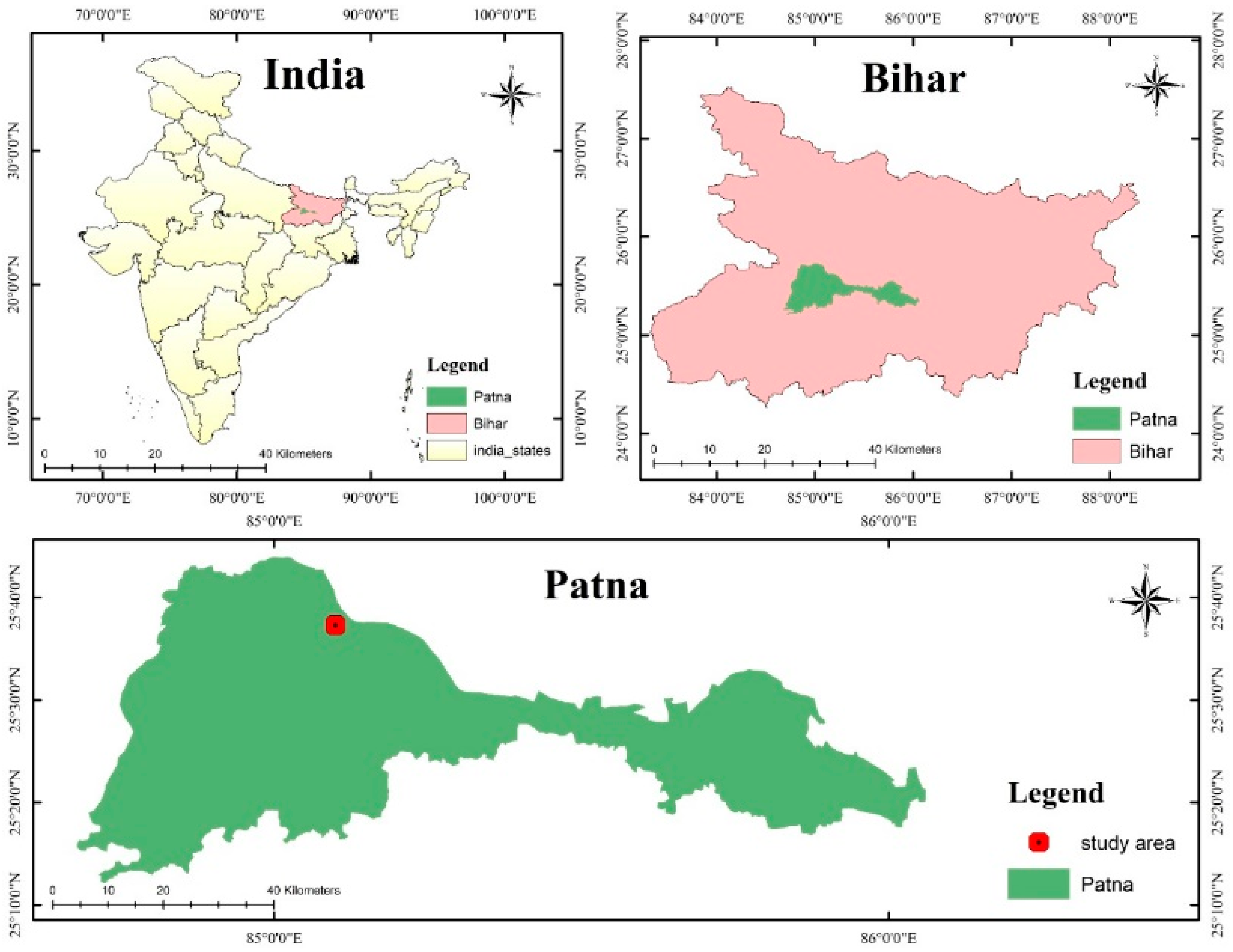
2.1. Study Area
2.2. Sampling Strategy
2.3. Chemical Characterization
2.4. Quality Assurance and Quality Control (QA/QC)
2.5. Statistical Analysis
2.6. Source Apportionment Study
2.7. Air Mass Back Trajectory
3. Results and Discussion
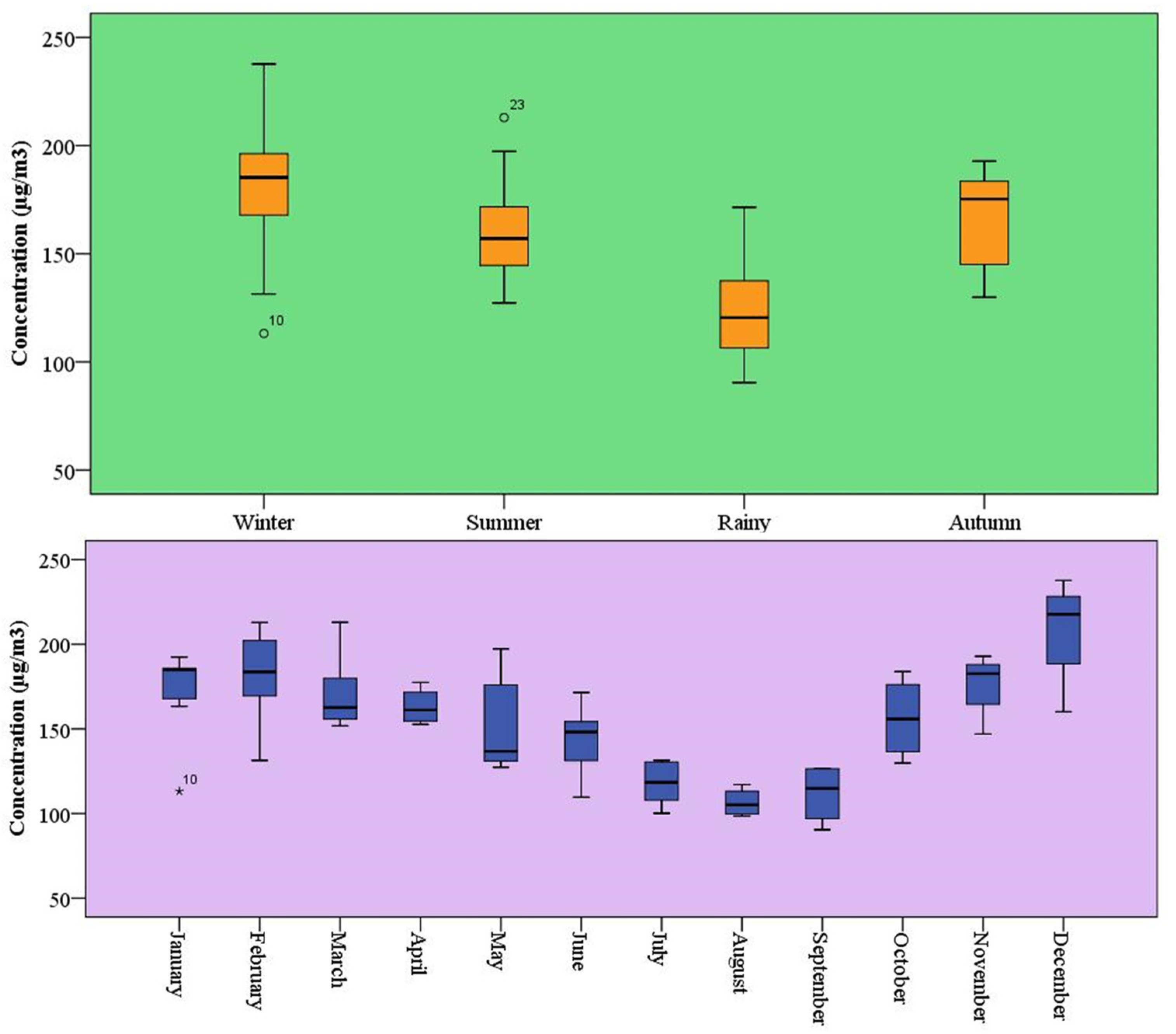
3.1. Concentration and Seasonal Variation of PM10
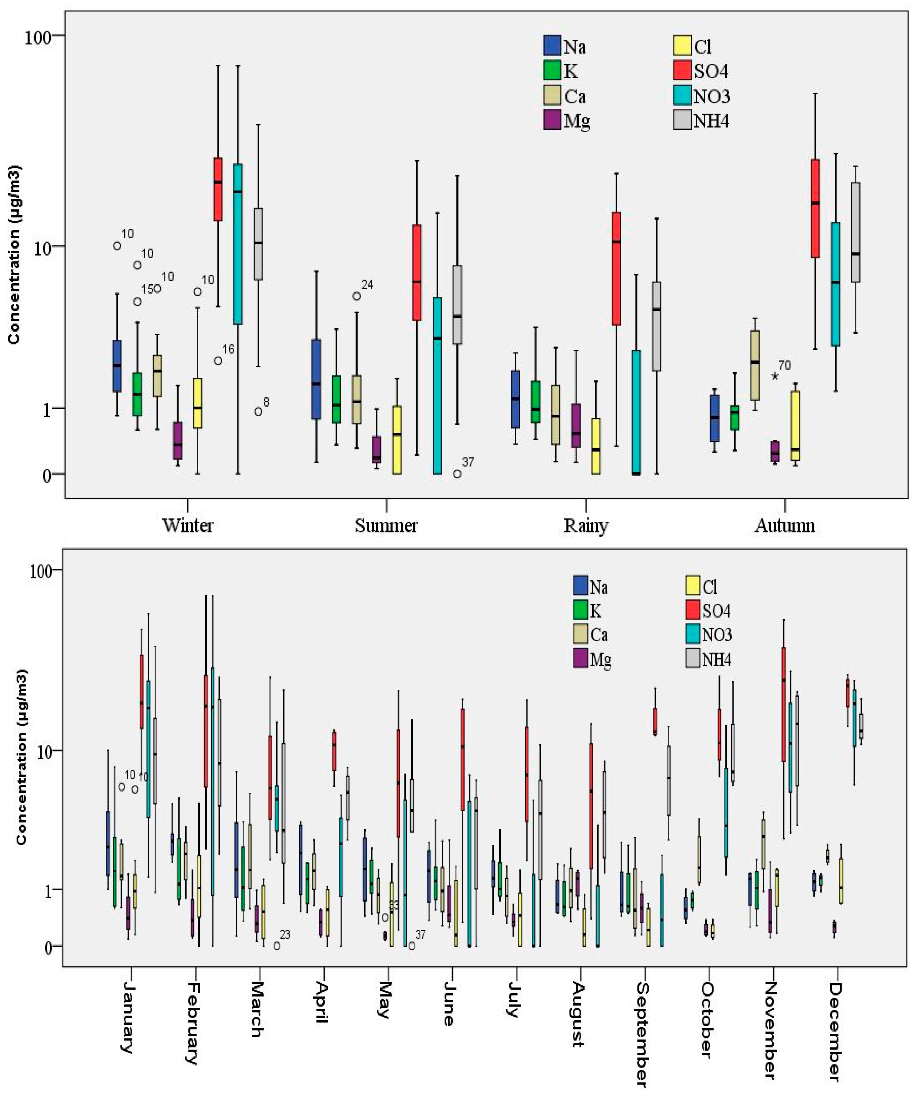
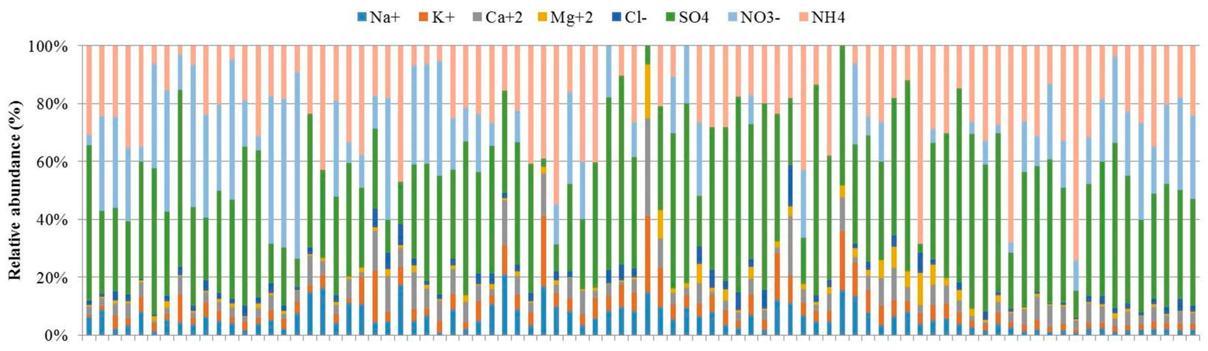
3.2. Concentration and Seasonal Variation of WSIIs
3.3. Relationship between PM and WSIIs
3.4. Source Apportionment Study
3.4.1. Molecular Diagnostic Ratio (MDR)
3.4.2. Principal Component Analysis (PCA)
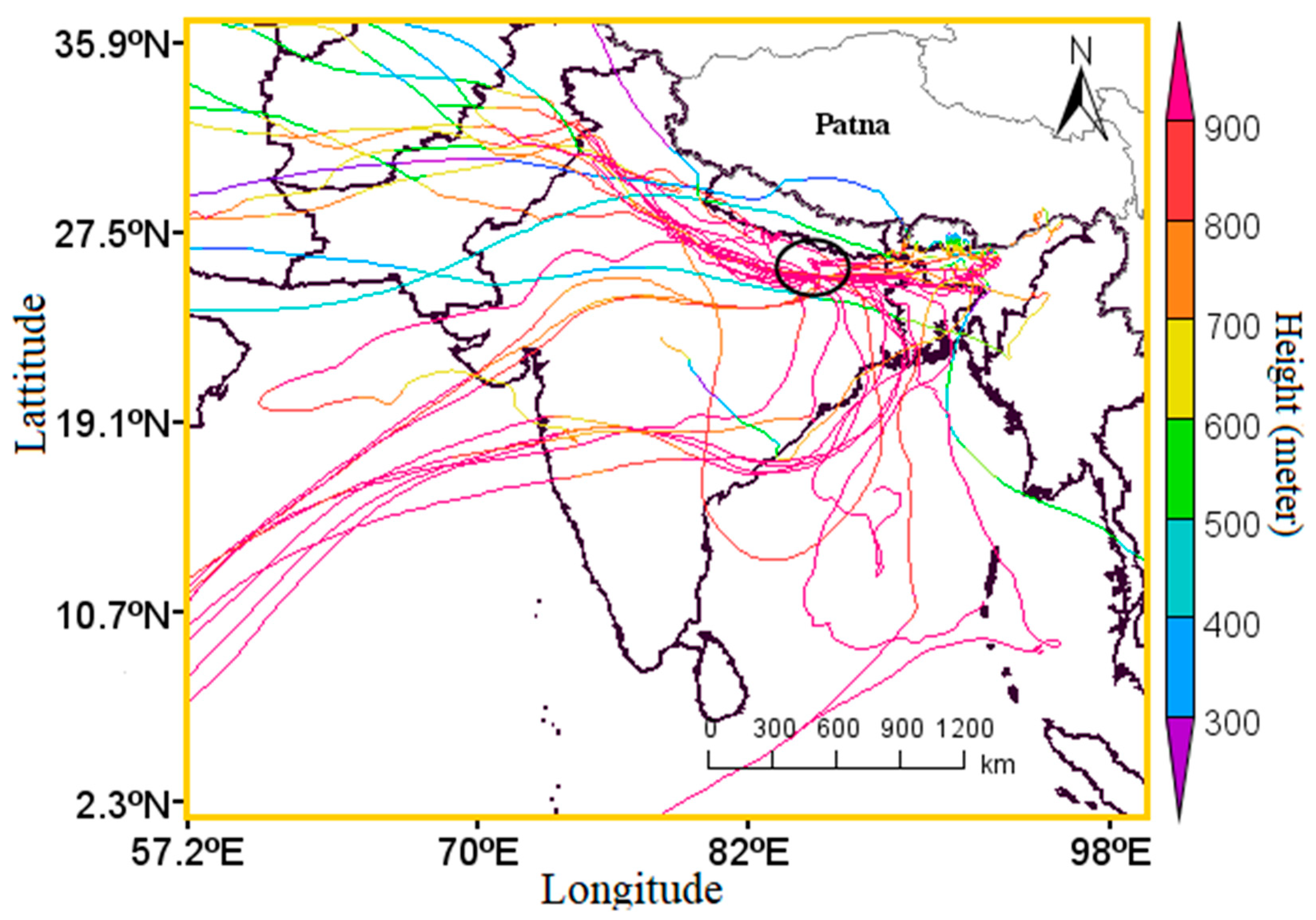
3.5. Backward Air Mass Trajectory
4. Conclusions
Author Contributions
Funding
Institutional Review Board Statement
Informed Consent Statement
Data Availability Statement
Conflicts of Interest
References
- Satheesh, S.K.; Ramanathan, V. Large differences in tropical aerosol forcing at the top of the atmosphere and Earth’s surface. Nature 2000, 405, 60–63. [Google Scholar] [CrossRef]
- Singh, J.; Gupta, P.; Gupta, D.; Verma, S.; Prakash, D.; Payra, S. Fine particulate pollution and ambient air quality: A case study over an urban site in Delhi, India. J. Earth Syst. Sci. 2020, 129, 226. [Google Scholar] [CrossRef]
- Wang, Y.; Wang, M.; Zhang, R.; Ghan, S.J.; Lin, Y.; Hu, J.; Pan, B.; Levy, M.; Jiang, J.H.; Molina, M.J. Assessing the effects of anthropogenic aerosols on Pacific storm track using a multiscale global climate model. Proc. Natl. Acad. Sci. USA 2014, 111, 6894–6899. [Google Scholar] [CrossRef]
- Sathe, Y.; Kulkarni, S.; Gupta, P.; Kaginalkar, A.; Islam, S.; Gargava, P. Application of Moderate Resolution Imaging Spectroradiometer (MODIS) Aerosol Optical Depth (AOD) and Weather Research Forecasting (WRF) model meteorological data for assessment of fine particulate matter (PM2.5) over India. Atmos. Pollut. Res. 2019, 10, 418–434. [Google Scholar] [CrossRef]
- Brauer, M.; Casadei, B.; Harrington, R.A.; Kovacs, R.; Sliwa, K.; WHF Air Pollution Expert Group. Taking a stand against air pollution—The impact on cardiovascular disease: A joint opinion from the world heart federation, American college of cardiology, American heart association, and the European society of cardiology. Circulation 2021, 143, 800–804. [Google Scholar] [CrossRef] [PubMed]
- WHO. Air Quality Guidelines: Global Update 2005: Particulate Matter, Ozone, Nitrogen Dioxide, and Sulfur Dioxide; World Health Organization: Geneva, Switzerland, 2006; Available online: http://www.euro.who.int/en/health-topics/environment-and-health/airquality/publications/pre2009/air-quality-guidelines.-global-update-2005.-particulatematter,-ozone,-nitrogen-dioxide-and-sulfur-dioxide (accessed on 24 February 2019).
- WHO. Ambient (Outdoor) Air Quality and Health; World Health Organization: Geneva, Switzerland, 2018; Available online: http://www.who.int/news-room/fact-sheets/detail/ambient-(outdoor)-air-quality-and-health (accessed on 14 September 2018).
- Dandona, L.; Dandona, R.; Kumar, G.A.; Shukla, D.K.; Paul, V.K.; Balakrishnan, K.; Prabhakaran, D.; Tandon, N.; Salvi, S.; Dash, A.P.; et al. Nations within a nation: Variations in epidemiological transition across the states of India, 1990–2016 in the Global Burden of Disease Study. Lancet 2017, 390, 2437–2460. [Google Scholar] [CrossRef] [PubMed]
- Balakrishnan, K.; Dey, S.; Gupta, T.; Dhaliwal, R.S.; Brauer, M.; Cohen, A.J.; Stanaway, J.D.; Beig, G.; Joshi, T.K.; Aggarwal, A.N.; et al. The impact of air pollution on deaths, disease burden, and life expectancy across the states of India: The Global Burden of Disease Study 2017. Lancet Planet. Health 2019, 3, e26–e39. [Google Scholar] [CrossRef] [PubMed]
- Munir, S.; Habeebullah, T.M.; Mohammed, A.M.; Morsy, E.A.; Rehan, M.; Ali, K. Analysing PM2.5 and its association with PM10 and meteorology in the arid climate of Makkah, Saudi Arabia. Aerosol Air Qual. Res. 2017, 17, 453–464. [Google Scholar] [CrossRef]
- Kong, S.; Han, B.; Bai, Z.; Chen, L.; Shi, J.; Xu, Z. Receptor modeling of PM2.5, PM10 and TSP in different seasons and long-range transport analysis at a coastal site of Tianjin, China. Sci. Total Environ. 2010, 408, 4681–4694. [Google Scholar] [CrossRef]
- Talbi, A.; Kerchich, Y.; Kerbachi, R.; Boughedaoui, M. Assessment of annual air pollution levels with PM1, PM2.5, PM10 and associated heavy metals in Algiers, Algeria. Environ. Pollut. 2018, 232, 252–263. [Google Scholar] [CrossRef]
- Dutta, A.; Jinsart, W. Risks to health from ambient particulate matter (PM2.5) to the residents of Guwahati city, India: An analysis of prediction model. Hum. Ecol. Risk Assess. Int. J. 2021, 27, 1094–1111. [Google Scholar] [CrossRef]
- Saxena, P.; Kumar, A.; Mahanta, S.K.; Sreekanth, B.; Patel, D.K.; Kumari, A.; Khan, A.H.; Kisku, G.C. Chemical characterization of PM10 and PM2.5 combusted firecracker particles during Diwali of Lucknow City, India: Air-quality deterioration and health implications. Environ. Sci. Pollut. Res. 2022, 29, 88269–88287. [Google Scholar] [CrossRef] [PubMed]
- Agarwal, S.; Aggarwal, S.G.; Okuzawa, K.; Kawamura, K. Size distributions of dicarboxylic acids, ketoacids, α-dicarbonyls, sugars, WSOC, OC, EC and inorganic ions in atmospheric particles over Northern Japan: Implication for long-range transport of Siberian biomass burning and East Asian polluted aerosols. Atmos. Chem. Phys. 2010, 10, 5839–5858. [Google Scholar] [CrossRef]
- Pavuluri, C.M.; Kawamura, K.; Aggarwal, S.G.; Swaminathan, T. Characteristics, seasonality and sources of carbonaceous and ionic components in the tropical aerosols from Indian region. Atmos. Chem. Phys. 2011, 11, 8215–8230. [Google Scholar] [CrossRef]
- Yttri, K.E.; Dye, C.; Kiss, G. Ambient aerosol concentrations of sugars and sugar-alcohols at four different sites in Norway. Atmos. Chem. Phys. 2007, 7, 4267–4279. [Google Scholar] [CrossRef]
- Maji, S.; Ahmed, S.; Siddiqui, W.A. Air quality assessment and its relation to potential health impacts in Delhi, India. Curr. Sci. 2015, 109, 902–909. [Google Scholar]
- Chowdhury, S.; Dey, S.; Smith, K.R. Ambient PM2.5 exposure and expected premature mortality to 2100 in India under climate change scenarios. Nat. Commun. 2018, 9, 318. [Google Scholar] [CrossRef] [PubMed]
- Kishore, N.; Srivastava, A.K.; Nandan, H.; Pandey, C.P.; Agrawal, S.; Singh, N.; Soni, V.K.; Bisht, D.S.; Tiwari, S.; Srivastava, M.K. Long-term (2005–2012) measurements of near-surface air pollutants at an urban location in the Indo-Gangetic Basin. J. Earth Syst. Sci. 2019, 128, 55. [Google Scholar] [CrossRef]
- Shyamsundar, P.; Springer, N.P.; Tallis, H.; Polasky, S.; Jat, M.L.; Sidhu, H.S.; Krishnapriya, P.P.; Skiba, N.; Ginn, W.; Ahuja, V.; et al. Fields on fire: Alternatives to crop residue burning in India. Science 2019, 365, 536–538. [Google Scholar] [CrossRef]
- Ojha, N.; Sharma, A.; Kumar, M.; Girach, I.; Ansari, T.U.; Sharma, S.K.; Singh, N.; Pozzer, A.; Gunthe, S.S. On the widespread enhancement in fne particulate matter across the Indo-Gangetic Plain towards winter. Sci. Rep. 2020, 10, 5862. [Google Scholar] [CrossRef]
- Srivastava, A.K.; Tripathi, S.N.; Dey, S.; Kanawade, V.P.; Tiwari, S. Inferring aerosol types over the Indo-Gangetic Basin from ground based sunphotometer measurements. Atmos. Res. 2012, 109–110, 64–75. [Google Scholar] [CrossRef]
- Srivastava, A.K.; Singh, S.; Tiwari, S.; Bisht, D.S. Contribution of anthropogenic aerosols in direct radiative forcing and atmospheric heating rate over Delhi in the Indo-Gangetic Basin. Environ. Sci. Pollut. Res. 2012, 19, 1144–1158. [Google Scholar] [CrossRef]
- Tiwari, S.; Srivastava, A.K.; Singh, A.K. Heterogeneity in pre-monsoon aerosol characteristics over the Indo-Gangetic Basin. Atmos. Environ. 2013, 77, 738–747. [Google Scholar] [CrossRef]
- Tiwari, S.; Srivastava, A.K.; Singh, A.K.; Singh, S. Identifcation of aerosol types over Indo-Gangetic Basin: Implications to optical properties and associated radiative forcing. Environ. Sci. Pollut. Res. 2015, 22, 12246–12260. [Google Scholar] [CrossRef]
- Kumar, M.; Parmar, K.S.; Kumar, D.B.; Mhawish, A.; Broday, D.M.; Mall, R.K.; Banerjee, T. Long-term aerosol climatology over Indo-Gangetic Plain: Trend, prediction and potential source felds. Atmos. Environ. 2018, 180, 37–50. [Google Scholar] [CrossRef]
- Bikkina, S.; Andersson, A.; Kirillova, E.N.; Holmstrand, H.; Tiwari, S.; Srivastava, A.K.; Bisht, D.S.; Gustafsson, Ö. Air quality in megacity Delhi affected by countryside biomass burning. Nat. Sustain. 2019, 2, 200–205. [Google Scholar] [CrossRef]
- Schwartz, J.; Dockery, D.W.; Neas, L.M. Is daily mortality associated specifically with fine particles? J. Air Waste Manag. Assoc. 1996, 46, 927–939. [Google Scholar] [CrossRef]
- Li, X.; Wang, S.; Duan, L.; Hao, J.; Nie, Y. Carbonaceous aerosol emissions from household biofuel combustion in China. Environ. Sci. Technol. 2009, 43, 6076–6081. [Google Scholar] [CrossRef]
- Ram, K.; Sarin, M.M.; Tripathi, S.N. Temporal trendsin atmospheric PM2.5, PM10, Elemental Carbon, Organic Carbon, Water soluble Organic Carbon and Optical Properties: Impact of biomass Burning Emissions in the Indo-Gangetic Plain. Environ. Sci. Technol. 2012, 46, 486–695. [Google Scholar] [CrossRef]
- Sharma, S.K.; Kumar, M.; Rohtash Gupta, N.C.; Saraswati Saxena, M.; Mandal, T.K. Characteristics of ambient ammonia over Delhi, India. Meteorol. Atmos. Phys. 2014, 124, 67–82. [Google Scholar] [CrossRef]
- Sharma, S.K.; Mandal, T.K.; Saxena, M.; Sharma, A.; Datta, A.; Saud, T. Variation of OC, EC, WSIC and trace metals of PM10 in Delhi, India. J. Atmos. Sol.-Terr. Phys. 2014, 113, 10–22. [Google Scholar] [CrossRef]
- Sen, A.; Ahammed, Y.N.; Arya, B.C.; Banerjee, T.; Reshma Begam, G.; Baruah, B.P.; Chatterjee, A.; Choudhuri, A.K.; Dhir, A.; Das, T.; et al. Atmospheric fine and coarse mode aerosols at different environments of India and the Bay of Bengal during winter-2014: Implications of a coordinated campaign. Mapan 2014, 29, 273–284. [Google Scholar] [CrossRef]
- Ram, K.; Sarin, M.M.; Tripathi, S.N. Inter-comparison of thermal and optical methods for determination of atmospheric black carbon and attenuation coefficient from an urban location in northern India. Atmos. Res. 2010, 97, 335–342. [Google Scholar] [CrossRef]
- Sharma, M.; Kishore, S.; Tripathi, S.N.; Behera, S.N. Role of atmospheric ammonia in the formation of inorganic secondary particulate matter: A study at Kanpur, India. J. Atmos. Chem. 2007, 58, 1–17. [Google Scholar] [CrossRef]
- Bond, T.C.; Doherty, S.J.; Fahey, D.W.; Forster, P.M.; Berntsen, T.; DeAngelo, B.J.; Flanner, M.G.; Ghan, S.; Kärcher, B.; Koch, D.; et al. Bounding the role of black carbon in the climate system: A scientific assessment. J. Geophys. Res. Atmos. 2013, 118, 5380–5552. [Google Scholar] [CrossRef]
- Kumar, A.; Yadav, I.C.; Shukla, A.; Devi, N.L. Seasonal variation of PM2.5 in the central Indo-Gangetic Plain (Patna) of India: Chemical characterization and source assessment. SN Appl. Sci. 2020, 2, 1366. [Google Scholar] [CrossRef]
- Devi, N.L.; Kumar, A.; Yadav, I.C.; Szidat, S.; Sharma, R. Source Apportionment of Fine Particulate Matter in Middle Indo-Gangetic Plain by Coupled Radiocarbon–Molecular Organic Tracer Method. Atmos. Pollut. Res. 2024, 15, 102231. [Google Scholar] [CrossRef]
- Devi, N.L.; Kumar, A.; Yadav, I.C. PM10 and PM2.5 in Indo-Gangetic Plain (IGP) of India: Chemical characterization, source analysis, and transport pathways. Urban Clim. 2020, 33, 100663. [Google Scholar] [CrossRef]
- Banerjee, T.; Murari, V.; Kumar, M.; Raju, M.P. Source apportionment of airborne particulates through receptor modeling: Indian scenario. Atmos. Res. 2015, 164, 167–187. [Google Scholar] [CrossRef]
- Ghosh, S.; Rabha, R.; Chowdhury, M.; Padhy, P.K. Source and chemical species characterization of PM10 and human health risk assessment of semi-urban, urban and industrial areas of West Bengal, India. Chemosphere 2018, 207, 626–636. [Google Scholar] [CrossRef]
- Filonchyk, M.; Peterson, M.; Hurynovich, V. Air pollution in the Gobi Desert region: Analysis of duststorm events. Q. J. R. Meteorol. Soc. 2021, 147, 1097–1111. [Google Scholar] [CrossRef]
- Tiwari, S.; Dumka, U.C.; Kaskaoutis, D.G.; Ram, K.; Panicker, A.S.; Srivastava, M.K.; Pandey, A.K. Aerosol chemical characterization and role of carbonaceous aerosol on radiative effect over Varanasi in central Indo-Gangetic Plain. Atmos. Environ. 2016, 125, 437–449. [Google Scholar] [CrossRef]
- Bikkina, S.; Andersson, A.; Ram, K.; Sarin, M.M.; Sheesley, R.J.; Kirillova, E.N.; Gustafsson, Ö. Carbon isotope-constrained seasonality of carbonaceous aerosol sources from an urban location (Kanpur) in the Indo-Gangetic Plain. J. Geophys. Res. Atmos. 2017, 122, 4903–4923. [Google Scholar] [CrossRef]
- Shahid, I.; Kistler, M.; Mukhtar, A.; Ghauri, B.M.; Ramirez-Santa Cruz, C.; Bauer, H.; Puxbaum, H. Chemical characterization and mass closure of PM10 and PM2.5 at an urban site in Karachi–Pakistan. Atmos. Environ. 2016, 128, 114–123. [Google Scholar] [CrossRef]
- Alam, K.; Rahman, N.; Khan, H.U.; Haq, B.S.; Rahman, S. Particulate matter and its source apportionment in Peshawar, Northern Pakistan. Aerosol Air Qual. Res. 2015, 15, 634–647. [Google Scholar] [CrossRef]
- Rengarajan, R.; Sudheer, A.K.; Sarin, M.M. Wintertime PM2.5 and PM10 carbonaceous and inorganic constituents from urban site in western India. Atmos. Res. 2011, 102, 420–431. [Google Scholar] [CrossRef]
- Venkataraman, C.; Thomas, S.; Kulkarni, P. Size distributions of polycyclic aromatic hydrocarbons—Gas/particle partitioning to urban aerosols. J. Aerosol Sci. 1999, 30, 759–770. [Google Scholar] [CrossRef]
- Sharma, S.K.; Mandal, T.K.; Saxena, M.; Sharma, A.; Gautam, R. Source apportionment of PM10 by using positive matrix factorization at an urban site of Delhi, India. Urban Clim. 2014, 10, 656–670. [Google Scholar] [CrossRef]
- Bulbul, G.; Shahid, I.; Chishtie, F.; Shahid, M.Z.; Hundal, R.A.; Zahra, F.; Shahzad, M.I. PM10 Sampling and AOD Trends during 2016 Winter Fog Season in the Islamabad Region. Aerosol Air Qual. Res. 2018, 18, 188–199. [Google Scholar] [CrossRef]
- Bhuyan, P.; Deka, P.; Prakash, A.; Balachandran, S.; Hoque, R.R. Chemical characterization and source apportionment of aerosol over mid Brahmaputra Valley, India. Environ. Pollut. 2018, 234, 997–1010. [Google Scholar] [CrossRef]
- Chithra, V.S.; Nagendra, S.S. Chemical and morphological characteristics of indoor and outdoor particulate matter in an urban environment. Atmos. Environ. 2013, 77, 579–587. [Google Scholar] [CrossRef]
- Sharma Sharma, S.K.; Mandal, T.K.; Jain, S.; Saraswati Sharma, A.; Saxena, M. Source apportionment of PM2.5 in Delhi, India using PMF model. Bull. Environ. Contam. Toxicol. 2016, 97, 286–293. [Google Scholar] [CrossRef] [PubMed]
- Ram, K.; Sarin, M.M. Atmospheric 210Pb, 210Po and 210Po/210Pb activity ratio in urban aerosols: Temporal variability and impact of biomass burning emission. Tellus B: Chem. Phys. Meteorol. 2012, 64, 17513. [Google Scholar] [CrossRef]
- Panda, S.; Nagendra, S.S. Chemical and morphological characterization of respirable suspended particulate matter (PM10) and associated heath risk at a critically polluted industrial cluster. Atmos. Pollut. Res. 2018, 9, 791–803. [Google Scholar] [CrossRef]
- Arif, M.; Kumar, R.; Kumar, R.; Eric, Z.; Gourav, P. Ambient black carbon, PM2.5 and PM10 at Patna: Influence of anthropogenic emissions and brick kilns. Sci. Total Environ. 2018, 624, 1387–1400. [Google Scholar] [CrossRef] [PubMed]
- Yu, L.; Wang, G.; Zhang, R.; Zhang, L.; Song, Y.; Wu, B.; Li, X.; An, K.; Chu, J. Characterization and source apportionment of PM2.5 in an urban environment in Beijing. Aerosol Air Qual. Res. 2013, 13, 574–583. [Google Scholar] [CrossRef]
- Yao, L.; Yang, L.; Yuan, Q.; Yan, C.; Dong, C.; Meng, C.; Sui, X.; Yang, F.; Lu, Y.; Wang, W. Sources apportionment of PM2.5 in a background site in the North China Plain. Sci. Total Environ. 2016, 541, 590–598. [Google Scholar] [CrossRef] [PubMed]
- Khillare, P.S.; Sarkar, S. Airborne inhalable metals in residential areas of Delhi, India: Distribution, source apportionment and health risks. Atmos. Pollut. Res. 2012, 3, 46–54. [Google Scholar] [CrossRef]
- Ho, K.F.; Lee, S.C.; Chan, C.K.; Jimmy, C.Y.; Chow, J.C.; Yao, X.H. Characterization of chemical species in PM2.5 and PM10 aerosols in Hong Kong. Atmos. Environ. 2003, 37, 31–39. [Google Scholar] [CrossRef]
- Wang, X.; Bi, X.; Sheng, G.; Fu, J. Chemical composition and sources of PM10 and PM2.5 aerosols in Guangzhou, China. Environ. Monit. Assess. 2006, 119, 425–439. [Google Scholar] [CrossRef]
- Ghosh, S.; Gupta, T.; Rastogi, N.; Gaur, A.; Misra, A.; Tripathi, S.N.; Dwivedi, A.K.; Paul, D.; Tare, V.; Prakash, O.; et al. Chemical characterization of summertime dust events at Kanpur: Insight into the sources and level of mixing with anthropogenic emissions. Aerosol Air Qual. Res. 2014, 14, 879–891. [Google Scholar] [CrossRef]
- Draxler, R.R.; Hess, G.D. An overview of the HYSPLIT_4 modelling system for trajectories. Aust. Meteorol. Mag. 1998, 47, 295–308. [Google Scholar]
- Cheng, Z.; Wang, S.; Jiang, J.; Fu, Q.; Chen, C.; Xu, B.; Yu, J.; Fu, X.; Hao, J. Long-term trend of haze pollution and impact of particulate matter in the Yangtze River Delta, China. Environ. Pollut. 2013, 182, 101–110. [Google Scholar] [CrossRef] [PubMed]
- Arimoto, R.; Duce, R.A.; Savoie, D.L.; Prospero, J.M.; Talbot, R.; Cullen, J.D.; Tomza, U.; Lewis, N.F.; Ray, B.J. Relationships among aerosol constituents from Asia and the North Pacific during PEM-West A. J. Geophys. Res. Atmos. 1996, 101, 2011–2023. [Google Scholar] [CrossRef]
- Rushdi, A.I.; Al-Mutlaq, K.F.; Al-Otaibi, M.; El-Mubarak, A.H.; Simoneit, B.R. Air quality and elemental enrichment factors of aerosol particulate matter in Riyadh City, Saudi Arabia. Arab. J. Geosci. 2013, 6, 585–599. [Google Scholar] [CrossRef]
- Shahsavani, A.; Naddafi, K.; Haghighifard, N.J.; Mesdaghinia, A.; Yunesian, M.; Nabizadeh, R.; Arahami, M.; Sowlat, M.H.; Yarahmadi, M.; Saki, H.; et al. The evaluation of PM10, PM2.5, and PM1 concentrations during the Middle Eastern Dust (MED) events in Ahvaz, Iran, from april through september 2010. J. Arid. Environ. 2012, 77, 72–83. [Google Scholar] [CrossRef]
- Shukla, S.P.; Sharma, M. Source apportionment of atmospheric PM10 in Kanpur, India. Environ. Eng. Sci. 2008, 25, 849–862. [Google Scholar] [CrossRef]
- Liu, B.; Wu, J.; Zhang, J.; Wang, L.; Yang, J.; Liang, D.; Dai, Q.; Bi, X.; Feng, Y.; Zhang, Y.; et al. Characterization and source apportionment of PM2.5 based on error estimation from EPA PMF 5.0 model at a medium city in China. Environ. Pollut. 2017, 222, 10–22. [Google Scholar] [CrossRef]
- Ilizarbe-Gonzáles, G.M.; Rojas-Quincho, J.P.; Cabello-Torres, R.J.; Ugarte-Alvan, C.A.; Reynoso-Quispe, P.; Valdiviezo-Gonzales, L.G. Chemical characteristics and identification of PM10 sources in two districts of Lima, Peru. Dyna 2020, 87, 57–65. [Google Scholar] [CrossRef]
- Chu, D.A.; Kaufman, Y.J.; Zibordi, G.; Chern, J.D.; Mao, J.; Li, C.; Holben, B.N. Global monitoring of air pollution over land from the Earth Observing System-Terra Moderate Resolution Imaging Spectroradiometer (MODIS). J. Geophys. Res. Atmos. 2003, 108, ACH4.1–ACH4.18. [Google Scholar] [CrossRef]

| Sampling Location | Sampling Periods | Winter | Summer | Rainy | Autumn | References |
|---|---|---|---|---|---|---|
| Patna | January 2018–December 2018 | 185 | 157 | 121 | 175 | This study |
| Ahmedabad | December 2006–January 2007 | 171 | - | - | - | [48] |
| Brahmaputra Velley | December 2010–October 2014 | 96.1 | 52.6 | 22.1 | 45.3 | [52] |
| Chennai | Octoer 2011–May 2012 | 170 | 150 | 158 | - | [53] |
| Delhi | January 2010–December 2011 | 241 | 193 | 140 | - | [54] |
| Hissar | December 2004 | 169 | - | - | - | [31] |
| Prayagraj | 254 | - | - | - | ||
| Kanpur | October 2008 | - | - | - | 243 | [55] |
| Manali, India | November 2014–May 2016 | 131 | 107 | 103 | 115 | [56] |
| Patna | January–December 2015 | 109 | 98.3 | 63 | 64.1 | [57] |
| Varanasi | April–July 2011 | - | 210 | 131 | - | [44] |
| Delhi | December 2008–November 2009 | 182 | 211 | 140 | - | [58] |
| Islamabad | January–February 2016 | 177 | - | - | - | [51] |
| Hong Kong | November2000–February 2001 | 78.9 | - | - | - | [59] |
| Guangzhou | August–September 2004 | - | - | 138 | - | [60] |
| Locations | Sampling Year | Season | K+ | Na+ | Ca+2 | Mg+2 | SO4−2 | NO3− | NH4+ | Cl− | References |
|---|---|---|---|---|---|---|---|---|---|---|---|
| Patna | January–December 2018 | Winter | 1.31 | 2.13 | 1.95 | 0.36 | 20.58 | 18.51 | 10.39 | 1.01 | This study |
| Summer | 1.07 | 1.60 | 1.14 | 0.19 | 6.55 | 3.20 | 4.30 | 0.52 | |||
| Rainy | 0.97 | 1.21 | 0.84 | 0.53 | 10.55 | 1.38 | 4.65 | 0.29 | |||
| Autumn | 0.91 | 0.82 | 2.25 | 0.24 | 17.39 | 7.02 | 9.21 | 0.30 | |||
| Kanpur | April–July 2011 | Summer | - | - | - | - | 6.54 | 4.97 | 4.11 | 2.68 | [61] |
| Brahmaputra Valley | December–October 2014 | Winter | 2.1 | 2.14 | 0.66 | 0.09 | 5.02 | 2.14 | 2.20 | 1.10 | [52] |
| Summer | 1.27 | 1.97 | 0.86 | 0.13 | 3.05 | 1.10 | 1.02 | 1.21 | |||
| Rainy | 0.66 | 1.47 | 0.38 | 0.05 | 1.15 | 0.49 | 0.43 | 0.84 | |||
| Autumn | 0.96 | 1.59 | 0.57 | 0.08 | 1.68 | 0.65 | 0.61 | 1.12 | |||
| Ahemadabad | December–January 2007 | Winter | 1.4 | 0.94 | 6.1 | 0.3 | 13.8 | 7.2 | 3.7 | 0.5 | [48] |
| Hisar | December 2004 | Winter | 2.6 | 0.73 | 3.5 | 0.36 | 12.33 | 14.56 | 6.6 | 0.4 | [31] |
| Allahabad | 2.4 | 0.66 | 5.7 | 0.6 | 17.66 | 9.26 | 6.23 | 0.16 | |||
| Manali | November 2014–May 2016 | Winter | 2.70 | 5.66 | 3.29 | 1.79 | 6.07 | 5.09 | 4.5 | 4.41 | [56] |
| Summer | 2.51 | 3.56 | 3.07 | 1.26 | 5.94 | 3.24 | 3.51 | 3.44 | |||
| Rainy | 2.39 | 2.83 | 2.23 | 1.02 | 4.34 | 4.16 | 3.71 | 3.32 | |||
| Autumn | 2.93 | 4.38 | 2.32 | 1.27 | 5.56 | 5.27 | 4.24 | 3.53 | |||
| Delhi | January 2010–December 2011 | Winter | 1.7 | 2.3 | 4.8 | 0.7 | 11.6 | 14.1 | 9.6 | 5.0 | [54] |
| Summer | 1.5 | 3.3 | 4.7 | 0.6 | 9.2 | 5.1 | 2.6 | 3.5 | |||
| Autumn | 1.7 | 4.2 | 5.2 | 0.6 | 8.8 | 4.9 | 2.5 | 2.5 | |||
| Chennai, India | October–November 2011 April–May 2012 | Winter | 1.70 | 3.85 | 3.90 | 0.19 | 10.57 | 5.92 | 6.54 | 3.59 | [53] |
| Summer | 2.07 | 5.98 | 4.99 | 0.25 | 12.13 | 4.23 | 2.78 | 3.65 | |||
| Rainy | 0.87 | 3.22 | 3.35 | 0.33 | 9.96 | 5.90 | 7.53 | 3.18 | |||
| Varanasi, India | April–July 2011 | Summer | 2.35 | 2.2 | 3.6 | 0.55 | 5.3 | 4.5 | 1.21 | 1.8 | [26] |
| Rainy | 1.15 | 2.7 | 2.8 | 0.45 | 4.3 | 2.6 | 0.7 | 2.4 |
| PM10 | Na | K | Ca | Mg | Cl | SO4 | NO3 | |
|---|---|---|---|---|---|---|---|---|
| Na | 0.11 | |||||||
| K | 0.05 | 0.538 ** | ||||||
| Ca | 0.31 ** | 0.486 ** | 0.412 ** | |||||
| Mg | −0.14 | 0.12 | 0.332 ** | 0.21 | ||||
| Cl | 0.22 | 0.422 ** | 0.599 ** | 0.414 ** | 0.03 | |||
| SO4 | 0.35 ** | 0.335 ** | 0.378 ** | 0.378 ** | 0.19 | 0.597 ** | ||
| NO3 | 0.299 ** | 0.382 ** | 0.584 ** | 0.417 ** | 0.279 * | 0.599 ** | 0.494 ** | |
| NH4 | 0.10 | 0.523 ** | 0.416 ** | 0.428 ** | 0.06 | 0.536 ** | 0.467 ** | 0.458 ** |
| Months | Cl−/Mg2+ | SO42−/Mg2+ | Na+/Mg2+ | K+/Mg2+ | Ca2+/Mg2+ | Cl−/Na+ | K+/Na+ | Mg2+/Na+ | Ca2+/Na+ | SO42−/Na+ | SO4−2/K+ | NO3−/SO4−2 | Cl−/K+ | Na+/Ca2+ | K+/Ca2+ | Mg2+/Ca2+ | Cl−/Ca2+ | NO3−/Ca2+ | SO42−/Ca2+ |
|---|---|---|---|---|---|---|---|---|---|---|---|---|---|---|---|---|---|---|---|
| January | 2.53 | 41.3 | 5.91 | 3.95 | 3.67 | 0.43 | 0.67 | 0.17 | 0.62 | 6.98 | 10.4 | 0.85 | 0.64 | 1.61 | 1.07 | 0.27 | 0.69 | 9.56 | 11.2 |
| February | 2.83 | 42.3 | 5.23 | 3.69 | 3.85 | 0.54 | 0.71 | 0.19 | 0.74 | 8.08 | 11.4 | 0.96 | 0.77 | 1.36 | 0.96 | 0.26 | 0.74 | 10.5 | 10.9 |
| March | 1.46 | 21.3 | 5.98 | 3.71 | 5.61 | 0.24 | 0.62 | 0.17 | 0.94 | 3.58 | 5.77 | 0.59 | 0.39 | 1.07 | 0.66 | 0.18 | 0.26 | 2.24 | 3.81 |
| April | 1.63 | 29.1 | 6.17 | 3.51 | 4.54 | 0.26 | 0.57 | 0.16 | 0.74 | 4.73 | 8.30 | 0.25 | 0.46 | 1.36 | 0.77 | 0.22 | 0.36 | 1.63 | 6.42 |
| May | 4.00 | 51.8 | 10.7 | 8.31 | 5.69 | 0.37 | 0.77 | 0.09 | 0.53 | 4.82 | 6.23 | 0.30 | 0.48 | 1.89 | 1.46 | 0.18 | 0.70 | 2.74 | 9.11 |
| June | 0.65 | 12.1 | 1.77 | 1.71 | 1.37 | 0.37 | 0.97 | 0.56 | 0.77 | 6.83 | 7.07 | 0.21 | 0.38 | 1.30 | 1.25 | 0.73 | 0.48 | 1.83 | 8.85 |
| July | 1.46 | 21.4 | 3.84 | 3.78 | 2.43 | 0.38 | 0.99 | 0.26 | 0.63 | 5.58 | 5.66 | 0.15 | 0.39 | 1.58 | 1.56 | 0.41 | 0.60 | 1.36 | 8.81 |
| August | 0.26 | 5.71 | 0.77 | 0.73 | 0.98 | 0.33 | 0.94 | 1.30 | 1.28 | 7.42 | 7.86 | 0.13 | 0.35 | 0.78 | 0.74 | 1.02 | 0.26 | 0.74 | 5.81 |
| September | 0.45 | 23.6 | 1.69 | 1.64 | 1.58 | 0.27 | 0.97 | 0.59 | 0.94 | 14.0 | 14.4 | 0.05 | 0.28 | 1.07 | 1.04 | 0.63 | 0.29 | 0.72 | 14.9 |
| October | 0.95 | 62.8 | 2.77 | 3.45 | 9.27 | 0.34 | 1.25 | 0.36 | 3.34 | 22.6 | 18.1 | 0.40 | 0.28 | 0.30 | 0.37 | 0.11 | 0.10 | 2.72 | 6.77 |
| November | 1.74 | 41.0 | 1.65 | 1.63 | 4.15 | 1.06 | 0.99 | 0.61 | 2.52 | 24.9 | 25.1 | 0.50 | 1.07 | 0.40 | 0.39 | 0.24 | 0.42 | 4.93 | 9.87 |
| December | 5.12 | 83.8 | 4.58 | 4.77 | 7.81 | 1.12 | 1.04 | 0.22 | 1.71 | 18.3 | 17.5 | 0.78 | 1.07 | 0.59 | 0.61 | 0.13 | 0.66 | 8.40 | 10.7 |
| WSIIs | Winter | Summer | Rainy | Autumn | ||||||
|---|---|---|---|---|---|---|---|---|---|---|
| PC1 | PC2 | PC1 | PC2 | PC3 | PC1 | PC2 | PC3 | PC1 | PC3 | |
| Na+ | 0.845 | 0.002 | 0.872 | 0.179 | 0.251 | 0.367 | 0.747 | 0.337 | 0.942 | −0.141 |
| K+ | 0.728 | 0.534 | 0.267 | −0.099 | 0.663 | 0.663 | 0.528 | 0.185 | 0.795 | 0.533 |
| Ca2+ | 0.897 | 0.038 | 0.206 | 0.838 | 0.018 | 0.829 | 0.052 | 0.141 | 0.527 | 0.186 |
| Mg2+ | 0.009 | 0.920 | 0.453 | 0.710 | −0.006 | 0.894 | −0.004 | −0.090 | 0.317 | 0.815 |
| Cl− | 0.869 | 0.358 | −0.215 | 0.103 | 0.857 | −0.406 | −0.623 | 0.261 | 0.817 | 0.131 |
| SO42− | 0.515 | 0.305 | 0.525 | 0.358 | 0.426 | −0.136 | 0.221 | 0.849 | 0.677 | 0.715 |
| NO3− | 0.348 | 0.842 | −0.171 | 0.907 | 0.039 | −0.194 | 0.700 | −0.037 | 0.762 | 0.475 |
| NH4+ | 0.839 | 0.307 | 0.903 | −0.004 | −0.191 | 0.320 | −0.282 | 0.685 | 0.072 | −0.888 |
| Eigenvalue | 4.717 | 1.336 | 2.950 | 1.597 | 1.364 | 2.902 | 1.414 | 1.349 | 4.705 | 1.452 |
| Variance (%) | 58.96 | 16.69 | 36.87 | 19.96 | 17.05 | 36.27 | 17.67 | 16.86 | 58.81 | 18.15 |
Disclaimer/Publisher’s Note: The statements, opinions and data contained in all publications are solely those of the individual author(s) and contributor(s) and not of MDPI and/or the editor(s). MDPI and/or the editor(s) disclaim responsibility for any injury to people or property resulting from any ideas, methods, instructions or products referred to in the content. |
© 2024 by the authors. Licensee MDPI, Basel, Switzerland. This article is an open access article distributed under the terms and conditions of the Creative Commons Attribution (CC BY) license (https://creativecommons.org/licenses/by/4.0/).
Share and Cite
Devi, N.L.; Chandra Yadav, I.; Kumar, A. Estimation of Particulate Matter (PM10) Over Middle Indo-Gangetic Plain (Patna) of India: Seasonal Variation and Source Apportionment. Atmosphere 2024, 15, 878. https://doi.org/10.3390/atmos15080878
Devi NL, Chandra Yadav I, Kumar A. Estimation of Particulate Matter (PM10) Over Middle Indo-Gangetic Plain (Patna) of India: Seasonal Variation and Source Apportionment. Atmosphere. 2024; 15(8):878. https://doi.org/10.3390/atmos15080878
Chicago/Turabian StyleDevi, Ningombam Linthoingambi, Ishwar Chandra Yadav, and Amrendra Kumar. 2024. "Estimation of Particulate Matter (PM10) Over Middle Indo-Gangetic Plain (Patna) of India: Seasonal Variation and Source Apportionment" Atmosphere 15, no. 8: 878. https://doi.org/10.3390/atmos15080878