Using the Multiple-Sensor-Based Frost Observation System (MFOS) for Image Object Analysis and Model Prediction Evaluation in an Orchard

Abstract

Accurate frost observations are crucial for developing and validating frost prediction models. In 2022, the multi-sensor-based automatic frost observation system (MFOS), including an RGB camera, a thermal infrared camera, a leaf wetness sensor (LWS), LED lighting, and three glass plates, was developed to replace the naked-eye observation of frost. The MFOS, herein installed and operated in an apple orchard, provides temporally high-resolution frost observations that show the onset, end, duration, persistence, and discontinuity of frost more clearly than conventional naked-eye observations. This study introduces recent additions to the MFOS and presents the results of its application to frost weather analysis and forecast evaluation in an orchard in South Korea. The NCAM’s Weather Research and Forecasting (WRF) model was employed as a weather forecast model. The main findings of this study are as follows: (1) The newly added image-based object detection capabilities of the MFOS helped with the extraction and quantitative comparison of surface temperature data for apples, leaves, and the LWS. (2) The resolution matching of the RGB and thermal infrared images was made successful by resizing the images, matching them according to horizontal movement, and conducting apple-centered averaging. (3) When applied to evaluate the frost-point predictions of the numerical weather model at one-hour intervals, the results showed that the MFOS could be used as a much more objective tool to verify the accuracy and characteristics of frost predictions compared to the naked-eye view. (4) Higher-resolution and realistic land-cover and vegetation representation are necessary to improve frost forecasts using numerical grid models based on land–atmosphere physics.

1. Introduction

The American Meteorological Society (https://www.ametsoc.org/index.cfm/ams/publications/glossary-of-meteorology (accessed on 15 May 2024)) defines frost as the direct sublimation of water vapor into ice, forming a fuzzy layer of ice crystals on cold objects. Crops are no exception to this. The onset, end, and intensity of frost depend on the behavior of the temperature, humidity, wind, and precipitation at or near the ground surface and are influenced by the duration of pre-dawn low temperatures [1]. Frost also depends on the characteristics of the surrounding terrain where the crops are located, the crop type, and the crop’s physiological stage, and can vary from a general freeze, to hoarfrost (or white frost), to a dry freeze (or black frost). Spring frost causes tissue damage and the destruction of plant reproductive organs and flower surfaces, leading to catastrophic losses for farmers [2]. In South Korea, 7211 ha of crops, such as apple fruits and chili peppers, are reported to have been damaged by frost in inland and mountainous areas [3].

Frost observations form the basis of frost forecasting. The Korea Meteorological Administration conducts frost observations with the naked eye at 23 human-crewed stations in the synoptic meteorological observation network in the morning and afternoon [4]. Although naked-eye frost observation is a crucial activity, (1) objective and quantitative measurements are not possible owing to human subjectivity, (2) the temporal observation frequency is very low (twice a day), and (3) the observation site is not a farm orchard or farmland that is damaged by frost, but a grassy field. Thus, there are difficulties in analyzing and predicting frost that occurs on farms.

Researchers have examined frost observations in various ways in recent years, not just at ground level. Groh et al. [5] studied the development of dew and frost in low mountains and alpine meadows using the mass changes in a lysimeter, air temperature, relative humidity, and surface temperature. Goswami et al. [6] used Parrot Sequoia multispectral cameras (green [550 nm], red [690 nm], Red Edge [735 nm], and NIR [790 nm]) for UAV remote sensing from crewless aerial vehicles to assess crop health, stress levels, and nutritional status. Tait and Zheng [7] created a frost occurrence map using satellite data, and Wang et al. [8] observed frost using MODIS satellite images by constructing a spring frost damage index. Valjarević et al. [9] proposed a grid-based model that interpolates dew-point temperature data from satellite and meteorological station data. However, there is a lack of research evaluating grid-based frost prediction models and orchard field-based image observation systems.

Frost image analysis using high-resolution imagery has mainly been limited to image classification or damage indexing using vegetation indices based on satellite imagery. This is because small-scale weather events such as frost are challenging to observe using satellite imagery. The study of automatic frost observation in agricultural fields in Korea began with a method using RGB cameras [10], and the authors of [11] presented a method using RGB, thermal infrared cameras, and leaf wetness sensors (LWSs). Subsequently, the authors of [12] solved the problem in which RGB cameras cannot be used at night by installing triplet glass plates, blackening the surface of the LWS, and installing LED lights at night, and introduced a method for extracting surface temperature values from image data to solve the problem in which thermal infrared cameras cannot observe the actual temperature. This study aims to demonstrate the results of complementing the multiple-sensor-based frost observation system (MFOS) with image post-processing, extracting the surface temperature of fruit tree elements, and using it to validate temporally high-resolution frost forecasts.

2. Materials and Methods

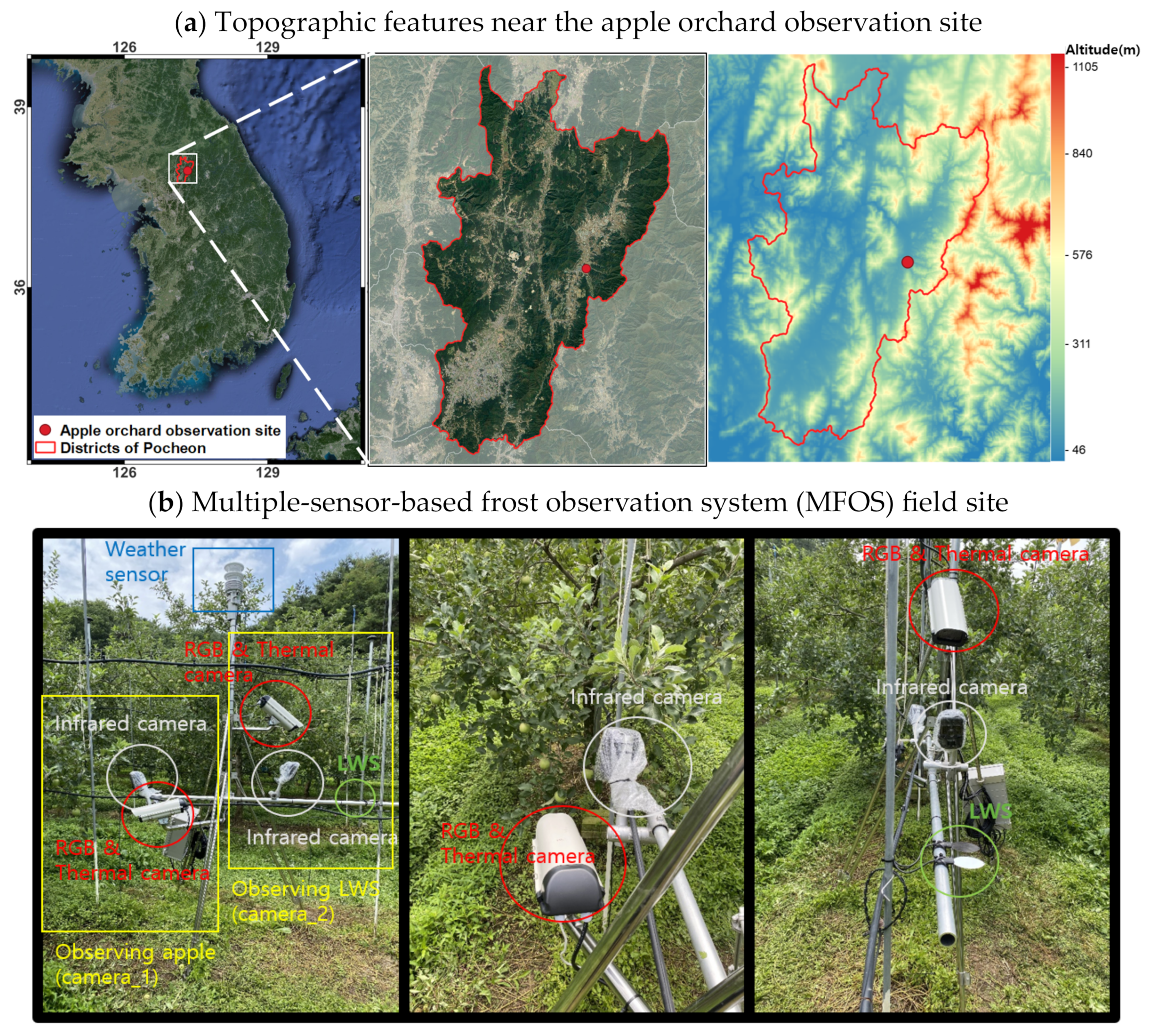
2.1. Study Area (Apple Farm)

The study site was an open-field apple orchard in Hwadae-ri, Ildong-myeon, Pocheon-si, Gyeonggi-do, South Korea, that does not use plastic wrapping during fruit growth (Figure 1). The orchard is located in a basin surrounded by mountainous land at an altitude of 800 m above sea level to the east and 500 m to the west. With the cooperation of the orchard owner, the observation system was positioned at a distance adjacent to the apple trees and set up so that the imaging equipment could capture the orchard from an appropriate distance, given the farming operations.

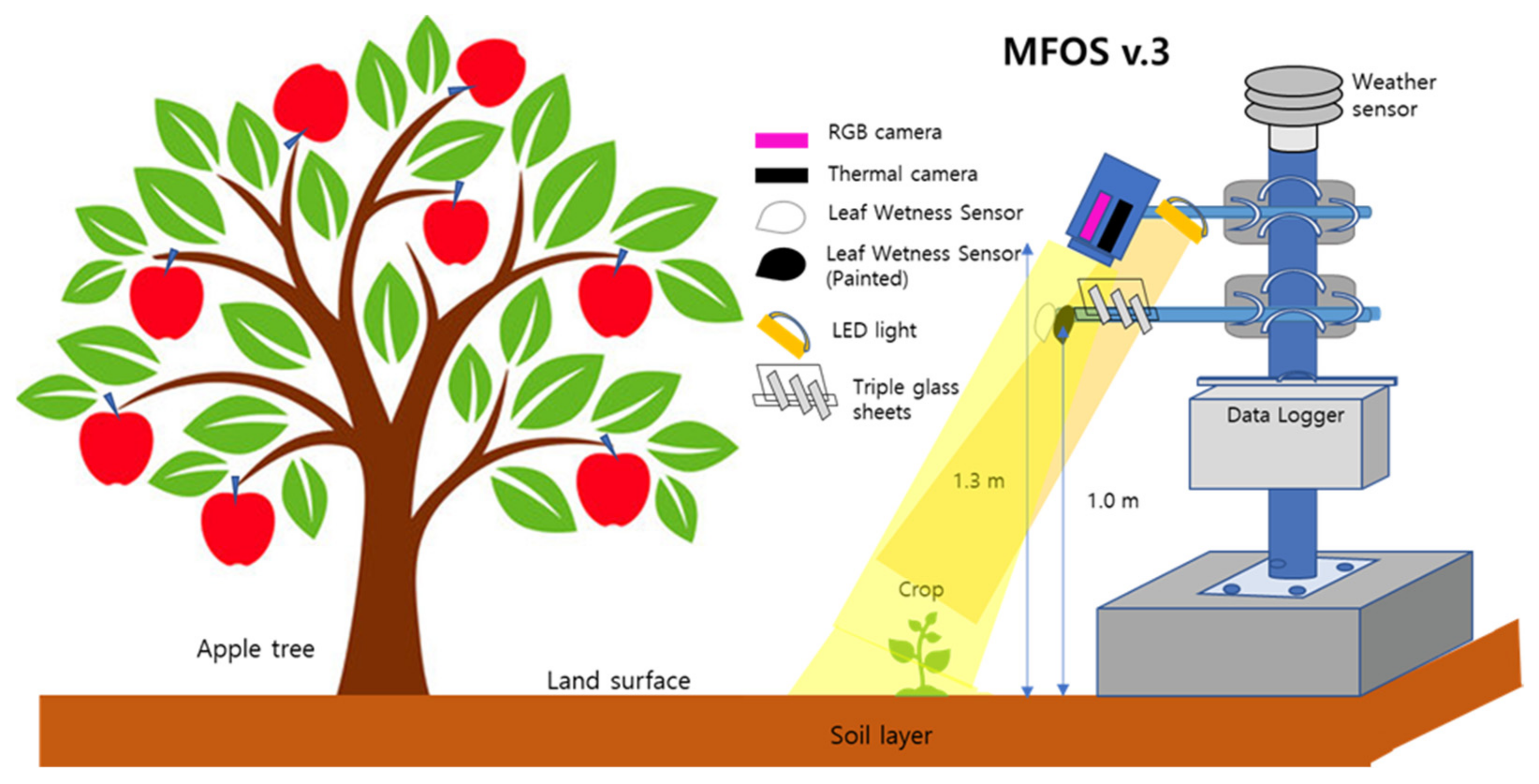
2.2. Observation System

The MFOS currently consists of seven components: a data logger, an RGB camera, a thermal infrared camera, a white-and-black LWS, LED lighting, and glass plates (Figure 2). The RGB and infrared cameras are positioned above the LWS so that the LWS is visible in the center of the image, while the ground surface and surrounding terrain features are also captured. The LWS was located approximately 1 m above the ground, and the two cameras were placed 1.3 m apart. Detailed specifications and descriptions of each sensor and tool are provided by Kim et al. in [11,12].

First, the RGB camera observes the ground and near-surface terrain features to determine the presence or absence of frost by directly identifying frosted spots in an image [10]. LED lighting connected to the data logger enables the observation of RGB images even under low-light conditions. The LED lights were automatically powered one minute before the camera started recording and turned off when the recording ended.

Second, the thermal infrared camera compensates for the inability to conduct observations with the RGB camera at dawn and at night. The two cameras used were an RGB camera (Raspberry Pi Camera V2.1, Beijing, China) on a microcomputer (Raspberry Pi 4, Raspberry Pi Foundation, Cambridge, UK) and a thermal infrared camera (Lepton 3.5, FLIR, USA) [11,12]. The pixel resolution of the RGB camera was 3280 × 2464, and that of the thermal infrared camera was 160 × 120. The LWS was set at a distance of 80 cm from the camera and at a 130° vertical angle, and photos of the apple fruits were taken horizontally, 1 m from the camera. The camera automatically captured pictures every 10 min between 04:00–07:00 LST (Local Standard Time) and 17:00–20:00 LST daily. A power management board (Witty Pi 3, UUGear, Prague, Czech Republic) was added to the system to allow it to be used in low-power environments in order to minimize power consumption.

Third, the LWS uses an electrode to detect water or ice on its dielectric sensing surface. In general, LWS voltage values below 274 mV indicate dry conditions, and those above 284 mV indicate wet conditions, with frost falling between these dry and wet conditions [13]. The LWS voltage changes according to the sensor surface state transitions from frost or dry to wet, from wet to dry, or from dry to ice [14]. Savage [14] demonstrated that frost can be detected when the voltage changes with the surface of the LWS: the voltage value switches rapidly from a wet-to-ice change to a dry-to-ice change, and falls between the voltage values of the dry and wet states.

Fourth, the glass plates aid in detecting frost through changes in the opacity. Because the surface of an LWS is typically white, white frost cannot be distinguished in RGB camera images. Three glass plates (76 mm × 26 mm × 1 mm) placed at the same height as the LWS were used, allowing us to determine the frost on the LWS by checking the frost on the glass plate surfaces. Adapted from Lei et al. [15], glass plates become transparent without frost and opaque in the presence of frost [12].

Finally, the black-painted surface aids the LWS in determining the presence of frost in conjunction with its white surface. Kim et al. [12] tested the effect of a black surface coating on the observation of voltage values of an LWS and found that the coating did not interfere with the observation of voltage values. However, for aged equipment, the increase in surface coating resulted in voltage values similar to those of an unused LWS. Compared with the white LWS, which reflects light in the visible region, the surface of the black-painted LWS was visible in the RGB image.

2.3. Extraction of MFOS Surface Temperature

2.3.1. Object Surface Temperature Calculation and Accuracy

The thermal infrared camera in the initial MFOS version stores RGB information per pixel through simple screen capture, which only provides information on whether an object’s surface temperature is higher or lower than the ambient temperature [11]. To improve this, we used the Python-based open-source Pure Thermal UVC Capture code provided by GroupGets (https://github.com/groupgets/purethermal1-uvc-capture (accessed on 19 May 2024)) to extract and analyze the specific temperature values per pixel [12]. The temperature extraction accuracy of the improved thermal infrared camera was evaluated by comparing it with the APOGEE non-contact surface temperature sensor installed at the National Center for AgroMeteorology (NCAM). The evaluation showed a high correlation coefficient (greater than 0.99) and a slope close to 1. The mean difference between the two sensors was −0.209 °C, and the standard deviation was 0.941 °C, indicating that our thermal infrared camera showed a higher surface temperature. However, the differences in these values between 04:00 and 07:00 were 0.162 °C and 0.900 °C, respectively, indicating that our thermal infrared camera showed a lower surface temperature. This difference was attributed to the temperature difference because the two sensors did not capture the same LWS [12].

2.3.2. Apple Surface Temperature

The location of an LWS is fixed, but the location of a crop changes as it grows. Therefore, an object detection algorithm is required to determine the exact point at which to extract the fruit surface temperature. The Mask R-CNN algorithm, a deep-learning-based object detection algorithm, is the most accurate and convenient and can be used if the training data are sufficient [15,16]. The training data were obtained from the Microsoft Common Objects in Context (MS COCO) dataset, available as an open-source dataset, and the model was trained based on these data. The COCO dataset, created by Microsoft, is an open-source resource with hundreds of thousands of images of everyday objects (e.g., people, bicycles, fruit) suitable for training. For apple object detection, we used a pre-trained model built with RGB images captured in the MFOS and MS COCO datasets (Figure 3). It output the detected object, the probability, the bounding box, and masking data.

The fruit tree used for object detection in this study was a ‘Fuji’ apple tree. Figure 4 shows a schematic of the surface temperature extraction process based on the boundary of an apple tree generated through object detection. First, the object was detected by applying the Mask R-CNN learning model to the RGB image. The second step was to develop the detected fruit trees’ boundaries accurately. The third step was to overlay the thermal image at the boundary location. Finally, the surface temperature of the 3 × 3 grid points within the boundary was extracted and averaged to account for the deviation in the surface temperature between the center and edge of the fruit object. Because individual apple fruits will each entail a different detection accuracy, three apple fruits were selected based on the accuracy and distance.

The resolution of the RGB image was 3280 × 2464 pixels, and that of the thermal infrared image was 160 × 120 pixels. The Mask R-CNN model, pre-trained with the COCO dataset, used training images with a resolution of 800 × 600 pixels. Therefore, the camera image-matching technique was practically important. To create apple fruit boundaries using the pre-trained model, we resized the RGB image to 800 × 600 pixels using the INTER_NEAREST resizing algorithm, which is a linear interpolation built into the Python package (OpenCV’s cv2.resize). The thermal infrared image was also resized to 800 × 600 pixels using the same algorithm. Next, the two resized images were matched by focusing them onto each other with horizontal image movement, because the horizontal distance between the two cameras was approximately 4 cm. Finally, the image boundary mismatch problem (small distortion and rotation error) around the object boundary was minimized by extracting 3 × 3 grid points located around the center of the apple fruit and calculating the average temperature.

2.4. Numerical Forecasting Models

The NCAM uses the Land–Atmosphere Modeling Package (LAMP) to conduct medium-range forecasts of the atmospheric and soil layers in order to support agriculture and forestry. LAMP/WRF uses UM data from the Korea Meteorological Administration and consists of four domains with grid intervals of 21,870 m (d01), 7290 m (d02), 2430 m (d03), and 810 m (d04). The model dynamics and physical processes follow those described in previous studies [17,18,19] and use 30 s resolution USGS data for domains one through three and 1/3 s resolution Korea Ministry of Environment land-cover data for domain four.

In this study, frost prediction with the LAMP/WRF model was performed by applying a frost point prediction equation (Equation (1)) to the model-predicted fields, and the model was started from three different initial times to allow estimations of its predictability. The specific frost-point temperature ($T_f$) is calculated as follows:

$$\begin{gathered} T_f=T_d+\Delta f, \\ \Delta f=p_1{T}_d^3+p_2{T}_d^2+p_d{T}_d^1+p_4, \end{gathered}$$

(1)

where $T_d$ is the model dew-point temperature, and $p_1$ = 0.000006, $p_2$ = −0.0003, $p_3$ = −0.1122, and $p_4$ = 0.1802, which are constants. If the difference between the 2 m model air temperature and the frost-point temperature is within ±1 °C, it is assumed that model frost occurred at that grid point at that time [20].

3. Results and Discussion

3.1. Preliminary Test: Evaluation of MFOS Surface Temperature

3.1.1. Apple Surface Temperature

An analysis was conducted to determine the temperature difference between the surface of the LWS (LWS1: unpainted surface, LWS2: black-painted surface) and the fruit in both rainfall and no-rainfall cases (Figure 5). This analysis spanned from 17:00 on 2 August 2022 to 20:00 on August 8, 2022. Precipitation occurred from 17:00 on 2 August to dawn on 4 August and from 07:00 on 7 August to 20:00 on 8 August. In the precipitation case, there was almost no difference between the surface temperature data of the LWS and the fruit tree; however, in the no-precipitation case, the difference between the LWS and the fruit tree data increased significantly from 17:00 to 20:00 and decreased almost constantly during the early morning. Correlation analysis was performed by dividing the data from 27 July to 28 October into four time periods—0–6, 6–12, 12–18, and 18–24—to investigate the feasibility of using an LWS to predict the surface temperature of fruit trees.

The correlation coefficients ranged from 0.9357 to 0.9948 for all hours of the observation period (Figure 6). A relatively low correlation coefficient of 0.9357 and a high Root-Mean-Squared Deviation (RMSD) of 2.8732 were found at 12–18 h compared with those found in the other hours; however, because the probability of frost occurrence was very low during these hours, the surface temperature prediction of the LWS for frost classification and prediction was not affected. Between 00:00 and 12:00, when frost is likely to occur, the surface temperatures of the apple fruits and LWS had a high correlation coefficient (>0.93), a low RMSD (<2.8732), and a slope close to 1. This indicates that the surface temperature of an LWS can be used to predict the surface temperature of apples.

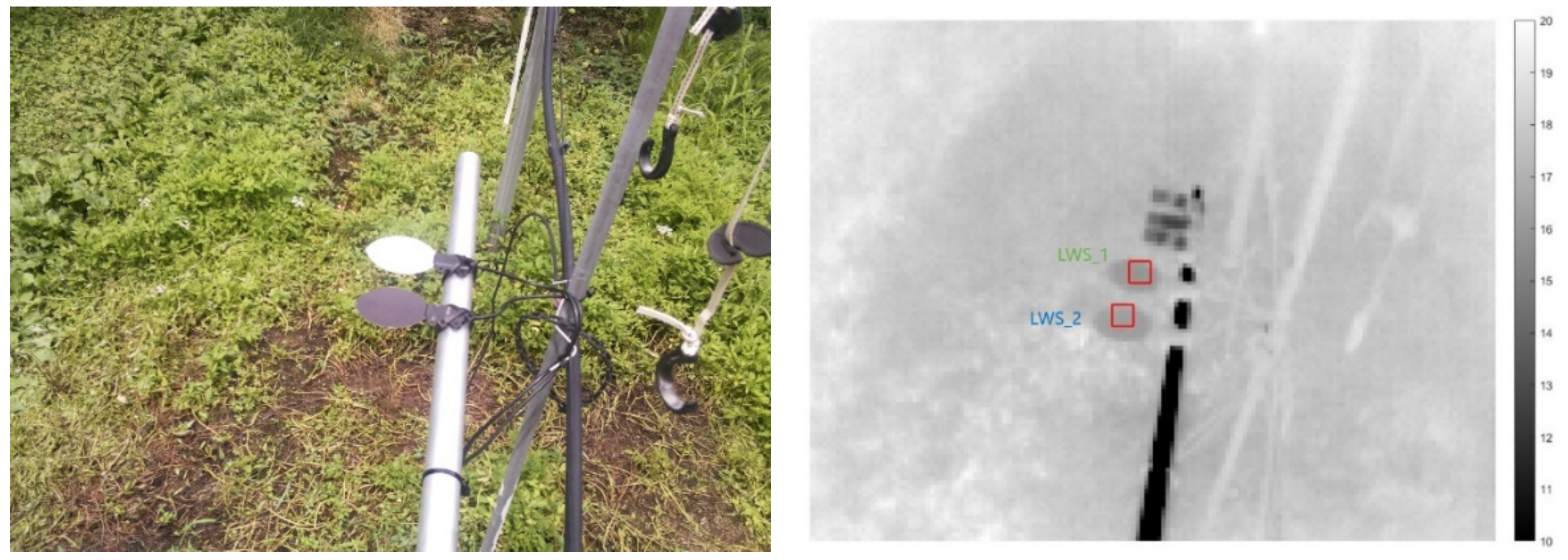
3.1.2. LWS Surface Temperature

The COCO dataset does not include any classes related to leaves in its list of supported classes. Therefore, in this study, we extracted leaf surface temperatures using manual settings (Figure 7).

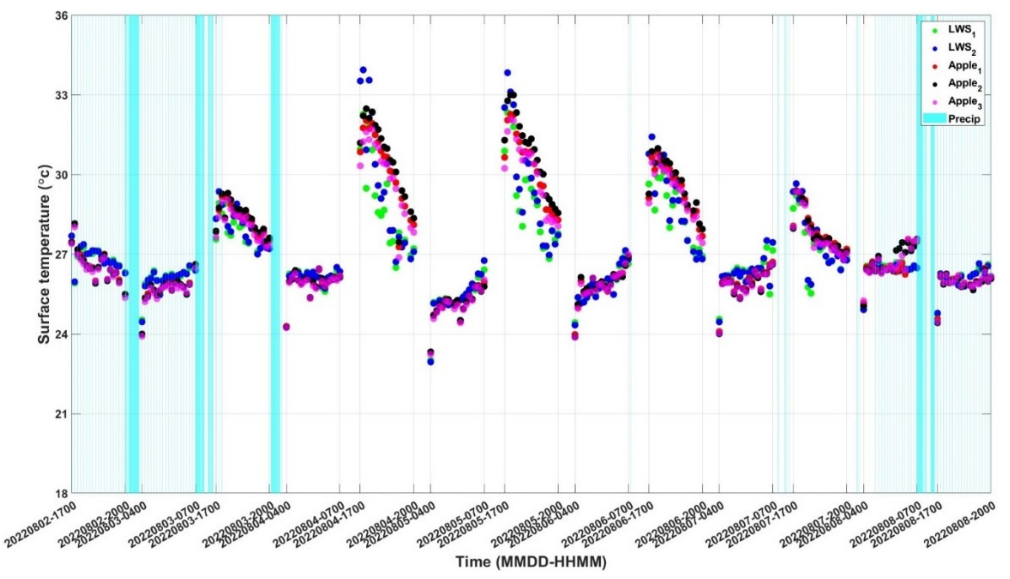
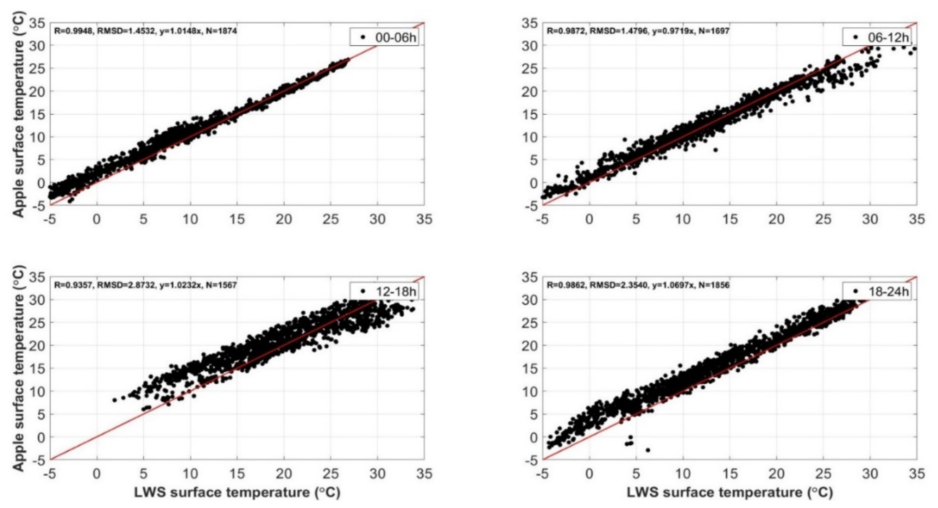
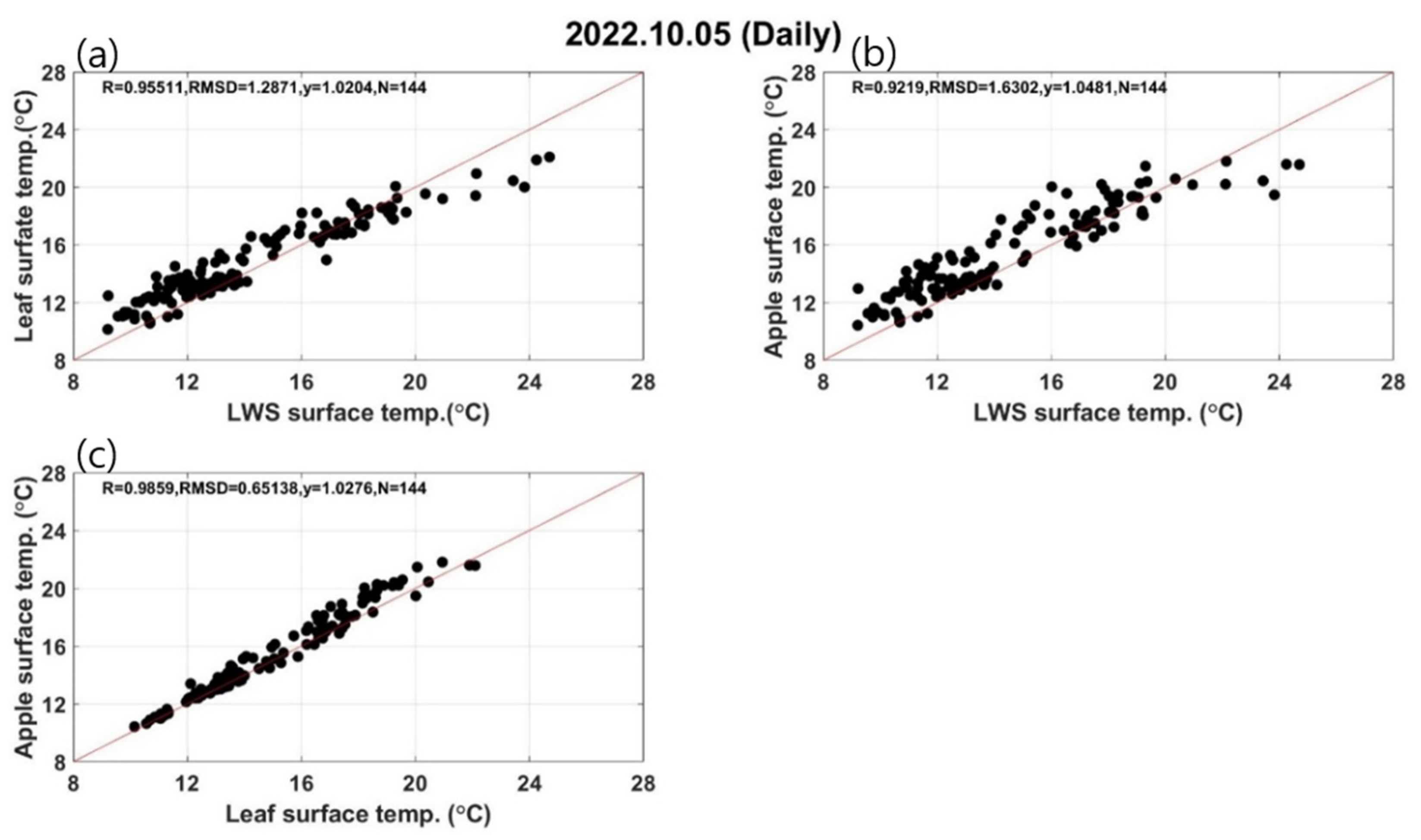
3.1.3. Comparison of Apple and LWS Surface Temperatures

Figure 8 shows the surface temperature data extracted by selecting a large leaf, which is easy to recognize as an object, on 5 October 2022, and comparing its temperature with the surface temperatures of apples and the LWS. Rainfall was detected by the rain sensor at 10:40 LST on this day, and an average temperature of 13.7 °C was observed. The surface temperatures of the leaves and LWS were highly correlated; however, the leaf temperature was slightly higher than that recorded by the LWS. The surface temperatures of the apples and LWS were similar, with a correlation coefficient of more than 0.92; however, the surface temperatures of the apples were higher. The surface temperatures of the apples and leaves showed the highest correlation coefficient (>0.98), the lowest RMSD, and a graph slope close to 1.

3.2. Actual Test: Evaluation of Frost Prediction Using MFOS

The two selected frost cases spanned from 12:00 LST on 17 October 2022 to 12:00 LST on 18 October 2022 (Case 1) and from 12:00 LST on 23 October 2022 to 12:00 LST on 24 October 2022 (Case 2). The frost prediction performance of the numerical model was analyzed for three different model initial times and two different model domains (d03 and d04). The model-predicted frost data were extracted at three points (pts1, pts2, and pts3) closest to the latitude and longitude of the study site on d03 and d04 and were compared with the observed data from the MFOS. An algorithm [21] was adopted to determine the water status on the LWS’s surfaces to confirm the frost occurrence using MFOS data. This algorithm uses the voltage and surface temperature of the LWS and classifies its surface state as dry, wet, or iced to determine whether frost has occurred.

3.2.1. Case 1 (18 October 2022)

Case 1 was an intense and persistent frost event; the features captured by the MFOS are shown in Figure 9. In the RGB camera image captured at 04:00 LST, frost formed on the black-painted LWS surface and the surrounding equipment, and the increased opacity of the three glass plates further confirmed the occurrence of frost. This frost was observed with the RGB camera until 08:00 LST and had melted entirely by 09:00 LST.

Figure 10 shows the time-series graphs of the MFOS observations and the LAMP/WRF model predictions for Case 1. For the period analyzed, the observations classified approximately 7 h of frost as occurring from 00:00 LST to 07:00 LST on Day 18 (blue shaded area in Figure 10). The more significant the difference between the time classified as frost in the observations and the initial time of the model, the more significant the difference between the air temperature and dew-point temperature in the model at the time of frost occurrence. In this case, the LAMP/WRF model with initial times of 09:00 LST on 9 October and 09:00 LST on 12 October did not predict the frost observed in the MFOS. The LAMP/WRF model with an initial time of 09:00 LST on 16 October did not predict frost in domain d03 because the difference between the air temperature and dew-point temperature was not very small. However, the model captured frost events in domain d04 at 06:00 and 07:00 LST (see the lower and right panels of Figure 10).

3.2.2. Case 2 (24 October 2022)

Case 2 was a weak and intermittent frost event, and the features captured with the MFOS are shown in Figure 11. Unlike in Case 1, the RGB camera could not confirm the occurrence of frost. The glass plate surfaces were somewhat contaminated, and their opacity had changed. This change is thought to be due to the condensation of dew on the glass plate surfaces caused by high relative humidity and temperatures below 0 °C at the time of the observation, classified as frost. This was classified as frost because the algorithm for determining the surface water condition of the LWS did not distinguish between frost generated by the sublimation of water vapor and that generated by frozen dew.

Figure 12 shows the time-series graphs of the MFOS observations and LAMP/WRF model predictions for Case 2. Approximately four hours of observations from 04:00 LST to 08:00 LST on 24 October 2022 were classified as frost (blue shaded area in Figure 12). The model with an initial time of 09:00 LST on 16 October 2022 predicted frost at all three locations (pts1, pts2, and pts3) in the evening, indicating temporal mismatches (earlier than the observed event). Moreover, the model with an initial time of 09:00 LST on 19 October 2022 did not predict frost. However, the model with an initial time of 09:00 LST on 23 October 2022 predicted frost in both d03 and d04, including all three locations, simultaneous to the observed frost (lower and right panels in Figure 10).

Cases 1 and 2 demonstrate that the MFOS can provide temporally high-resolution frost information and distinguish between persistent and intermittent frosts, which is extremely helpful for evaluating sub-hourly frost forecast models. For the persistent long-lived frost event at dawn on 18 October 2022, the LAMP/WRF model with an initial date of 16 October showed that the event was missed in d03 but was captured in d04, whereas the LAMP/WRF model missed it on 12 October, regardless of the domain. For the short-lived frost case at dawn on 24 October 2022, the LAMP/WRF model with an initial date of 23 October 2022 captured the frost signal with temporal mismatches in d03 (i.e., in the evening, not at dawn), whereas the LAMP/WRF model with an initial date of 19 October completely missed it. These results indicate that the closer the initial time of the model is to the actual time of the frost event, the better the prediction performance. In addition, they suggest that having higher resolution and more realistic land-cover data from d03 would be useful for frost prediction.

4. Summary and Concluding Remarks

This study introduces the MFOS and demonstrates its potential for remote-sensing-based fruit and leaf temperature extraction. It also evaluates model-predicted frost-point temperatures for low-temperature cases in apple orchards. The MFOS v3 uses an LWS (with both a conventional white surface and a new black one), an RGB camera, a thermal infrared camera, triplet glass plates, and LED lighting to automatically capture high-resolution images, detect fruit and leaf objects, and extract their surface temperatures.

(1)

Installing and operating this system in an apple orchard confirmed that the accuracy and efficiency of the automatic frost observation improved for both weak and robust frost events, thereby enhancing the usefulness of this observation system as an input for frost prediction models.

(2)

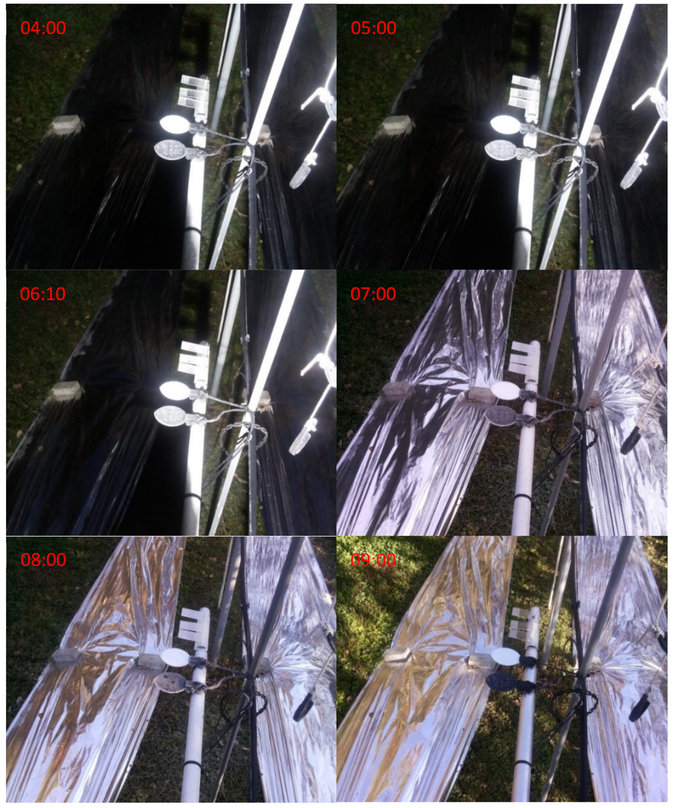
Resolution matching of the RGB and thermal infrared images was performed by resizing the images, matching them through horizontal movement, and conducting apple-centered averaging.

(3)

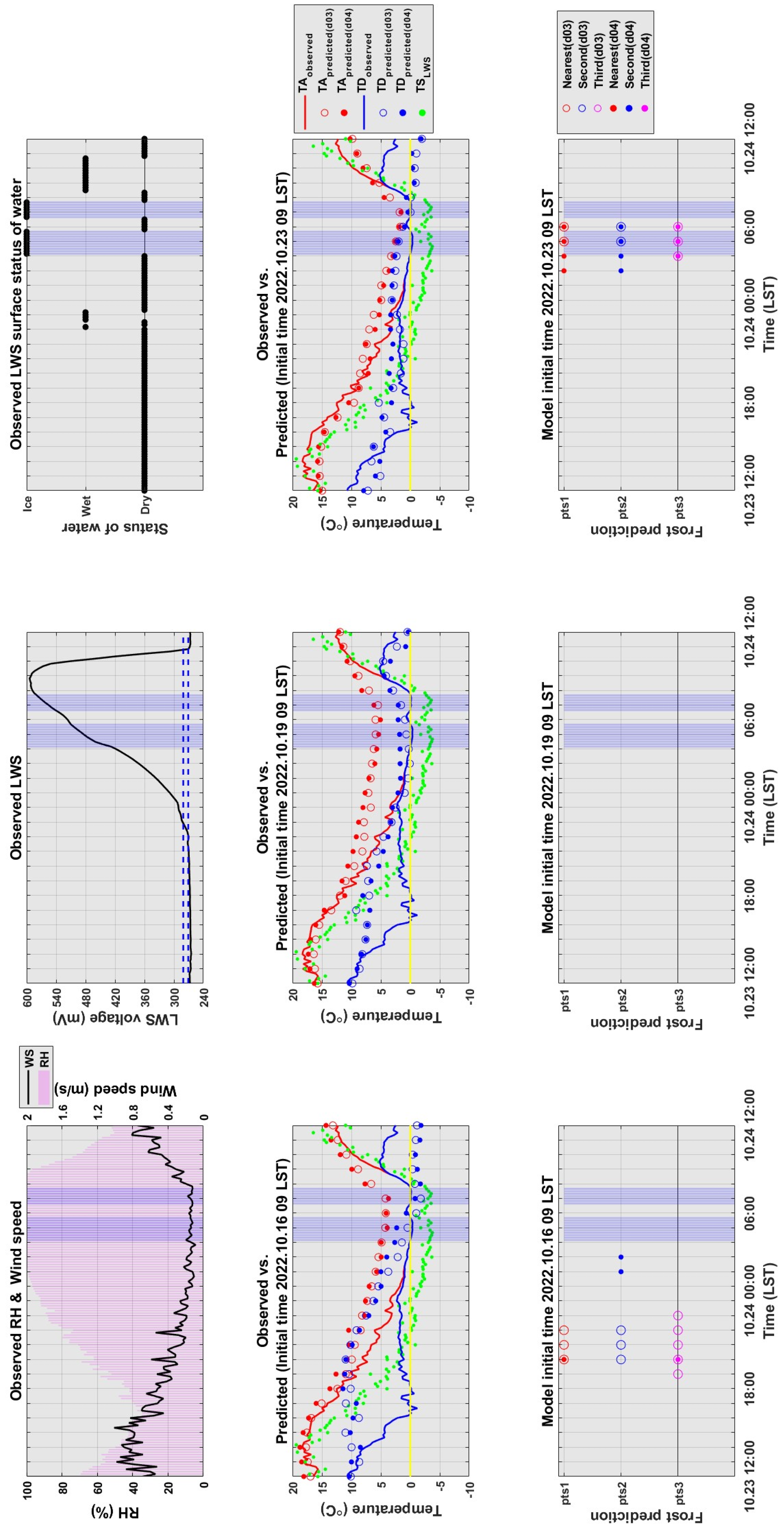
An evaluation of the frost forecast results from the LAMP/WRF numerical model showed that frost forecast evaluations could be conducted hourly, and the model could be validated in a shorter time by increasing its output frequency.

(4)

When objects were partially obscured by obstacles such as leaves, the accuracy significantly decreased, leading to failure in object detection. Unlike fruits, the wind sways tree leaves, and their position changes considerably depending on the time of image capture, resulting in relatively low accuracy in surface temperature estimation. Further research should be conducted on this topic, which will help in developing techniques for measuring the temperatures of various parts of crops.

Because the selected frost cases are only two examples, the use of the MFOS in many other frost case analyses is expected to lead to new and detailed findings in frost observation and aid in developing a temporally high-resolution frost warning model in the future. We plan to carry out the following:

(1)

To observe fruit tree surface temperatures in summer to examine the applicability of the studied system in high temperatures, such as during heat waves;

(2)

To upgrade the classification algorithm to estimate the surface temperatures of fruit trees using LWS and observe fruit damage from low and high temperatures;

(3)

To keep producing image (and video) observations for use in frost prediction models, and include them in a database;

(4)

To improve the representation of surface vegetation in the numerical weather model so that orchard farms can be more realistically implemented (e.g., [22]).

References

1. Noh, I.S.; Doh, H.-W.; Kim, S.-O.; Kim, S.-H.; Shin, S.E.; Lee, S.-J. Machine learning-based hourly frost-prediction system optimized for orchards using automatic weather station and digital camera image data. Atmosphere 2021, 12, 846. [Google Scholar] [CrossRef]
2. Rodrigo, J. Spring frosts in deciduous fruit trees—Morphological damage and flower hardiness. Sci. Hortic. 2000, 85, 155–173. [Google Scholar] [CrossRef]
3. Korea Meteorological Administration (KMA). Abnormal Climate Report; KMA: Seoul, Republic of Korea, 2019.
4. Korea Meteorological Administration (KMA). Ground Meteorological Observation Guidelines; KMA: Seoul, Republic of Korea, 2022.
5. Groh, J.; Slawitsch, V.; Herndl, M.; Graf, A.; Vereecken, H.; Pütz, T. Determining dew and hoar frost formation for a low mountain range and alpine grassland site by weighable lysimeter. J. Hydrol. 2018, 563, 372–381. [Google Scholar] [CrossRef]
6. Goswami, J.; Sharma, V.; Chaudhury, B.U.; Raju, P.L.N. Rapid identification of abiotic stress (frost) in in-filed maize crop using UAV remote sensing. Int. Arch. Photogramm. Remote Sens. Spat. Inf. Sci. 2019, 42, 467–471. [Google Scholar] [CrossRef]
7. Tait, A.; Zheng, X. Mapping frost occurrence using satellite data. J. Appl. Meteorol. 2003, 42, 193–203. [Google Scholar] [CrossRef]
8. Wang, S.; Chen, J.; Rao, Y.; Liu, L.; Wang, W.; Dong, Q. Response of winter wheat to spring frost from a remote sensing perspective: Damage estimation and influential factors. ISPRS J. Photogramm. Remote Sens. 2020, 168, 221–235. [Google Scholar] [CrossRef]
9. Valjarević, A.; Filipović, D.; Valjarević, D.; Milanović, M.; Milošević, S.; Živić, N.; Lukić, T. GIS and remote sensing techniques for the estimation of dew volume in the Republic of Serbia. Meteorol. Appl. 2020, 27, e1930. [Google Scholar] [CrossRef]
10. Noh, I.S.; Lee, S.-J.; Lee, S.Y.; Kim, S.-J.; Yang, S.-D. A High-Resolution (20 m) Simulation of Nighttime Low Temperature Inducing Agricultural Crop Damage with the WRF–LES Modeling System. Atmosphere 2021, 12, 1562. [Google Scholar] [CrossRef]
11. Kim, S.H.; Lee, S.-J.; Son, S.W.; Cho, S.S.; Jo, E.S.; Kim, K.R. Unmanned Multi-Sensor based Observation System for Frost Detection—Design, Installation and Test Operation. Korean J. Agric. For. Meteorol. 2022, 24, 95–114. [Google Scholar]
12. Kim, S.H.; Lee, S.-J.; Kim, K.R. Improvement of Multiple-sensor based Frost Observation System (MFOS v2). Korean J. Agric. For. Meteorol. 2023, 25, 226–235. [Google Scholar]
13. Campbell Scientific. LWS: Dielectric Leaf Wetness Sensor Instruction Manual; Revision 11/18; CSI: Ogden, UT, USA, 2018; p. 19. Available online: http://s.campbellsci.com/documents/us/manuals/lws.pdf (accessed on 2 May 2024).
14. Savage, M.J. Estimation of frost occurrence and duration of frost for a short-grass surface. South Afr. J. Plant Soil 2012, 29, 173–187. [Google Scholar] [CrossRef]
15. Zhu, L.; Cao, Z.; Zhuo, W.; Yan, R.; Ma, S. A new dew and frost detection sensor based on computer vision. J. Atmos. Ocean. Technol. 2014, 31, 2692–2712. [Google Scholar] [CrossRef]
16. Chu, P.; Li, Z.; Lammers, K.; Lu, R.; Liu, X. Deep learning-based apple detection using a suppression mask R-CNN. Pattern Recognit. Lett. 2021, 147, 206–211. [Google Scholar] [CrossRef]
17. Lee, S.-J.; Kim, J.; Kang, M.S.; Malla-Thakuri, B. Numerical simulation of local atmospheric circulations in the valley of Gwangneung KoFlux sites. Korean J. Agric. For. Meteorol. 2014, 16, 246–260. [Google Scholar] [CrossRef]
18. Song, J.; Lee, S.-J.; Kang, M.S.; Moon, M.K.; Lee, J.-H.; Kim, J. High-resolution numerical simulations with WRF/Noah-MP in Cheongmicheon farmland in Korea during the 2014 special observation period. Korean J. Agric. For. Meteorol. 2015, 17, 384–398. [Google Scholar] [CrossRef]
19. Lee, S.-J.; Song, J.; Kim, Y.J. The NCAM Land-Atmosphere Modeling Package (LAMP). Version 1: Implementation and Evaluation. Korean J. Agric. For. Meteorol. 2016, 18, 307–319. [Google Scholar] [CrossRef]
20. Gultepe, I.; Zhou, B.; Milbrandt, J.; Bott, A.; Li, Y.; Heymsfield, A.J.; Ferrier, B.; Ware, R.; Pavolonis, M.; Kuhn, T.; et al. A review on ice fog measurements and modeling. Atmos. Res. 2015, 151, 2–19. [Google Scholar] [CrossRef]
21. Kim, K.R.; Jo, E.S.; Ki, M.S.; Kang, J.H.; Hwang, Y.J.; Lee, Y.H. Implementation of an Automated Agricultural Frost Observation System (AAFOS). Korean J. Agric. For. Meteorol. 2024, 26, 63–74. [Google Scholar]
22. Lee, S.J.; Berbery, E.H.; Alcaraz-Segura, D. Effect of implementing ecosystem functional type data in a mesoscale climate model. Adv. Atmos. Sci. 2013, 30, 1373–1386. [Google Scholar] [CrossRef]
Figure 1. Study area and observation system installation site: (a) Location of the observation site and surrounding terrain. (b) Multiple-sensor-based frost observation system (MFOS) field site.
Atmosphere 15 00906 g001
Figure 2. Multiple-sensor-based frost observation system (MFOS) version 3. The previous version was MFOS v2 (refer to [1,11,12]) and meteorological sensor data is transmitted to the NCAM PC or server through the wireless communication function of the MFOS data logger.
Atmosphere 15 00906 g002
Figure 3. Post-processing workflow for detecting apple objects with a pre-trained model.
Atmosphere 15 00906 g003
Figure 4. Extracting the fruit surface temperature (°C) from a multiple-sensor-based frost observation system (MFOS) infrared image produced in an apple farm. The left side shows the RGB camera image and the right shows the thermal camera image. We applied the bounding box extracted from the RGB camera on to the thermal image and calculated the 9-point average temperatures.
Atmosphere 15 00906 g004
Figure 5. Comparison of the surface temperatures of apples and the leaf wetness sensor (LWS) for the period of 17:00 LST 2 August 2022 to 20:00 LST 8 August 2022. The surface temperature data were extracted from a thermal infrared camera image according to [11].
Atmosphere 15 00906 g005
Figure 6. Correlation analysis of the surface temperatures of apples and the leaf wetness sensor (LWS) for the period of 27 July 2022 to 28 October 2022. The surface temperature data were extracted from a thermal infrared camera image according to [11]. (R: correlation coefficient, RMSD: Root-Mean-Squared Deviation, y: regression equation, N: number of samples.)
Atmosphere 15 00906 g006
Figure 7. The process of extracting the leaf wetness sensor’s surface temperature.
Atmosphere 15 00906 g007
Figure 8. Comparison of surface temperatures (a) between apple leaves and the leaf wetness sensor (LWS), (b) between apple fruit and the LWS, and (c) between apple fruit and apple leaves in the orchard during the day on 5 October 2022. The surface temperature data were extracted from a thermal infrared camera image [11].
Atmosphere 15 00906 g008
Figure 9. RGB camera images from 04:00 LST to 09:00 LST on 18 October 2022 (Case 1).
Atmosphere 15 00906 g009
Figure 10. Comparison of observations and model predictions for a frost event (Case 1) from 12:00 LST on 17 October 2022 to 12:00 LST on 18 October 2022. The observations were made at an altitude of approximately 2 m, and the model predictions were also set at 2 m. pts1, pst2, and pst3 refer to the grid points closest, second closest, and third closest to the observations in two domains (d03 and d04), respectively. (TAobserved: observed air temperature, TApredicted: air temperature according to the numerical model, TDobserved: observed dew-point temperature, TDpredicted: dew-point temperature according to the numerical model, TSLWS: surface temperature according to the leaf wetness sensor (LWS). The blue range shows the section where the LWS surface was classified as ice in the observation through the algorithm).
Atmosphere 15 00906 g010
Figure 11. RGB camera images from 04:00 LST to 07:00 LST on 24 October 2022 (Case 2).
Atmosphere 15 00906 g011
Figure 12. Same as Figure 10 but for the Case 2 from 12:00 LST on 23 October 2022 to 12:00 LST on 24 October 2022.
Atmosphere 15 00906 g012
Disclaimer/Publisher’s Note: The statements, opinions and data contained in all publications are solely those of the individual author(s) and contributor(s) and not of MDPI and/or the editor(s). MDPI and/or the editor(s) disclaim responsibility for any injury to people or property resulting from any ideas, methods, instructions or products referred to in the content.