Abstract
Tornado outbreaks (TOs) are highly dangerous meteorological phenomena common in the United States and have limited known relationships with climate variability. Many of the challenges in understanding TOs result from a lack of formal TO quantification (both in definition and impact). Here, we present a TO definition based on a spatially cohesive and distinct region of tornado activity and present a TO intensity index using tornado characteristics within the TO region. In developing this index, we present a support vector regression-based detrending methodology to remove the secular trends within tornado reporting. The resulting TO definition suggests a decline in TO activity of roughly 1 TO per 4–5 years, with a similar decline in TO intensity. In addition, the relationship between this new quantification of TOs and common North American interannual and monthly climate variability indices is explored, namely the El Niño Southern Oscillation, the North Atlantic Oscillation, the Arctic Oscillation, and the Pacific North American Oscillation. In general, the links between these teleconnections and TO frequency and intensity were minimal (and sometimes in opposition when comparing TO frequency and intensity), but interesting patterns emerged that may offer an initial pathway to exploring longer-term TO predictability.
1. Introduction
Outbreaks of severe weather (including tornadoes) are notoriously challenging to link to climate-scale phenomena, owing to the relative lack of an objective definition of an outbreak and numerous issues with quantifying outbreak impacts. However, these events, particularly those that produce multiple tornadoes (known as tornado outbreaks [TOs]), are critical hazards for regions east of the Mississippi River in the United States. Despite some efforts to quantify the relationship between outbreaks and climate-scale phenomena [1,2,3], no work has directly explored the relationship between TO intensity and natural interannual variability that impacts North America.
Early TO studies [4,5,6,7,8] were the first to explore defining a TO. These studies all had similarities, but the work never yielded an agreed upon definition for a TO. Instead, they utilized varying definitions, discussing multiple tornado occurrences [4,5,6], days of tornado activity in which the activity was “unusually large” [7], and eventually a distinct criterion of 10 or more tornadoes within one group on a given tornado day [8]. Another study explored categorizing outbreaks based on the number of tornadoes [9], which was a first effort at sorting TOs by intensity and impact, rather than categorizing events as TO or non-TO. More recent work, using the TO definition of six or more tornadoes associated with a single synoptic-scale system, explored meteorological characteristics of TOs [10], and [11] made the first effort to develop an index that could rank outbreaks by relative intensity among all severe weather modes (tornadoes, wind, and hail). This summary is far from an exhaustive list of the evolution of the TO definition, which is specified in detail in [12] and demonstrates that, to date, no consistent TO definition exists. As such, most studies typically reference the American Meteorological Society TO definition of “multiple tornado occurrences with a particular synoptic-scale system” [13]. The dubious nature of the TO definition remains an important challenge when linking TOs to climate-scale variability, an issue this study seeks to address.
While the challenges associated with defining an outbreak remain clear, even fewer studies have explored the intensity of these outbreaks (typically quantified through outbreak impacts), and any climate-related shifts in outbreak intensity have remained difficult to identify. Some studies have explored the problem of quantifying outbreak intensity, including [9,11], which were discussed earlier. More recent studies [14,15] expanded on the work of [11] by utilizing characteristics of the storm impacts tied to the outbreak event. Specifically, in [14], the authors developed an index for ranking severe weather outbreak intensity based on storm report characteristics obtained from the United States National Oceanic and Atmospheric Administration’s (NOAA’s) Storm Prediction Center storm report database [16], an actively updated impact database of the three main severe weather event hazards (tornadoes, wind, and hail). Their study was the first effort to develop a multivariate index for ranking severe weather reports, but it encompassed all report types (it was not just limited to tornadoes or TO events). As expected, they accurately identified tornadoes as the most impactful severe weather hazard associated with outbreaks, and their index ranked TOs as the highest severity among the outbreaks they considered. An important limitation of their study was the lack of a formalization of the region of the outbreak, which was instead categorized by the spatial spread of reports using their defined “middle 50% parameter”. The work in [15] sought to improve upon this limitation by utilizing spatial kernel density estimation from the severe weather reports, which in turn would reveal spatially cohesive regions of report activity, serving as a useful proxy for outbreak impact regions. As in [14], the work in [15] was not just confined to TOs, and their resulting rankings have not been updated since the publication of the work in 2011. A more recent study [17] developed an outbreak intensity measure specifically for TOs, known as “adjusted Fujita miles”, which utilizes integrated path length and EF scale rating [18]. This measure provides another useful quantification of outbreak intensity that differs from those in [14,15] but offers similar rankings for the most impactful TO events.
Despite these considerable advances, there remain two key outstanding challenges regarding TO climatology, namely the lack of a formal TO definition and the absence of a consistent methodology for quantifying TO intensity (i.e., [14,15] versus [17]). Here, we present an outbreak intensity scheme that blends the methods of [14,15] and [17] into an updated quantification of TO intensity and formalize a TO definition using the kernel density estimation approach of [15]. We then explore monthly and annual TO frequency and intensity and relate these quantities to interannual and monthly variability indices relevant to North America, including the El-Niño Southern Oscillation (ENSO—[19,20]), the North Atlantic Oscillation (NAO—[21]), the Pacific–North American pattern (PNA—[21]), and the Arctic Oscillation (AO—[22]). We hypothesize that statistically significant relationships between our updated TO intensity index and these interannual variability patterns will exist, and we expect that these relationships will offer insight into the predictability of higher or lower-intensity outbreak seasons in future studies. Section 2 overviews the data and methods utilized herein, while Section 3 presents the results. Section 4 provides a summary and conclusions.
2. Data and Methods
2.1. Datasets
The methods utilized in [14,15,17] relied heavily upon the SPC storm report database [16], the top global severe weather report database. The data are updated annually and are available from 1950 to 2022, with data for future years forthcoming pending validation. Owing to data availability at the onset of this study and the questionable nature of reported data prior to 1960, we limited our study period to 1960–2021 (62 years). The database includes numerous subcategories of severe weather report characteristics for each of the three primary severe weather modes (tornadoes, wind, and hail), where these subcategories describe characteristics of individual severe weather reports (e.g., hail size, max wind speed, tornado path length, etc.). As this work contrasts that of [14,15] by focusing exclusively on TOs, we will be only utilizing the tornado report characteristics in this study. These tornado report characteristics include the EF scale, path length and width, report time and location, injury and fatality counts, and estimated damage losses in dollar amounts. As societal-based parameters (injuries, fatalities, and damage estimates) are highly correlated with the location of the outbreak (i.e., if the outbreak impacts a highly populated area), they are not necessarily directly relevant to assessing the meteorological intensity of a TO (as opposed to societal impact). Thus, we only retained path length and width, as well as the EF scale, to characterize tornadoes in our study. An example of plotted tornado reports from the database for the major 27 April 2011 tornado outbreak that impacted the southeastern United States is provided in Figure 1. Additional outbreak-scale-derived parameters were computed from these variables as well, as we discuss below.
In addition to the storm report data utilized for building the TO intensity index, we also required a time series of the seasonal interannual variability indices for the four primary patterns considered herein. To quantify the ENSO phase and magnitude, we utilized the Oceanic Niño index ONI—[19,20] provided by NOAA’s Climate Prediction Center (CPC—[23]). This index characterizes the ENSO phase using 3-month running means of SST anomalies in the Niño 3.4 region [19]. We utilized CPC’s definition for each ENSO phase, and we compared the ONI against the annual TO frequency and intensity to quantify interannual variability relationships.

Figure 1.
The tornado reports from the SPC storm report database for the major TO of 27 April 2011. Each red line/point corresponds to a tornado report with EF scale attached. The image was generated using Severe Plot [24], available from the SPC. Note that only the tornado report data are provided despite the event consisting of multiple severe weather types.

For the remaining variability indices, which are derived from either 500 hPa (NAO and PNA) or 1000 hPa (AO), we used the monthly databases provided by the CPC. These time series were compared with monthly counts and average intensity index values to quantify the relationships between the natural variability structures in the geopotential height and SST fields and TO intensity. This offered a monthly relationship between highly variable teleconnections and monthly TO intensity/frequency, as discussed below.
2.2. Methods
2.2.1. Defining a TO
As stated previously, no formal TO definition exists. For our study, a TO definition that can also be used to quantify TO intensity is required. Thus, we developed a TO definition that allowed for outbreaks to be spatially distinct (as in [14,15]) and to be characterized by their net intensity (as in [14,17]). To identify spatially distinct regions of tornado activity that could be used to define a TO, it was first necessary to decompose the daily tornado reports into spatial outbreak regions following the methodology of [15]. Specifically, we utilized a Gaussian kernel density estimation (Equation (1)):
where h is a bandwidth (h = 1 in our study, following [15]). The approach requires constructing a grid xi underlying the analysis and computing the spatial distances between the observation and the grid. In our study, a grid spacing of 0.25° was used, though our outbreak region structures were similar to those in [15], who used 1°. We elected to use the smaller grid, owing to the lower density of observations in our study (which only considered tornado reports) versus [15] (which considered tornadoes, wind, and hail). Finally, like [15], we considered multiple contour values to define a KDE TO region (e.g., Figure 2), and we chose to utilize a contour of 0.002, as it presented similar outbreak region structures to those seen in [15], while avoiding the creation of one-tornado outbreak regions (e.g., Figure 2).
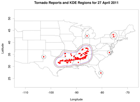
Figure 2.
KDE region alongside tornado reports for the morning of 27 April 2011 (precursor to the major TO later that day). Black contours represent a threshold of 0.001, while red represents 0.002 and blue 0.003. The red contours revealed a small outbreak region in NY alongside the main outbreak region. A threshold of 0.001 identified many single tornado reports as outbreaks, which was not desirable.
This KDE approach yielded one (or multiple) spatially distinct outbreak regions on a given tornado day that were categorized as individual TOs. Importantly, the density threshold of 0.002 limited the number of “outbreaks” that contained only a single tornado report (e.g., the discrete reports outside the contoured region in Figure 2). However, this issue did exist for some tornado days, so we also computed the annual median tornado count for every KDE-derived TO region. These annual median counts showed a notable step function transitioning from 1 tornado to 2 tornadoes after 1990 (with a few exceptions, not shown). This shift from 1 to 2 tornado reports demonstrates a secular shift in reporting data, but the use of the median avoided influence from major outlier events such as the 2011 outbreak season. Using this annual median, we defined a TO as an enclosed KDE tornado report region whose total tornado report count exceeded its median annual tornado report count. This definition ensured fewer than 50% of all KDE regions each year were considered TOs. As a result, in our early study years (pre-1990 primarily), a TO was defined as 2 or more tornado reports in a KDE region, while most years post-1990 defined a TO as 3 or more tornado reports. These criteria are quite minimal, which ensures a robust sample size (6723 TOs) from which we can derive outbreak intensity and frequency.
Once the TO regions were obtained, we computed several diagnostic variables from the SPC storm reports database that characterize the TO intensity, including the following:
- Number of tornadoes—the total count of tornadoes in the given outbreak;
- Number of EF0 and EF1 tornadoes (weak tornadoes);
- Number of EF2 and EF3 tornadoes (strong tornadoes);
- Number of EF4 and EF5 tornadoes (violent tornadoes);
- Total adjusted Fujita miles (AFM), computed following [17] for the TO.
While other studies have employed different quantities (total path length, the number of long track tornadoes, etc.), the AFM measure was shown in [17] to account for these properties of TOs. To ensure that some TO characteristics are not unnecessarily heavily weighted in the index, we elected to use AFM to account for these outbreak characteristics. This database of diagnostic variables for each TO was used to create a TO intensity index.
2.2.2. Detrending TO Diagnostic Variables
A known bias within the SPC storm report database is notable, statistically significant secular trends in annual means that exist within many of the outbreak diagnostic variables [25]. These trends resulted from reporting biases and the evolution of reporting technology throughout the study period. In prior studies [11,14], these annual means were detrended using a linear and exponential trend analysis. These detrended means were used to compute z-scores [14] on each TO diagnostic and summed to obtain an intensity index. While total, wind, and hail report counts in [14] showed the sharpest trends (not used herein), some diagnostics used in our study showed these secular trends as well. Most notably, the total tornado reports (Figure 3) show an upward trend, with a flattening of the mean outbreak total tornado counts in the final decade of the study period. In this example, the linear and exponential fits (as used in [11,14]) capture the initial years of the study well, but both trend lines diverge from the observed tornado report count trend in the final years of the time series, suggesting these methods do not characterize the full time series well. Total weak tornadoes, which have a similar time series to total tornado reports as they occur most frequently, also showed this divergent split between the exponential fit and the observed trend (not shown). Interestingly, the same shapes of trends were apparent in the annual standard deviations of the total tornado reports per TO and total weak tornado reports per TO. These secular trends suggest not only more observed weak tornadoes over time, but also more variability in those observations, both of which will have detrimental impacts on quantifying TO intensity fairly across the study period. Thus, we needed a new detrending strategy to remove secular biases, within both the mean and standard deviation of these two diagnostics.
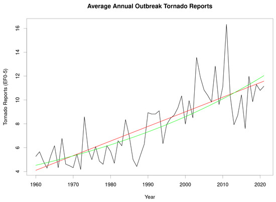
Figure 3.
Total tornado counts per TO for the study period, along with a linear trend line (red) and an exponential trend line (green). Note that tornado activity shows a relative flattening post-2000 (except for the anomalous 2011 season), but that both trend lines are inferring continued increases in tornado activity per outbreak.
To address the limitations resulting from previously employed detrending methods, we used a support vector regression (SVR—[26])-derived detrending approach for these two variables. SVR is a well-known machine learning technique that can be used to quantify nonlinear relationships (including temporal trends) within datasets. However, SVR has an advantage over nonlinear functions such as an exponential function, as it is adaptable, meaning that the same SVR model could be used for future years when employing the intensity index methodology described herein. This is an important utility of the SVR method, as a secondary goal of the outbreak intensity methodology would be to continuously update the indices on future years to diagnose changes, if any, in outbreak relationships with climate variability.
SVR utilizes a kernel map function to project data that show inherent nonlinear separability into a higher-dimensional hyperspace where linear separability may be attained. Several kernel maps exist, but the most utilized map function is the radial basis function (RBF—Equation (2)).
The RBF is based on a Gaussian function and utilizes a separation tuning parameter γ. Additionally, SVR utilizes quadratic programming optimization to obtain a linear fit that minimizes error with a tolerance threshold ε, which is also selected by the user. The optimization routine also weights points near the separation line at varying levels based on a penalty cost function C, another user-defined tuning parameter. In our study, we held the error tolerance constant at 0.01, which yielded a visually strong fit without overfitting the trend, and we tested values of C of 1, 10, 100, and 1000, as well as γ values ranging from 0.01 to 0.5. The configuration that yielded an improved R2 that did not show clear overfitting of the trend through visual inspection was retained (Figure 4). This was a subjective decision, but the sensitivity of the SVR curves to different values of γ and costs was minimal compared to the adjustments in ε. The SVR configurations used for each diagnostic are provided in Table 1 below.
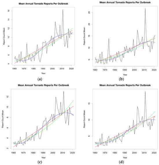
Figure 4.
Four diagnostics prior to detrending (those in Table 1) with trend lines for a linear trend (red), exponential trend (green), and SVR (blue). Panel (a) corresponds to the annual mean TO report count, while panel (b) corresponds to the annual TO report count standard deviation. Panels (c,d) are the same as (a,b), but for weak tornado report counts.

Table 1.
SVR configurations for four detrended variables used in this study. We also provide the R2 values for the linear, exponential, and SVR trend fits for each variable for comparison purposes. Note that SVR offers the highest R2 fit of any of the detrending methods employed.
2.2.3. Quantifying TO Intensity from Diagnostic Variables
After applying the detrending methods to the TO count diagnostics listed in Table 1, we computed z-scores on all 5 diagnostic variables listed in Section 2.2.1 using either the baseline annual mean and standard deviation (in the case of strong and violent tornado counts and AFM) or the SVR-detrended annual mean and standard deviations (Table 1). These five z-scores were then averaged (using equal weights) for each TO to calculate a total intensity index. Note that while [14] utilized multiple weighting schemes for their intensity index calculation, z-scores already provided larger magnitudes for anomalous diagnostic variable magnitudes, and the additional weight adjustments led to emphasizing and deemphasizing different TO diagnostics (depending on the weighting scheme). Importantly, these indices can be sorted in decreasing order of intensity to yield a TO ranking by intensity (similar to the research objectives of [14]). As a final step, each TO intensity index was averaged for a given study year to obtain the mean TO intensity by year. These values quantify annual TO intensity changes for the purposes of comparing with interannual variability metrics such as ENSO. We also computed monthly mean TO intensity to compare monthly variability with the NAO, PNA, and AO indices, which vary on much shorter time scales. Finally, we also computed total TO frequency by year and by month. We present the results from the intensity index below, as well as the climate-scale relationships between TO activity and interannual/monthly variability.
3. Results
3.1. Intensity Index Results
Some patterns in the resulting intensity indices (Figure 5a) were seen in prior studies [11,14], including a stark decrease in the index values for the top-10-ranked TOs and minimal variability in index changes for most TOs. The clear gamma-distributed shape of TO indices within each year (e.g., 2011 in Figure 5b) is presented as well.
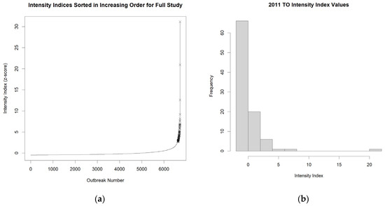
Figure 5.
Intensity indices for all 6723 TOs in this study (a) and an example of intensity index distribution for the 2011 TO season (b). The top 100 TO intensity indices in panel (a) are marked with an x symbol to denote their position in the distribution, as well as to reveal the heavily left-skewed nature of the intensity index (curve in panel (a)).
The top three outbreaks were clearly set apart from the remaining events (Figure 5a). These top three events included the 3 April 1974 “Super Outbreak” [27,28] (intensity index of 31.15), the notable 27 April 2011 tornado outbreak [29,30] (index = 20.96), and the historic 11 April 1965 Palm Sunday tornado outbreak [31] (index = 12.61). Each of these was a historic event that produced anomalously numerous destructive tornadoes. In each case, the large intensity index values were primarily a result of the large number of violent tornadoes (z = 50.23 for 3 April 1974, z = 29.36 for 27 April 2011, z = 28.12 for 11 April 1965) and adjusted Fujita miles (z = 39.10 for 3 April 1974, z = 36.12 for 27 April 2011, and z = 16.74 for 11 April 1965), though other values were anomalously large for these events as well. Our results were consistent with [14,15], suggesting that these three TOs were the top three most intense outbreaks in the dataset. An interesting new result was the relative importance of the major TO of 10 December 2021 (which produced the Mayfield, KY multi-state tornado), which ranked eighth with our intensity index approach, owing to the large AFM attached to the individual multi-state tornado.
Though analyzing individual outbreaks is instructive to ensure the intensity index categorizes TO intensity as expected, the primary research objective of this study was to link outbreak intensity to climate variability. As such, we computed annual and monthly climatological conditions for TO intensities. Initially, we formulated total TO counts and intensity index sums, as well as the four moment statistics (mean, variance [though we used standard deviation for interpretation], skewness, and kurtosis) of the intensity indices for both monthly and annual TO activity.
The annual total TO counts (Figure 6a) revealed an overall slight downward trend of 0.25 outbreaks per year that was statistically significant (p = 0.049). The TO intensity sums (Figure 6b) and means (Figure 6c) revealed expectedly similar shapes that matched the downward trends in the TO counts, but these trends were not significant (p > 0.05). Additionally, the unusually active TO season of 2011 was not evident in the TO counts but was clear in both the TO intensity means and sums. This result suggests the TOs that occurred during that season were notably intense. The influence of the 1974 Super Outbreak is very evident in all three time series as well, though 1974 was a more active outbreak year regardless. The monthly counts, means, and sums all showed similar downward trends.

Figure 6.
Annual TO counts (a), intensity index sums (b), and intensity index means (c) for the study period. The solid trend line shows the downward trends in all three time series, though these trends were significant only for TO counts (a).
The other moment statistics revealed stationary temporal structures with high variability. The annual standard deviation remained between 0.5 and 1 for most years, though the anomalous 1974 and 2011 outbreak years stood out with values exceeding 2.5 in both cases. All annual distributions showed positive skewness, which was expected, owing to the strongly gamma-distributed shapes (i.e., Figure 5b) of the intensity index distributions for each year. The most anomalous TO seasons had dramatically high leptokurtic distributions (kurtosis = 117.66 for 1974, kurtosis = 50.33 for 2011). However, none of these moment statistics revealed any meaningful long-term trends in outbreak intensity variability. It is likely that a fraction of natural longer-term trends was lost, owing to the detrending methodology employed herein, but this detrending was imperative due to the known, pronounced secular trends in the tornado report data.
3.2. TO Frequency with Interannual Variability Indices
As a primary objective of this work was to quantify the relationships between climate variability and TO activity, we explored these relationships on both an interannual time scale (in the context of ENSO) and a monthly time scale (with the NAO, PNA, and AO). While the TO frequency had a similar trend to the average TO intensity (Figure 6a,c), there were clear differences in both time series that warranted the exploration of each individually. Each discussion is provided below by individual teleconnection.
3.2.1. ENSO and Annual TO Activity
As the ENSO phase changes on an interannual time scale, we explored the ENSO phase relationship with an upcoming TO year. Specifically, we investigated all 3-month ONI periods for the year prior to the considered TO year. Note that this approach did necessitate including January and/or February of the given TO year for NDJ and DJF (e.g., DJF for 2011 included January and February 2011 in its calculation), as these are low TO activity months (5.1% of all TOs), yet NDJ show the highest average and variance in ONI magnitude. We used the 3-month ONI with the strongest correlation to annual TO activity (either frequency or intensity) for comparison purposes.
We found that the NDJ ONI index correlated most strongly with TO frequency (r = 0.092, p = 0.478). The slightly positive nature of the correlation was unexpected, as it suggested that the positive ENSO (El Niño) phases resulted in more TOs, albeit slightly, than the negative ENSO (La Niña) phases. This result is somewhat inconsistent with the results of [1,2], which suggested that La Niñas tended to be better associated with active TO seasons, though their work utilized winter and spring outbreaks only. Interestingly, both DJF and OND also showed positive correlations (albeit weaker than NDJ), suggesting this result was not spurious (though the lack of sample size limits its significance).
We also computed percentile bootstrap mean confidence intervals (CIs) [32] on all annual frequency counts associated with an active El Niño (ONI > 0.5), La Niña (ONI < −0.5), or a neutral ENSO phase (−0.5 ≤ ONI ≤ 0.5) using NDJ ONI. The results (Table 2, columns 2–4) showed no statistically significant differences between the NDJ ENSO phase and TO frequency, though there were some subtle differences in the CIs observed. In particular, a slightly higher frequency of TOs during the El Niño phases, as well as a slightly narrower CI width for El Niño of only 12.5 outbreaks, was noted when compared to the other two ENSO phases. The non-significant nature of these results is attributable to the limited sample sizes, but overall, the results do suggest a slight increase in El Niño-related TO frequency relative to neutral or La Niña conditions, which would likely be reinforced with additional study years.
Table 2.
Percentile bootstrap mean CIs for TO frequency (columns 2–4) and TO annual average intensity index (columns 5–7). Note that the differences in sample size result from considering different seasons (NDJ for columns 2–4, OND for 5–7).
In addition to TO frequency, we also investigated the annual TO average intensity index related to its highest correlated ONI season (OND; r = −0.093, p = 0.473). This result contrasts with the TO frequency result and suggests that the intensity index slightly favors stronger TOs during the La Niña phases. This finding is more consistent with the work of [1,2], albeit with a very weak relationship. The result suggests La Niñas may be associated with slightly fewer (though more widely variable) TO counts but stronger TO intensities when compared to El Niños.
We also computed percentile bootstrap mean CIs on the intensity index for the three ENSO phases criteria (for OND). These results (Table 2, columns 5–7) were interesting, suggesting that the neutral events maintained the largest intensity, while La Niña showed the greatest variability in intensity of the three considered phases. These consistent patterns, while showing weak, non-significant relationships, suggest it may be possible, with additional study years, to characterize La Niña and neutral conditions as associated with a highly variable TO frequency and intensity, while El Niño conditions produce more (but somewhat consistently weaker) TOs compared to the other two ENSO phases.
3.2.2. Monthly Indices and Monthly TO Activity
We also explored the monthly TO frequency, in relation to the lagged monthly midlatitude teleconnection phase (NAO, AO, and PNA). These teleconnections exhibit much greater temporal variability, which necessitated exploring these relationships monthly. To ensure a monthly variability characterization of the relationship, we employed a 0- to 3-month lag on each teleconnection and related those lagged teleconnection indices to the observed monthly TO frequency and mean monthly TO intensity for all months in the study period. The results from these analyses are provided in Figure 7 and Figure 8 below.
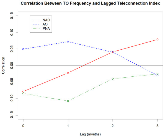
Figure 7.
Monthly TO frequency lag-correlated with our three monthly variability indices (NAO—red; AO—blue; PNA—green). The x-axis corresponds to the lagged period in months prior to the TO frequency month of interest.
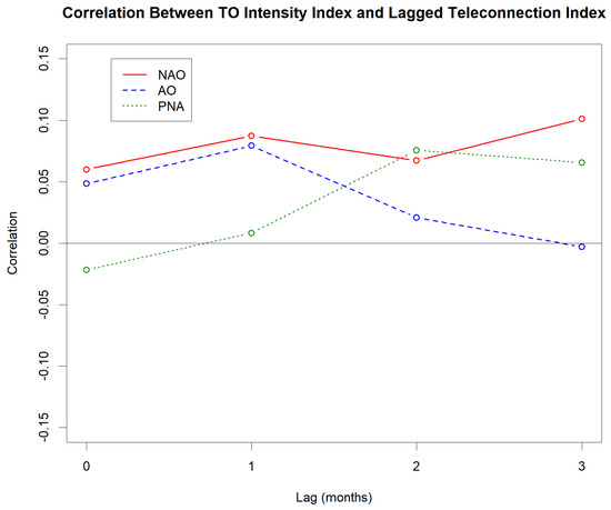
Figure 8.
Same as Figure 7, but for average TO monthly intensity.
The relationship with TO frequency remained fairly weak (similar to ENSO). The strongest lagged correlation with TO frequency (r = −0.107, p = 0.003) was a one-month lag with the PNA (lag-1; Figure 7), which showed statistical significance, owing to the higher monthly frequency being considered. While relatively weak, this relationship suggests that a negative PNA phase is associated with a higher monthly TO frequency, a result that holds for all four lags considered (though it is strongest with lag-1). The AO showed the weakest overall relationships, though the lag-1 AO did have a statistically significant correlation (r = 0.072, p = 0.05), suggesting that a positive AO was supportive of increased TO frequency. The NAO showed an interesting pattern of having an almost identical correlation with a flipped sign at lag-0 and lag-3 (lag-0 correlation of -0.079 [p = 0.032]; lag-3 correlation of 0.079 [p = 0.032]). This result is consistent with the seasonal nature of the NAO [33] and suggests a periodic relationship between the NAO and TO frequency, which may offer seasonal-level TO predictability.
In addition to frequency, we explored the relationship between monthly TO intensity and these monthly variability indices (Figure 8). In general, the results were less robust than those for TO frequency, as the highest correlation of all considered was a 3-month lagged correlation with the NAO at 0.101 (p = 0.006). In this instance, the NAO showed a consistent positive correlation with TO intensity and the overall strongest relationship of all teleconnections. Interestingly, the results again showed a tendency towards fewer but more intense outbreaks associated with a positive PNA. Additionally, the AO showed a declining correlation with increasing lag and was consistently positively correlated with TO intensity (consistent with the TO frequency and the AO discussed above).
As a final analysis, we combined the highest correlated (positive or negative) teleconnection lag for TO frequency and TO average monthly intensity (separately) in a multivariate analysis to establish the net variance explained by all teleconnections. Since these patterns do not work independently but instead co-exist within the geopotential height field, this approach offers insight into the net contribution of all three monthly indices when describing monthly TO frequency or intensity. Table 3 and Table 4 below show the results of an analysis of variance (ANOVA) on these multivariate regressions and reinforce the limited predictability offered by these indices.
Table 3.
Analysis of variance for monthly TO frequency (predictand) versus three teleconnection predictors.
Table 4.
Same as Table 3, but for monthly TO average intensity.
For monthly TO frequency, lag-1 PNA and AO, coupled with lag-0 NAO, offered the highest correlations (−0.107, 0.072, and −0.079, respectively). The ANOVA using these three predictors for TO frequency (Table 3) showed that only a small fraction of total TO frequency variability is explained by these teleconnections (0.8%), suggesting they offer little TO frequency predictability without additional predictors being added.
The monthly TO intensity results offered more interesting (and statistically significant, p = 0.003) multivariate regression results (Table 4). Here, the three top-correlated teleconnections were the lag-3 NAO (r = 0.101), lag-2 PNA (r = 0.076), and the lag-1 AO (r = 0.079). A deeper analysis of the individual regression coefficients showed that both the lag-2 PNA and lag-3 NAO offered statistically significant fits (p = 0.005 and p = 0.030, respectively) to TO intensity, though collectively the three indices still only explained roughly 2% of the total TO intensity variability. In general, the weak nature of these relationships is unsurprising given the chaotic nature of TO occurrence in a given month or year. Additional analyses will be necessary in future work to determine if stronger relationships between these measures of TO frequency and intensity and monthly variability can be established.
4. Discussion and Conclusions
Many limitations exist when quantifying TO variability for climate-related purposes. Seemingly simple aspects such as defining a TO remain elusive and study-dependent, which affects the viability of applying prior TO research to such work. This study addresses that limitation by offering a TO definition that considers tornado occurrence confined to a single tornado day and a discrete spatial region. From this definition, it is possible to derive numerous climatological aspects of TOs, including their annual and monthly variability. As a result, we are able to explore the role of natural interannual and monthly variability in controlling TO activity in the United States. We also found that on average, both TO frequency and intensity are decreasing over time, though these changes were small (roughly 1 outbreak per year fewer every 4–5 years).
In general, the relationships between TO frequency and intensity with the leading mode of interannual variability (ENSO) were weak and not statistically significant. A few patterns were evident in the results, including the slight increase in the number of TOs during El Niño conditions and more annual TO count variability during La Niña conditions. As is well established, El Niño conditions result in an equatorward shift in the polar jet stream, which expectedly brings an increase in extratropical activity in the midlatitudes that could be associated with TOs. However, this equatorward shift also reduces the midlatitude temperature gradient such that while TO frequency may increase, the ingredients for TO strength may be limited owing to increased static stability. During La Niña conditions, the poleward shift of the jet stream creates less predictable and more highly variable TO occurrences, but those TOs that do occur typically have additional thermodynamic energy available and on average produce more intense TOs. These results somewhat contrast with those of [1,2], though their study defined a TO based on tornado days, not discrete tornado regions, and was limited to a winter and early spring study period. Additional studies [34,35] also utilized either different definitions of a TO based on “large numbers of tornadoes” [34] or focused on tornadoes explicitly instead of outbreaks [35]. These inconsistencies in prior studies suggest that methodological considerations are very important when assessing the TO relationship with interannual climate variability. This further reinforces the importance of a consistent TO definition in describing these relationships.
We also explored how monthly climate variability relates to monthly TO occurrence and intensity using a similar approach (but with the NAO, AO, and PNA teleconnections, since ENSO tends to vary on longer timescales). In general, we found that the strongest relationship when describing TO frequency (Figure 7) was a negative correlation with the lag-1 PNA (r = −0.107), suggesting a negative PNA results in a slight (and statistically significant) increase in TO activity. Since a negative PNA results in lower heights in the western U.S., this result is consistent with the expectations of synoptic conditions underlying TOs [10], given that most TOs occur in the central or Mississippi River Valley regions of the United States. The results for the other two teleconnections were less pronounced, though a negative NAO at lag-0 and 1 did show some relationship with the TO frequency (likely from wintertime TOs). The TO intensity results (Figure 8) were less pronounced compared to those for the TO frequency and revealed somewhat opposite reasoning, namely that a positive PNA and NAO resulted in stronger TOs. As a positive PNA/NAO may enhance the thermal gradient comprising the outbreak environment, it was plausible to expect a result similar to that with ENSO: namely, that the positive phase creates more intense TOs when they do occur (though it is not as often).
In general, the results presented herein demonstrate a potential utility of a TO intensity index scheme when quantifying climate-related trends in TOs. The strength of the relationships was notably weak, but as seen in [36], there is seasonality to tornado activity that should be explored further and possibly removed from the tornado data prior to conducting these types of analyses. Such an effort could improve monthly TO predictability. Additionally, the limited study period for annual analyses, as well as the anthropogenic signals within the tornado data themselves, created unique challenges when quantifying TO intensity. Our approach offered one method to work around such challenges, but there are clearly other methods by which this could be achieved that should be explored in future work.
Despite the challenges and limitations of this study, the overall results provide a characterization of TO intensity that can be used when exploring relationships with climate variability. Future work will begin by quantifying the underlying atmospheric conditions associated with different magnitudes of our intensity index to offer additional insight into the large-scale conditions that make TOs stronger. The TO intensity index also allows for a deeper exploration into the spatial trends in TOs (similar to the work in [37]), which will be addressed in subsequent analyses. Additional future work will also explore the utility of this TO intensity index in forecasting TOs for an upcoming tornado season.
Author Contributions
Conceptualization, A.M., K.S., and A.K.; methodology, A.M. and A.K.; software, K.S. and A.K.; validation, A.M., K.S., and A.K.; formal analysis, A.M., K.S., and A.K.; investigation, A.M., K.S., and A.K.; resources, A.M.; data curation, K.S. and A.K.; writing—original draft preparation, A.M.; writing—review and editing, A.M., K.S., and A.K.; visualization, A.M. and K.S.; supervision, A.M.; project administration, A.M. All authors have read and agreed to the published version of the manuscript.
Funding
This research received no external funding.
Data Availability Statement
All data used in this study are publicly available from the National Oceanic and Atmospheric Administration’s Storm Prediction Center (https://www.spc.noaa.gov, accessed 1 June 2024) or from the National Oceanic and Atmospheric Administration’s Climate Prediction Center (https://www.cpc.ncep.noaa.gov, accessed 4 June 2024).
Conflicts of Interest
The authors declare no conflicts of interest.
References
- Cook, A.R.; Leslie, L.M.; Parsons, D.B.; Schaefer, J.T. The impact of El Niño-Southern Oscillation (ENSO) on winter and early spring U.S. tornado outbreaks. J. Appl. Meteor. Climo. 2017, 56, 2455–2478. [Google Scholar] [CrossRef]
- Cook, A.R.; Schaefer, J.T. The relation of El Niño-Southern Oscillation (ENSO) to winter tornado outbreaks. Mon. Wea. Rev. 2008, 136, 3121–3137. [Google Scholar] [CrossRef]
- Sparrow, K.R.; Mercer, A.E. Predictability of US tornado outbreak seasons using ENSO and northern hemisphere geopotential height variability. Geosmin. Front. 2016, 7, 21–31. [Google Scholar] [CrossRef]
- Carr, J.A. A preliminary report on the tornadoes of 21–22 March 1952. Mon. Wea. Rev. 1952, 80, 50–58. [Google Scholar] [CrossRef]
- Beebe, R.G. Tornado composite charts. Mon. Wea. Rev. 1956, 84, 127–142. [Google Scholar] [CrossRef]
- Wolford, L.V. Tornado Occurrences in the United States; U.S. Government Printing Office: Washington, DC, USA, 1960; pp. 339–343. [Google Scholar]
- Maddox, R.A.; Gray, W.M. A study of tornado proximity data and an observationally derived model of tornado genesis. Colo. State Univ. Atmos. Sci. Pap. 1973, 212, 202. [Google Scholar]
- Galway, J.G. Some climatological aspects of tornado outbreaks. Mon. Wea. Rev. 1977, 105, 477–484. [Google Scholar] [CrossRef]
- Pautz, M.E. Severe Local Storm Occurrences, 1955–1967; Environmental Science Services Administration Rep.: Rockville, MD, USA, 1969; p. 71. [Google Scholar]
- Mercer, A.E.; Shafer, C.M.; Doswell, C.A.; Leslie, L.M.; Richman, M.B. Synoptic composites of tornadic and nontornadic outbreaks. Mon. Wea. Rev. 2012, 140, 2590–2608. [Google Scholar] [CrossRef]
- Doswell, C.M.; Edwards, R.; Thompson, R.L.; Hart, J.A.; Crosbie, K.C. A simple and flexible method for ranking severe weather events. Wea. Forecast. 2006, 21, 939–951. [Google Scholar] [CrossRef]
- Ćwik, P.; McPherson, R.A.; Brooks, H.E. What is a tornado outbreak?: Perspectives through time. Bull. Amer. Meteor. Soc. 2021, 102, E817–E835. [Google Scholar] [CrossRef]
- American Meteorological Society Glossary of Meteorology. Available online: https://glossary.ametsoc.org/wiki/Tornado_outbreak (accessed on 5 June 2024).
- Shafer, C.M.; Doswell, C.A. A multivariate index for ranking and classifying severe weather outbreaks. Elec. J. Sev. Storms Meteor. 2010, 5, 1–39. [Google Scholar] [CrossRef]
- Shafer, C.M.; Doswell, C.A. Using kernel density estimation to identify, rank, and classify severe weather outbreak events. Elec. J. Sev. Storms Meteor. 2011, 6, 1–28. [Google Scholar] [CrossRef]
- Schaefer, J.T.; Edwards, R. 1999: The SPC tornado/severe thunderstorm database. Preprints, 11th Conf. Applied Climo. 1999. Available online: https://www.spc.noaa.gov/publications/schaefer/database.htm (accessed on 1 June 2024).
- Fuhrmann, C.M.; Konrad, C.E.; Kovach, M.M.; McLeod, J.T.; Schmitz, W.G.; Dixon, P.G. Ranking of tornado outbreaks across the United States and their climatological impacts. Wea. Forecast. 2014, 29, 684–701. [Google Scholar] [CrossRef]
- Edwards, R.; Brooks, H.E.; Cohn, H. Changes in tornado climatology accompanying the enhanced Fujita scale. J. Appl. Meteor. Climo. 2021, 60, 1465–1482. [Google Scholar] [CrossRef]
- Barnston, A.G.; Chelliah, M.; Goldenberg, S.B. Documentation of a highly ENSO-related SST region in the equatorial Pacific, research note. Atmos-Ocean 1997, 35, 367–383. [Google Scholar] [CrossRef]
- Huang, B.; Thorne, P.W.; Banzon, V.F.; Boyer, T.; Chepurin, G.; Lawrimore, J.H.; Menne, M.J.; Smith, T.M.; Vose, R.S.; Zhang, H.-M. Extended reconstructed sea surface temperature version 5 (ERSSTv5): Upgrades, validations, and intercomparisons. J. Clim. 2017, 30, 8179–8205. [Google Scholar] [CrossRef]
- Barnston, A.B.; Livezey, R. Classification, seasonality, and persistence of low-frequency atmospheric circulation patterns. Mon. Wea. Rev. 1987, 115, 1083–1126. [Google Scholar] [CrossRef]
- Thompson, D.; Wallace, J. The arctic oscillation signature in wintertime geopotential heights and temperature fields. Geophys. Res. Lett. 1998, 25, 1297–1300. [Google Scholar] [CrossRef]
- Climate Prediction Center. Teleconnection Indices. Available online: https://www.cpc.ncep.noaa.gov (accessed on 4 June 2024).
- SPC National Severe Weather Database Browser Severe Plot. Available online: https://www.spc.noaa.gov/climo/online/sp3/ (accessed on 5 June 2024).
- Doswell, C.A.; Brooks, H.E.; Kay, M.P. Climatological estimates of daily nontornadic severe thunderstorm probability for the United States. Wea. Forecast. 2005, 20, 577–595. [Google Scholar] [CrossRef]
- Cristianini, N.; Shawe-Taylor, J. An Introduction to Support Vector Machines and Other Kernel-Based Methods; Cambridge University Press: Cambridge, UK, 2000; pp. 149–161. [Google Scholar]
- Fujita, T. Jumbo tornado outbreak of 3 April 1974. Weatherwise 1974, 27, 116–126. [Google Scholar] [CrossRef]
- Corfidi, S.; Weiss, S.; Kain, J.; Corfidi, S.; Rabin, R.; Levit, J. Revisiting the 3-4 April 1974 super outbreak of tornadoes. Wea. Forecast. 2010, 25, 465–510. [Google Scholar] [CrossRef]
- Knupp, K.; Murphy, T.; Coleman, T.; Wade, R.; Mullins, S.; Schultz, C.; Schultz, E.; Carey, L.; Sherrer, A.; McCaul, E.; et al. Meteorological overview of the devastating 27 April 2011 tornado outbreak. Bull. Am. Meteor. Soc. 2014, 95, 1041–1062. [Google Scholar] [CrossRef]
- Chasteen, M.; Koch, S. Multiscale aspects of the 26-27 April 2011 tornado outbreak. Part I: Outbreak chronology and environmental evolution. Mon. Wea. Rev. 2022, 150, 309–335. [Google Scholar] [CrossRef]
- Fujita, T.; Bradbury, D.; Thullenar, C. Palm Sunday tornadoes of 11 April 1965. Mon. Wea. Rev. 1970, 98, 29–69. [Google Scholar] [CrossRef]
- Efron, B.; Tibshirani, R. An Introduction to the Bootstrap; CRC Press: Boca Raton, FL, USA, 1994; p. 456. [Google Scholar]
- Wang, L.; Ting, M.; Kushner, P. A robust empirical seasonal prediction of winter NAO and surface climate. Sci. Rep. 2017, 7, 279. [Google Scholar] [CrossRef] [PubMed]
- Bove, M. Impacts of ENSO on United States tornado activity. Prepr. 19th Conf. Sev. Local Storms 1998, 313, 316. [Google Scholar]
- Allen, J.; Molina, M.; Gensini, V. Modulation of annual cycle of tornadoes by El Niño-Southern Oscillation. Geophys. Res. Lett. 2018, 45, 5708–5717. [Google Scholar] [CrossRef]
- Brooks, H.; Doswell, C.; Kay, M. Climatological estimates of local daily tornado probability for the United States. Wea. Forecast. 2003, 18, 626–640. [Google Scholar] [CrossRef]
- McCormick, A.; Mercer, A. Diagnosing the relationship between the Madden–Julian Oscillation and United States severe convective weather outbreaks. Int. J. Climatol. 2023, 43, 6963–6978. [Google Scholar] [CrossRef]


Disclaimer/Publisher’s Note: The statements, opinions and data contained in all publications are solely those of the individual author(s) and contributor(s) and not of MDPI and/or the editor(s). MDPI and/or the editor(s) disclaim responsibility for any injury to people or property resulting from any ideas, methods, instructions or products referred to in the content. |
© 2024 by the authors. Licensee MDPI, Basel, Switzerland. This article is an open access article distributed under the terms and conditions of the Creative Commons Attribution (CC BY) license (https://creativecommons.org/licenses/by/4.0/).