
Urban Climate Dynamics: Analyzing the Impact of Green Cover and Air Pollution on Land Surface Temperature—A Comparative Study Across Chicago, San Francisco, and Phoenix, USA


Abstract
1. Introduction
2. Materials
2.1. Study Area
2.2. Data
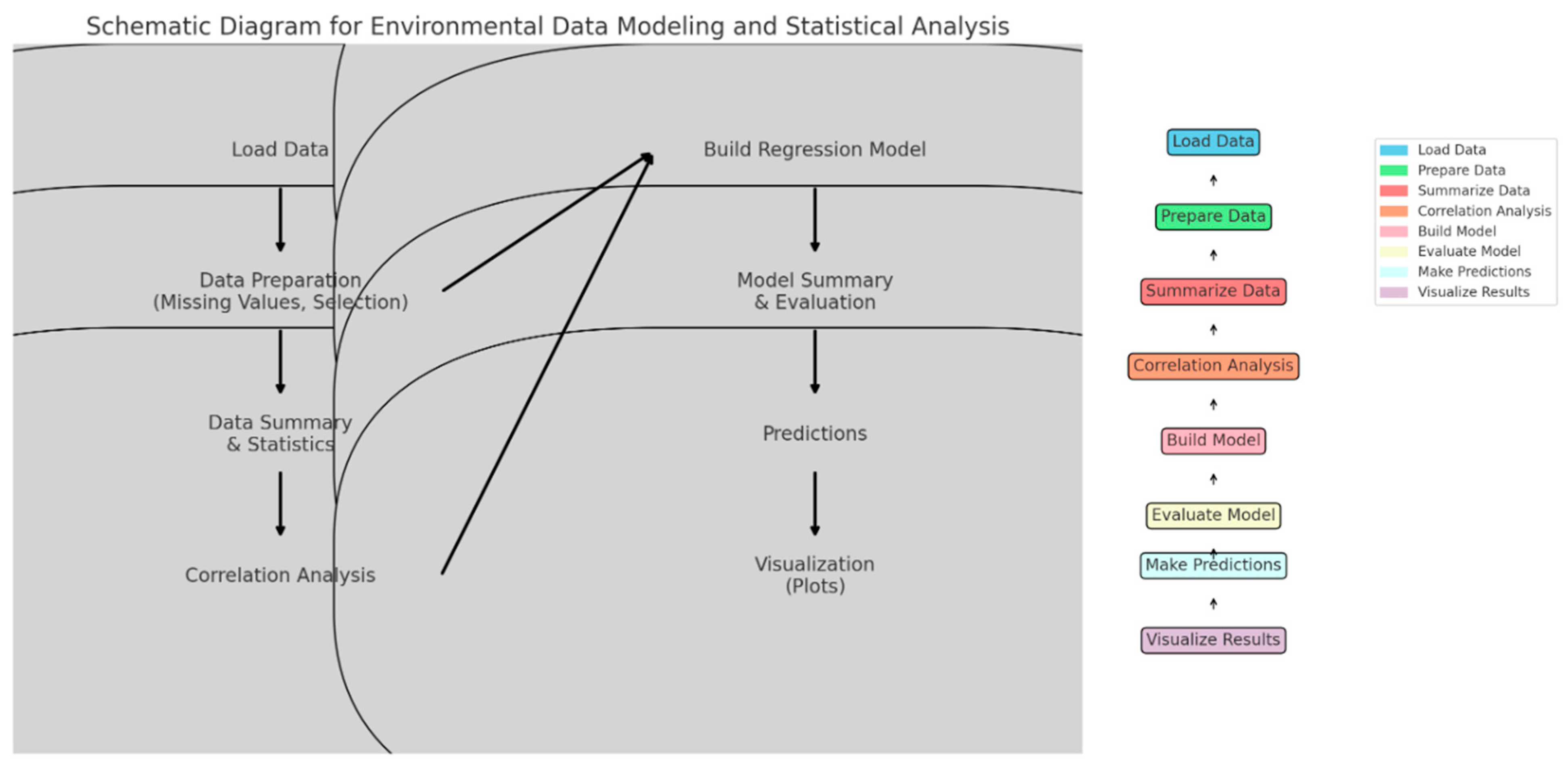
3. Method
3.1. Multivariate Linear Regression Analysis
- is the dependent variable LST (urban heat island effect);
- are the independent variables (SO2, NO2, CO, O3, and NDVI);
- is the intercept (constant term);
- are the coefficients (regression coefficients) representing the effect of each independent variable on the dependent variable;
- is the error term (residuals), representing the difference between the observed and predicted values of the dependent variable.
- n is the number of observations;
- is the observed value of the dependent variable for observation ;
- is the predicted value of the dependent variable for observation i based on the regression model.
3.2. Correlation Analysis
- is the correlation coefficient between variables and ;
- and are individual observations of variables and , respectively;
- and are the means of variables and , respectively;
- is the number of observations.
- is the correlation coefficient between the th and th variables.
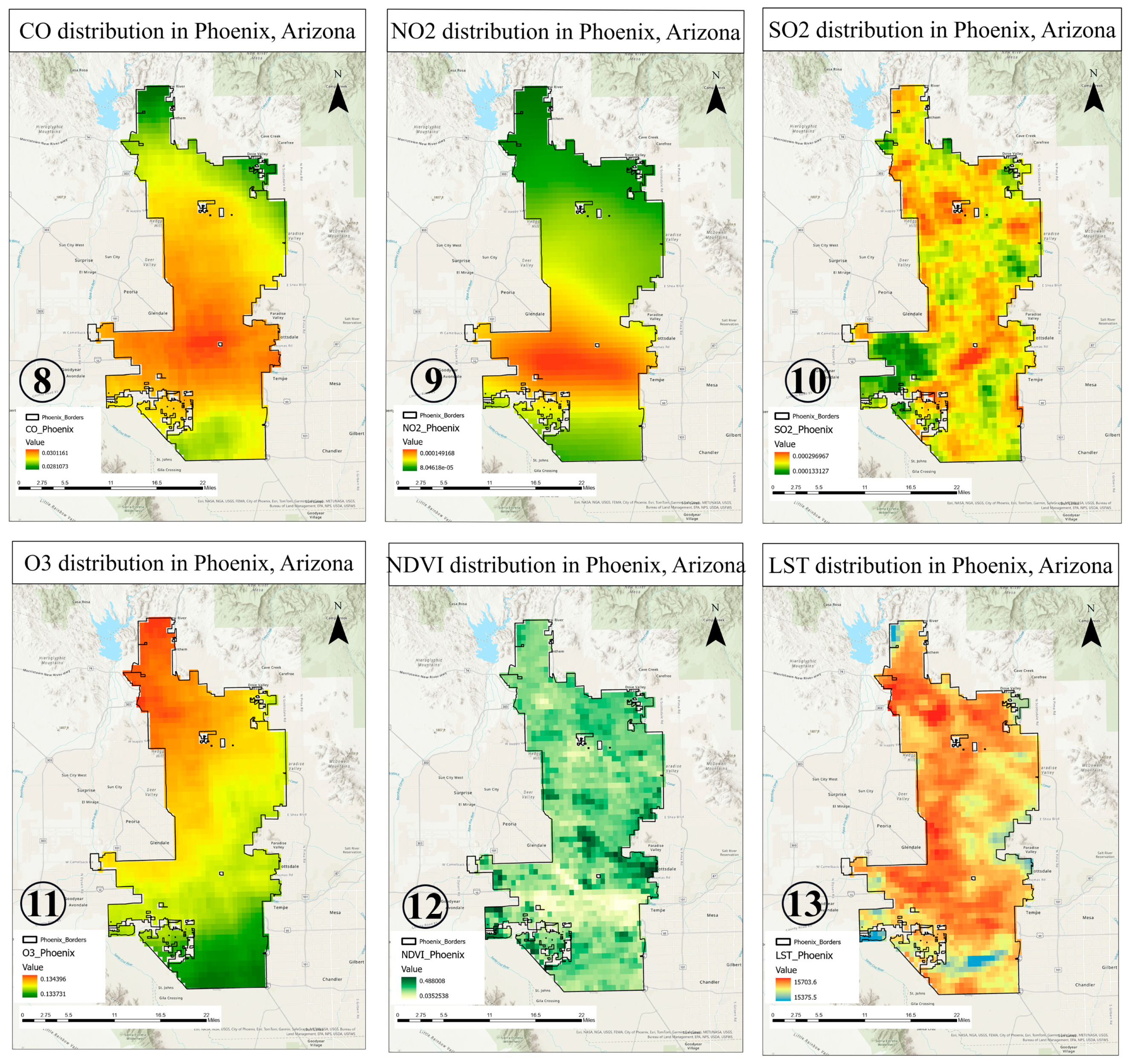
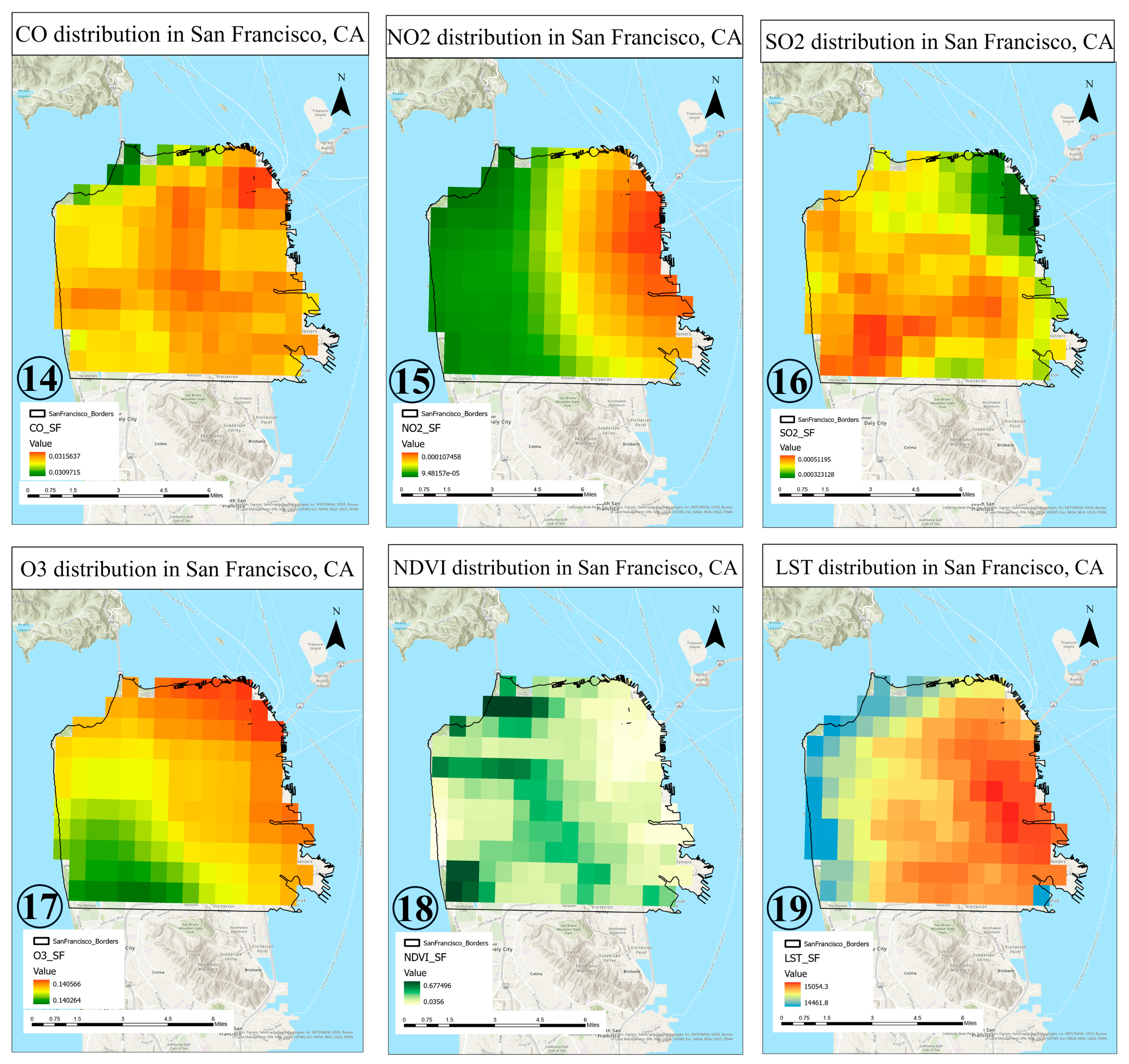
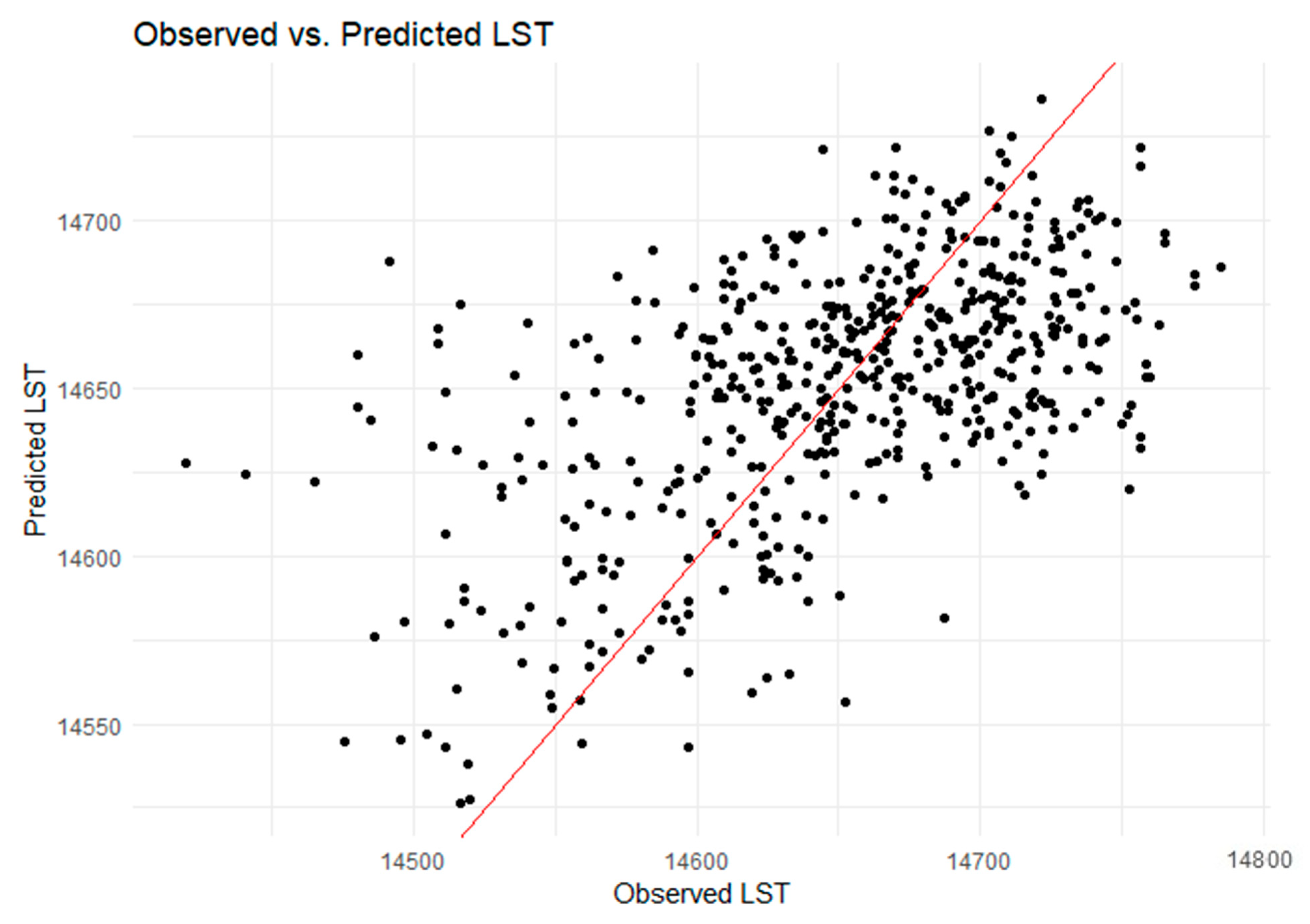
4. Results
5. Discussion
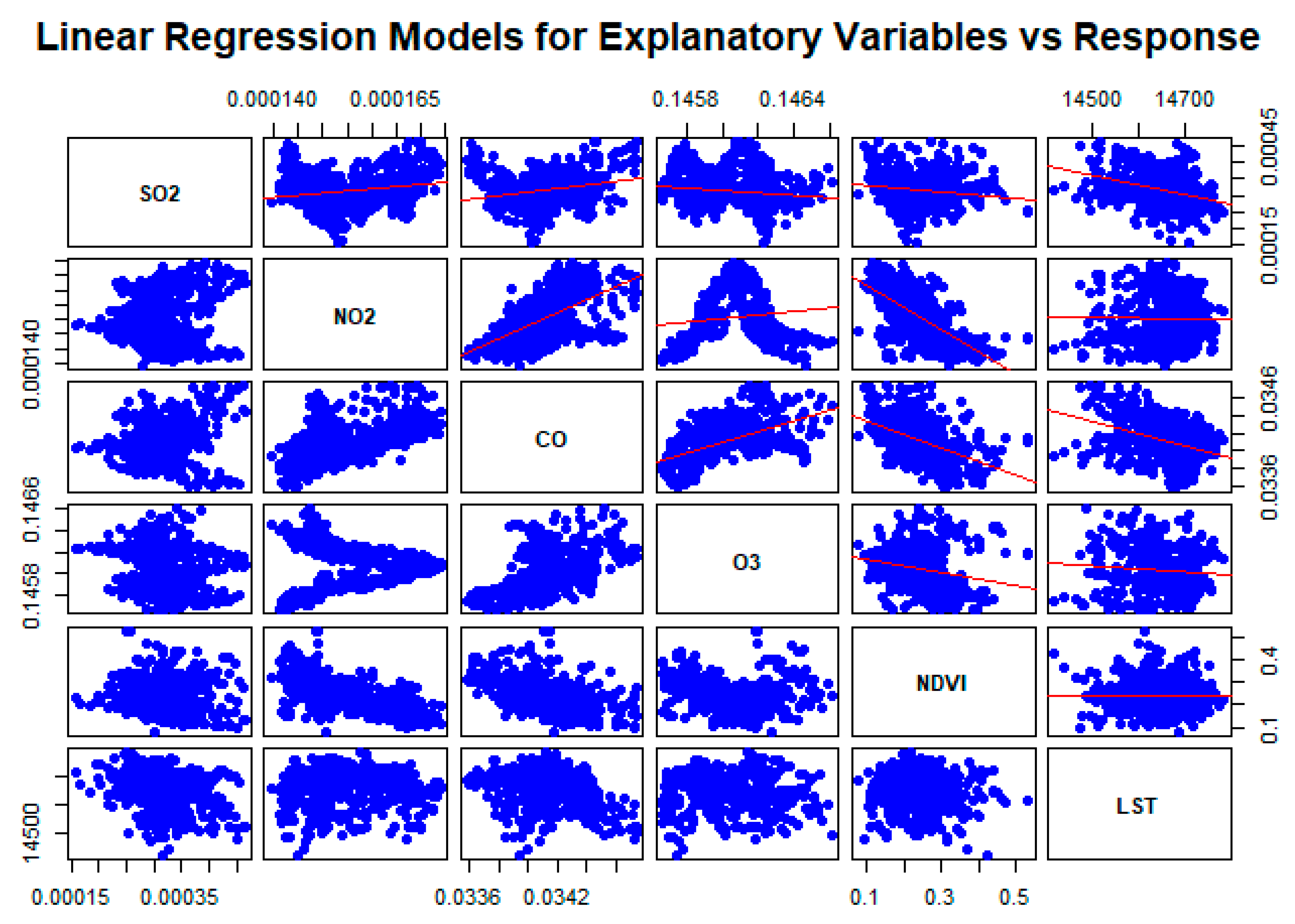
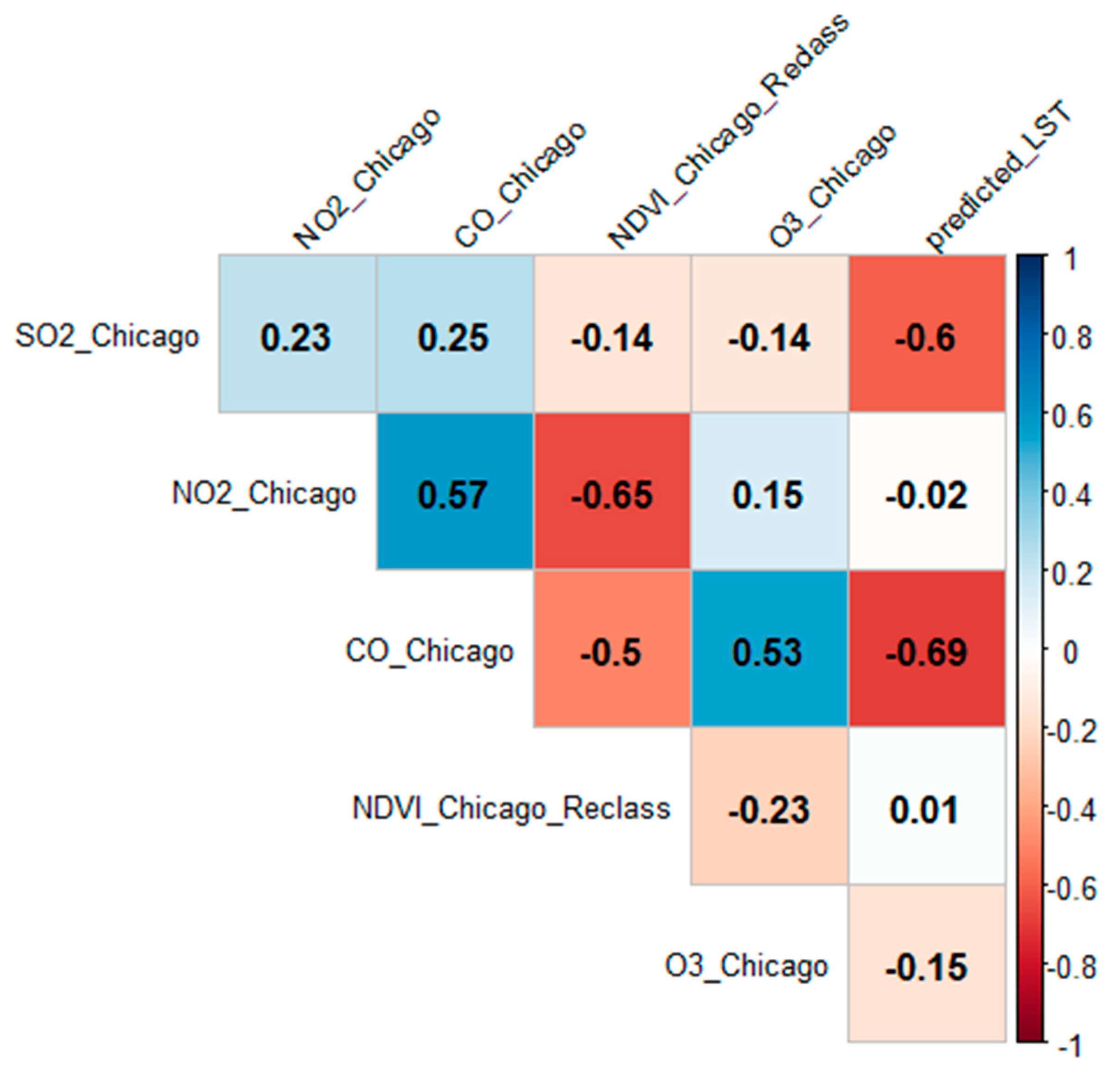
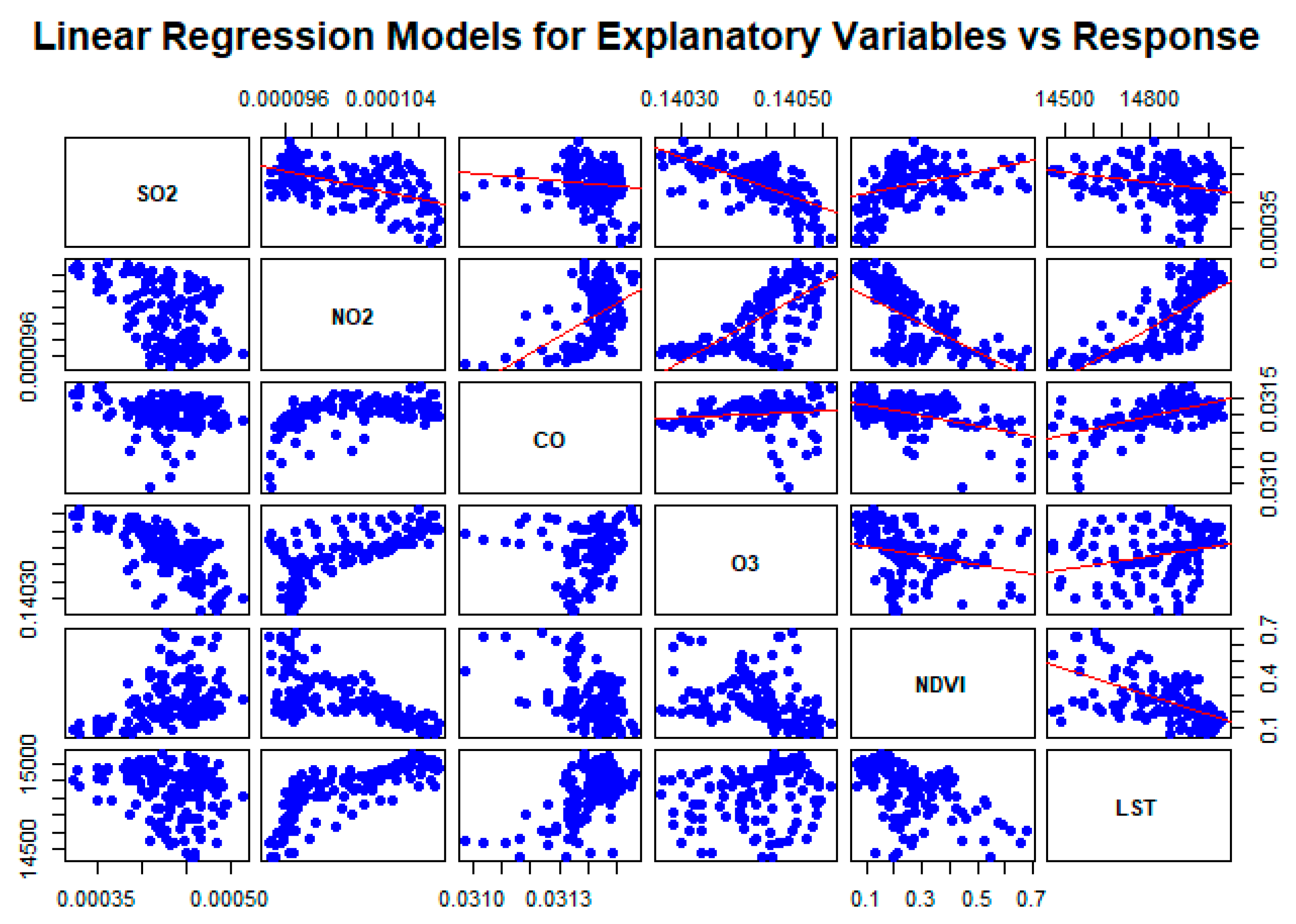
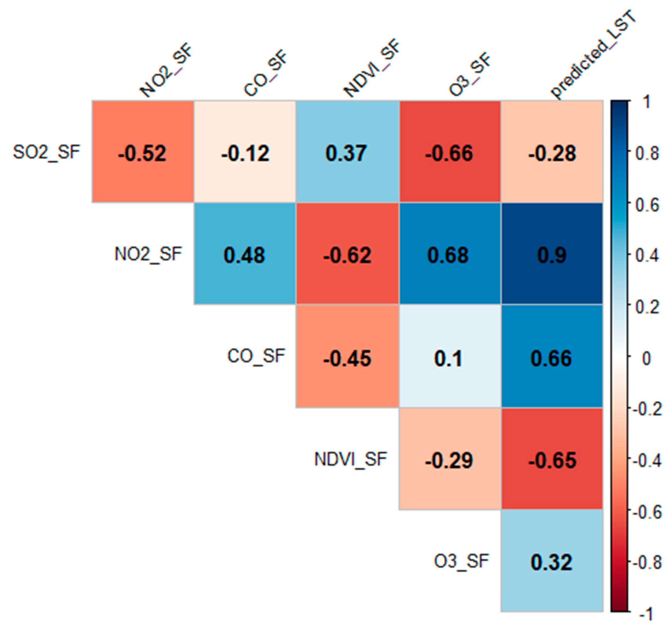
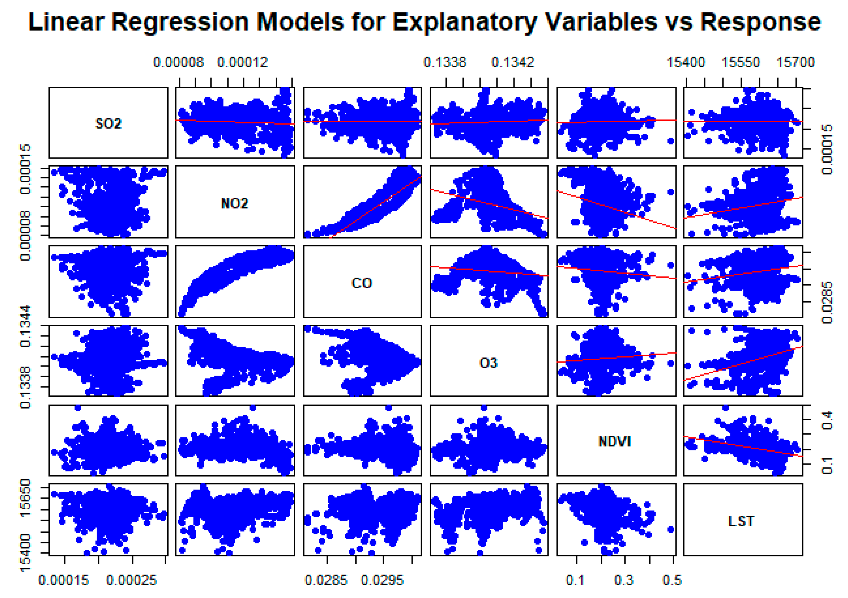
| Positive Slope in Chicago, San Francisco, and Phoenix: | The positive slope observed in these cities suggests a systematic relationship where changes in one variable are associated with changes in another. For example, increased NO2 and CO levels might be related to higher LST, which could be due to the urban heat island effect exacerbated by pollution and lack of vegetation. |
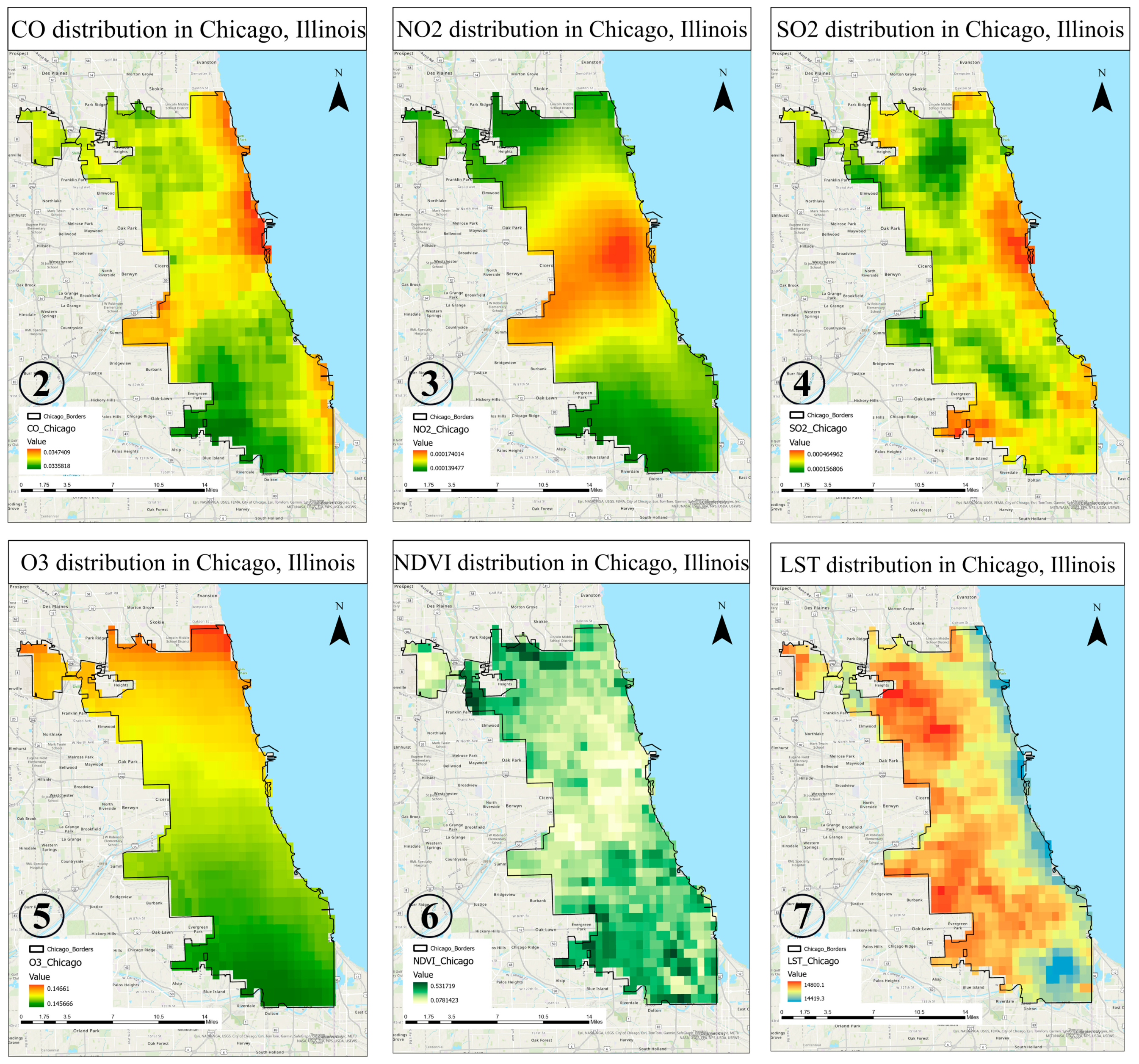
| Normalized Difference Vegetation Index (NDVI): | NDVI is crucial in this analysis as it represents vegetation density and health. Higher NDVI values typically indicate more vegetation, which can lead to lower LST due to the cooling effects of plants. Conversely, lower NDVI values, indicating less vegetation, can correlate with higher LST and increased pollution levels. |
| Land Surface Temperature (LST): | LST provides a direct measure of the urban heat island effect. The relationship between LST and air pollutants is significant, as pollutants can trap heat, leading to higher surface temperatures. |
| Air Pollutants (SO2, NO2, CO, O3): | These pollutants are not only health hazards, but also contribute to atmospheric warming. Their relationship with NDVI and LST can indicate how urbanization and pollution control measures impact urban climates. |
| Geographical and Climatic Differences | Climate Variability: Different cities have distinct climates. For instance, Phoenix has a desert climate, Chicago has a temperate climate, and San Francisco has a Mediterranean climate. These climatic differences affect how pollutants interact with vegetation and land surface temperatures. Geographical Features: The topography and proximity to natural features (e.g., oceans, mountains) can impact pollution dispersion and temperature regulation. San Francisco’s coastal location, for instance, leads to different atmospheric dynamics compared to landlocked Phoenix and Chicago. |
| Urban Infrastructure and Land Use | Urban Density: Variations in urban density can influence pollution levels and heat absorption. Highly urbanized areas with dense infrastructure may exhibit stronger urban heat island effects, affecting LST. Land Use Patterns: Differences in land use, such as the extent of green spaces, industrial areas, and residential zones, can lead to variations in NDVI and its relationship with LST and pollutants. |
| Vegetation Types and Coverage | Vegetation Types: Different types of vegetation (e.g., deciduous forests in Chicago, desert vegetation in Phoenix) respond differently to pollution and heat. This can lead to varying NDVI values and their correlation with LST and pollutants. Seasonal Variations: Seasonal changes affect vegetation health and density, which in turn influence NDVI and its interaction with LST and air pollutants. |
| Socio-Economic and Policy Factors | Industrial Activities: The levels and types of industrial activities differ between cities, affecting the emission of pollutants. For example, a city with heavy industry may have higher levels of SO2 and NO2 compared to a predominantly residential city. Pollution Control Measures: Different cities may have varying levels of pollution control regulations and practices. Stricter regulations in one city could lead to lower pollutant levels, affecting the observed correlations. Urban Planning Policies: Policies related to green space development, transportation, and energy usage can significantly impact NDVI and LST. |
6. Conclusions
Author Contributions
Funding
Institutional Review Board Statement
Informed Consent Statement
Data Availability Statement
Conflicts of Interest
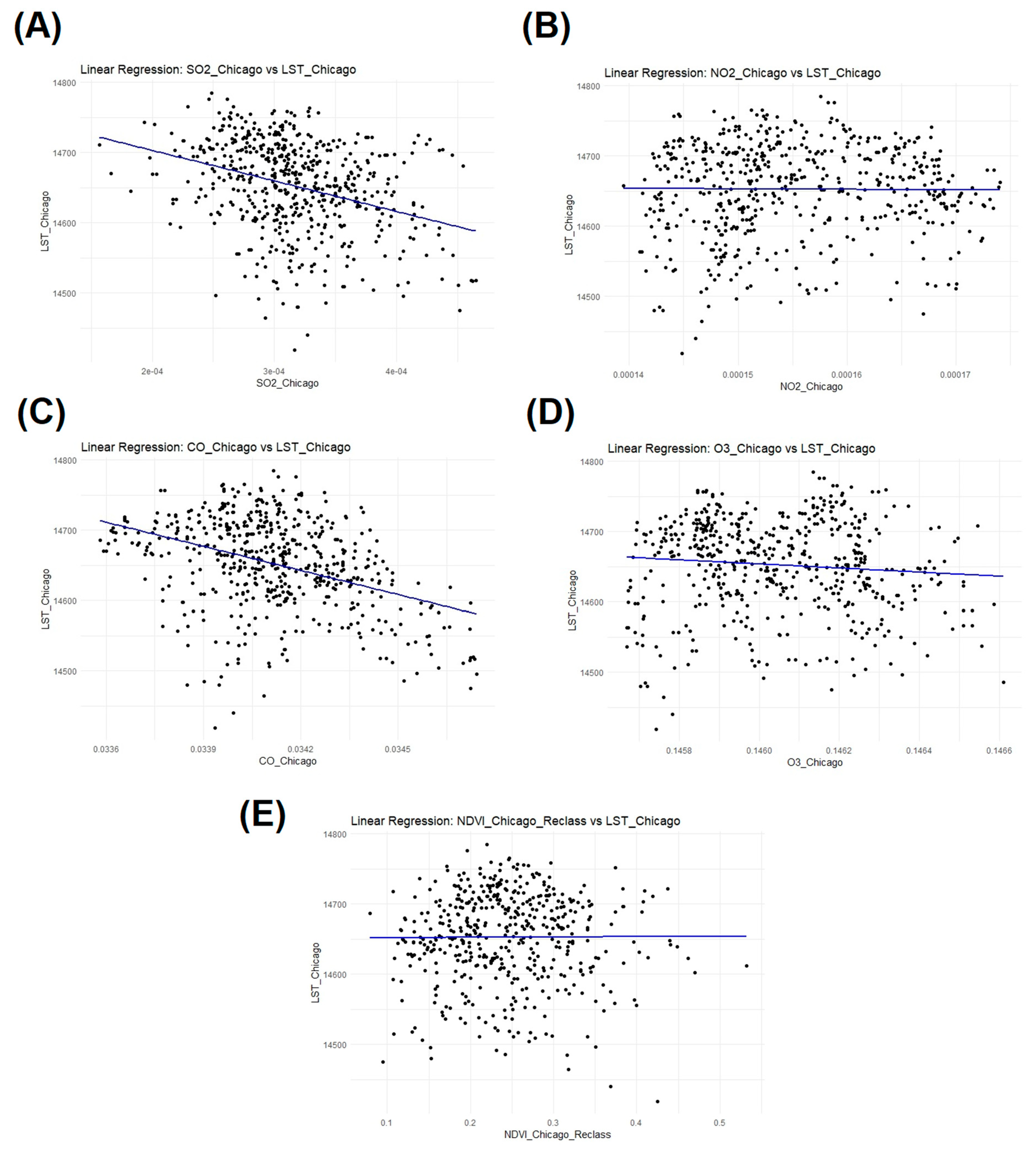
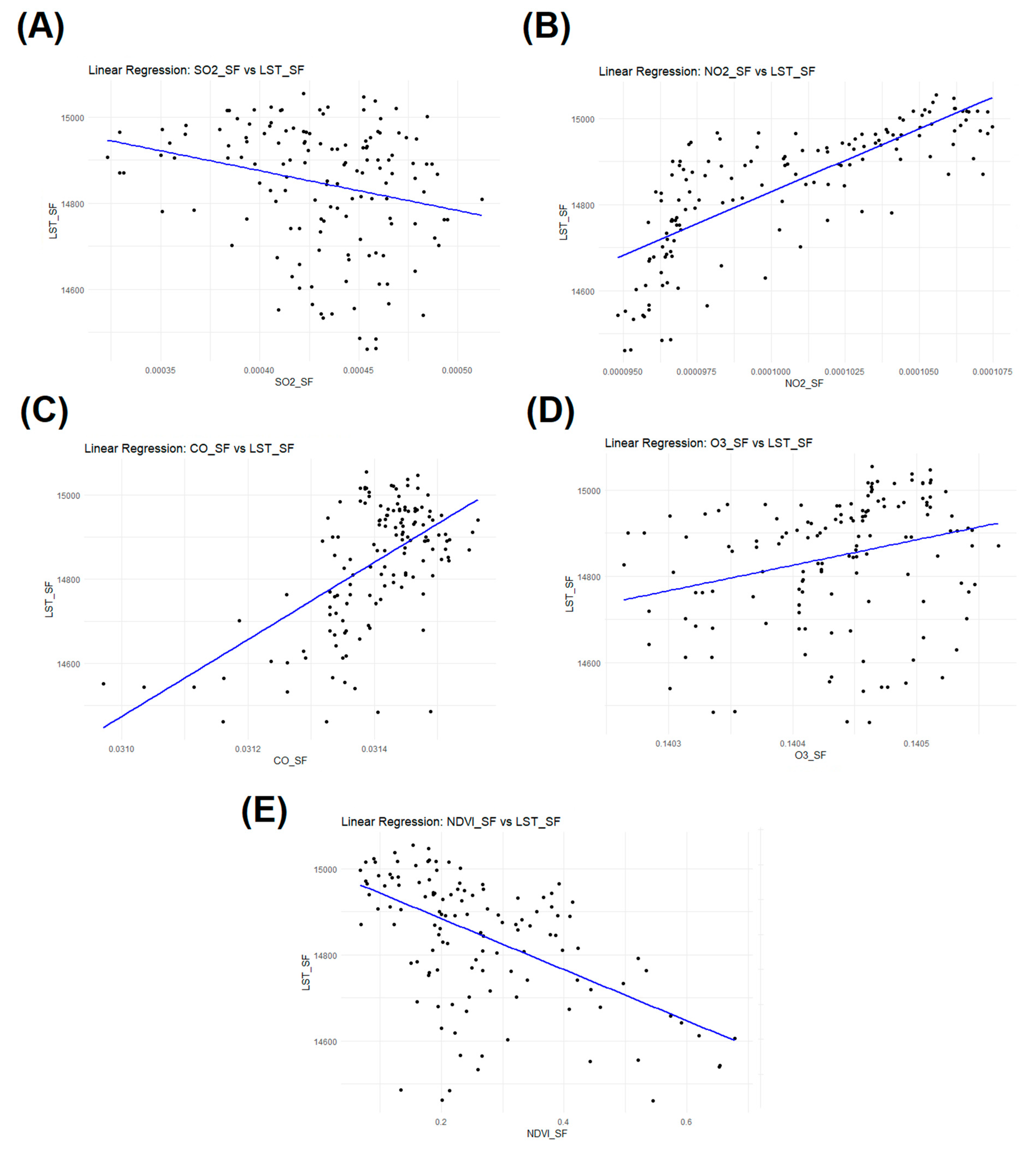
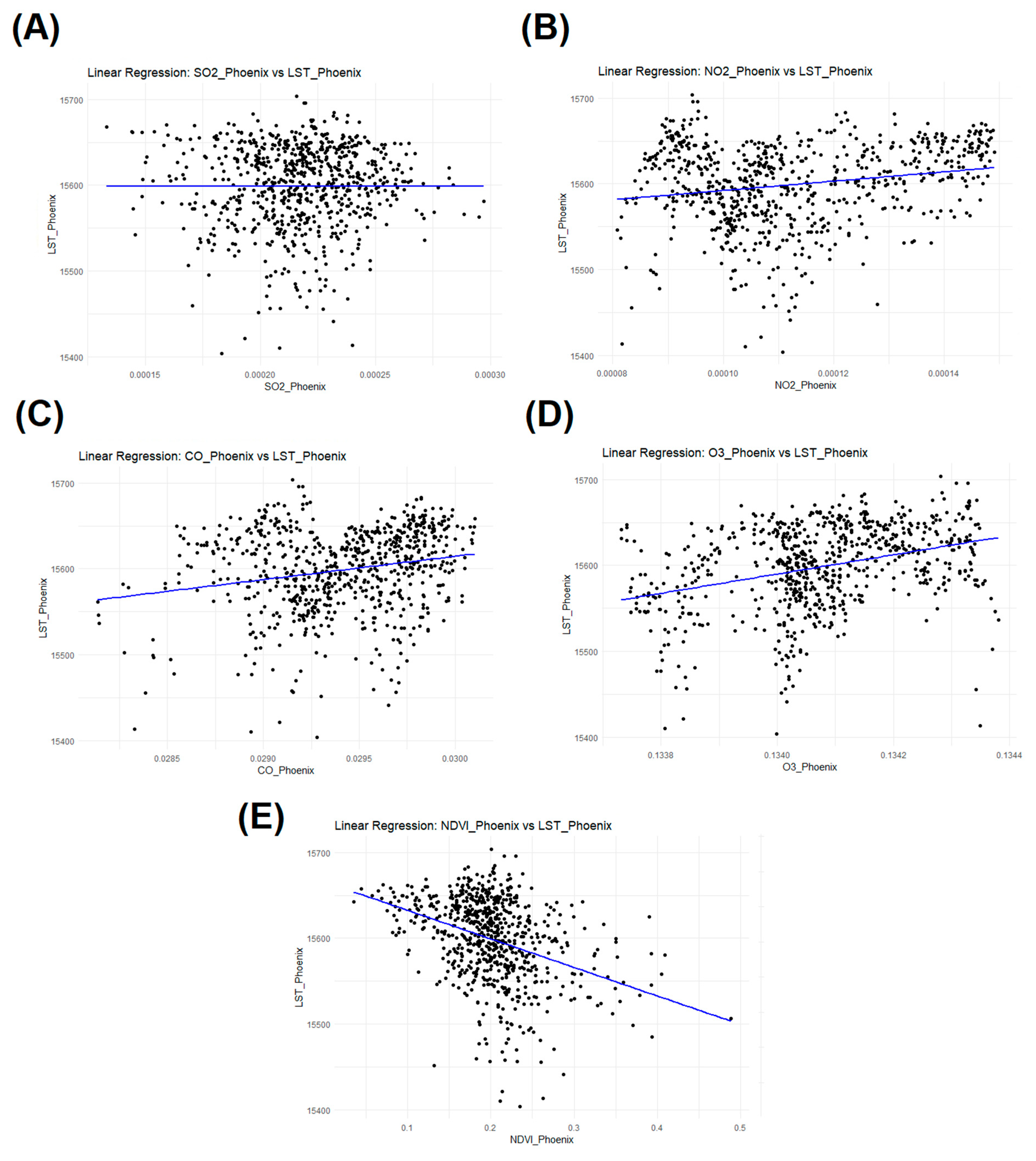
Appendix A. Simple Linear Regression Results

| Coefficients: | Standard Errors | R-Squared | p-Value |
|---|---|---|---|
| (Intercept) | 11.96263 | 0 | |
| SO2_Chicago | 37,275.79 | 0.1239386 | 1.894694 × 10⁻²⁹ |
| (Intercept) | 37.28437 | 0 | |
| NO2_Chicago | 239,376.3 | 8.883425 × 10⁻⁵ | 0.7703177 |
| (Intercept) | 283.6162 | 0 | |
| CO_Chicago | 8313.406 | 0.1642344 | 2.519089 × 10−39 |
| (Intercept) | 1503.19 | 1.204059 × 10⁻³³ | |
| O3_Chicago | 10,292.99 | 0.00821565 | 0.004901358 |
| (Intercept) | 7.029288 | 0 | |
| NDVI_Chicago_Reclass | 27.72584 | 3.546721 × 10⁻⁵ | 0.85364 |
| Coefficients: | Standard Errors | R-Squared | p-Value |
|---|---|---|---|
| (Intercept) | 54.21478 | 0 | |
| SO2_San FranCIsco | 124,699.8 | 0.05686028 | 2.695234 × 10⁻¹³ |
| (Intercept) | 77.98104 | 0 | |
| NO2_San FranCIsco | 775,134.3 | 0.6104262 | 4.292184 × 10−189 |
| (Intercept) | 1349.309 | 2.130909 × 10⁻²³ | |
| CO_San FranCIsco | 42,963.39 | 0.3308995 | 9.944687 × 10−82 |
| (Intercept) | 1349.309 | 2.130909 × 10⁻²³ | |
| CO_San FranCIsco | 42,963.39 | 0.3308995 | 9.944687 × 10−82 |
| (Intercept) | 9548.527 | 1.987411 × 10⁻¹² | |
| O3_San FranCIsco | 67,993.3 | 0.07636868 | 1.677641 × 10⁻¹⁷ |
| (Intercept) | 8.564489 | 0 | |
| NDVI_San FranCIsco | 28.50301 | 0.3211276 | 7.560097 × 10−79 |
| Coefficients: | Standard Errors | R-Squared | p-Value |
|---|---|---|---|
| (Intercept) | 13.55378 | 0 | |
| SO2_Phoenix | 62,064.17 | 3.793562 × 10⁻¹⁰ | 0.9995169 |
| (Intercept) | 10.01575 | 0 | |
| NO2_Phoenix | 88,388.17 | 0.03759978 | 1.156671 × 10⁻⁹ |
| (Intercept) | 119.2396 | 0 | |
| CO_Phoenix | 4053.115 | 0.04457391 | 3.1677 × 10⁻¹¹ |
| (Intercept) | 1340.272 | 0.6729829 | |
| O3_Phoenix | 9996.181 | 0.1151196 | 1.562659 × 10⁻²⁷ |
| (Intercept) | 5.600326 | 0 | |
| NDVI_Phoenix | 26.78363 | 0.1372672 | 6.819469 × 10⁻³³ |
References
- Frosini, G.; Amato, A.; Mugnai, F.; Cinelli, F. The impact of trees on the UHI effect and urban environment quality: A case study of a district in Pisa, Italy. Atmosphere 2024, 15, 123. [Google Scholar] [CrossRef]
- Moreno, R.; Zamora, R.; Moreno-García, N.; Galán, C. Effects of composition and structure variables of urban trees in the reduction of heat islands; case study, Temuco city, Chile. Build. Environ. 2023, 245, 110859. [Google Scholar] [CrossRef]
- Stone, B. The City and the Coming Climate: Climate Change in the Places We Live; Cambridge University Press: Cambridge, UK, 2012. [Google Scholar]
- Bowler, D.E.; Buyung-Ali, L.; Knight, T.M.; Pullin, A.S. Urban greening to cool towns and cities: A systematic review of the empirical evidence. Landsc. Urban Plan. 2010, 97, 147–155. [Google Scholar] [CrossRef]
- Azizi, S.; Azizi, T. The Fractal Nature of Drought: Power Laws and Fractal Complexity of Arizona Drought. Eur. J. Math. Anal. 2022, 2, 17. [Google Scholar] [CrossRef]
- Zhao, L.; Lee, X.; Smith, R.B.; Oleson, K. Strong contributions of local background climate to urban heat islands. Nature 2014, 511, 216–219. [Google Scholar] [CrossRef] [PubMed]
- Rani, M.; Kumar, P.; Pandey, P.C.; Srivastava, P.K.; Chaudhary, B.S.; Tomar, V.; Mandal, V.P. Multi-temporal NDVI and surface temperature analysis for Urban Heat Island inbuilt surrounding of sub-humid region: A case study of two geographical regions. Remote Sens. Appl. Soc. Environ. 2018, 10, 163–172. [Google Scholar] [CrossRef]
- Venkatraman, S.; Kandasamy, V.; Rajalakshmi, J.; Sabarunisha Begum, S.; Sujatha, M. Assessment of urban heat island using remote sensing and geospatial application: A case study in Sao Paulo city, Brazil, South America. J. South Am. Earth Sci. 2024, 134, 104763. [Google Scholar] [CrossRef]
- Sharmin, T.; Chappell, A.; Lannon, S. Spatio-temporal analysis of LST, NDVI and SUHI in a coastal temperate city using local climate zone. Energy Built Environ. 2024, in press. [Google Scholar] [CrossRef]
- Jacobson, M.Z. Atmospheric Pollution: History, Science, and Regulation; Cambridge University Press: Cambridge, UK, 2002. [Google Scholar]
- Seinfeld, J.H.; Pandis, S.N. Atmospheric Chemistry and Physics: From Air Pollution to Climate Change; John Wiley & Sons: Hoboken, NJ, USA, 2006. [Google Scholar]
- Cichowicz, R.; Bochenek, A.D. Assessing the effects of urban heat islands and air pollution on human quality of life. Anthropocene 2024, 46, 100433. [Google Scholar] [CrossRef]
- Han, L.; Zhang, R.; Wang, J.; Cao, S.-J. Spatial synergistic effect of urban green space ecosystem on air pollution and heat island effect. Urban Clim. 2024, 55, 101940. [Google Scholar] [CrossRef]
- Iungman, T.; Khomenko, S.; Barboza, E.P.; Cirach, M.; Gonçalves, K.; Petrone, P.; Erbertseder, T.; Taubenböck, H.; Chakraborty, T.; Nieuwenhuijsen, M. The impact of urban configuration types on urban heat islands, air pollution, CO2 emissions, and mortality in Europe: A data science approach. Lancet Planet. Health 2024, 8, e489–e505. [Google Scholar] [CrossRef] [PubMed]
- Chicago Climate Action Plan. City of Chicago: Chicago, IL, USA. 2022. Available online: https://www.chicago.gov/city/en/sites/climate-action-plan/home.html (accessed on 10 April 2024).
- Hong, T.; Xu, Y.; Sun, K.; Zhang, W.; Luo, X.; Hooper, B. Urban microclimate and its impact on building performance: A case study of San Francisco. Urban Clim. 2021, 38, 100871. [Google Scholar] [CrossRef]
- Chow, W.T.L.; Brennan, D.; Brazel, A.J. Urban heat island research in Phoenix, Arizona: Theoretical contributions and policy applications. Bull. Am. Meteorol. Soc. 2012, 93, 517–530. [Google Scholar] [CrossRef]
- Ighalo, J.O.; Adeniyi, A.G.; Marques, G. Internet of Things for Water Quality Monitoring and Assessment: A Comprehensive Review. In Artificial Intelligence for Sustainable Development: Theory, Practice and Future Applications; Springer: Cham, Switzerland, 2020; pp. 245–259. [Google Scholar]
- Muniz, D.H.F.; Oliveira-Filho, E.C. Multivariate Statistical Analysis for Water Quality Assessment: A Review of Research Published between 2001 and 2020. Hydrology 2023, 10, 196. [Google Scholar] [CrossRef]
- Cheng, X.; He, L.; Lu, H.; Chen, Y.; Ren, L. Optimal Water Resources Management and System Benefit for the Marcellus Shale-Gas Reservoir in Pennsylvania and West Virginia. J. Hydrol. 2020, 540, 412–422. [Google Scholar] [CrossRef]
- He, L.; Shao, F.; Ren, L. Sustainability Appraisal of Desired Contaminated Groundwater Remediation Strategies: An Information-Entropy-Based Stochastic Multi-Criteria Preference Model. Environ. Dev. Sustain. 2020, 23, 1759–1779. [Google Scholar] [CrossRef]
- Gupta, S.; Aga, D.; Pruden, A.; Zhang, L.; Vikesland, P. Data analytics for environmental science and engineering research. Environ. Sci. Technol. 2021, 55, 10895–10907. [Google Scholar] [CrossRef] [PubMed]
- Banerjee, B.; Kundu, S.; Kanchan, R.; Mohanta, A. Examining the relationship between atmospheric pollutants and meteorological factors in Asansol city, West Bengal, India, using statistical modelling. Environ. Sci. Pollut. Res. 2024. online ahead of print. [Google Scholar] [CrossRef] [PubMed]
- Daoud, J.I. Multicollinearity and regression analysis. J. Phys. Conf. Ser. 2017, 949, 012009. [Google Scholar] [CrossRef]
- Marcoulides, K.M.; Raykov, T. Evaluation of variance inflation factors in regression models using latent variable modeling methods. Educ. Psychol. Meas. 2019, 79, 874–882. [Google Scholar] [CrossRef]
- Faroqi, H. Analyzing effects of environmental indices on satellite remote sensing land surface temperature using spatial regression models. Appl. Geomat. 2024, in press. [Google Scholar] [CrossRef]
- Gago, E.J.; Roldan, J.; Pacheco-Torres, R.; Ordóñez, J. The city and urban heat islands: A review of strategies to mitigate adverse effects. Renew. Sustain. Energy Rev. 2013, 25, 749–758. [Google Scholar] [CrossRef]
- United States Census Bureau. Available online: https://www.census.gov/quickfacts/ (accessed on 1 May 2024).
- Climates to Travel World Climate Guide, Weather and Climate in San Francisco. Available online: https://www.climatestotravel.com/climate/united-states/san-francisco (accessed on 1 May 2024).
- City and County of San Francisco Hazards and Climate Resilience Plan. 2020. Available online: https://onesanfrancisco.org/sites/default/files/inline-files/HCR_FullReport_200326_0.pdf (accessed on 15 April 2024).
- San Francisco Homeless Count and Survey, Comprehensive Report 2022. Available online: https://hsh.sfgov.org/wp-content/uploads/2022/08/2022-PIT-Count-Report-San-Francisco-Updated-8.19.22.pdf (accessed on 6 May 2024).
- San Francisco Human Services Agency—Planning Unit. San Francisco Senior and Disability Population Demographics by Supervisorial District: Based on the U.S. Census Bureau 2016 American Community Survey 5-Year Estimates; San Francisco Human Services Agency: San Francisco, CA, USA, 2018. [Google Scholar]
- Habeeb, D.; Vargo, J.; Stone, B. Rising heat wave trends in large US cities. Nat. Hazards 2015, 76, 1651–1665. [Google Scholar] [CrossRef]
- Climate & Weather Averages in Chicago, Illinois, USA. 2024. Available online: https://www.timeanddate.com/weather/usa/chicago/climate (accessed on 16 April 2024).
- Moore, N.Y. The South Side: A Portrait of Chicago and American Segregation; Macmillan: New York, NY, USA, 2016. [Google Scholar]
- Watkins, L.E.; Wright, M.K.; Kurtz, L.C.; Chakalian, P.M.; Mallen, E.S.; Harlan, S.L.; Hondula, D.M. Extreme heat vulnerability in Phoenix, Arizona: A comparison of all-hazard and hazard-specific indices with household experiences. Appl. Geogr. 2021, 133, 102430. [Google Scholar] [CrossRef]
- Brazel, A.J.; Gober, P.; Lee, S.; Grossman-Clarke, S.; Zehnder, J.A.; Hedquist, B.C.; Comparri, E. The tale of two climates—Baltimore and Phoenix urban LTER sites. Clim. Res. 2000, 15, 123–135. [Google Scholar] [CrossRef]
- Grimm, N.B.; Faeth, S.H.; Golubiewski, N.E.; Redman, C.L.; Wu, J.; Bai, X.; Briggs, J.M. Global change and the ecology of cities. Science 2008, 319, 756–760. [Google Scholar] [CrossRef] [PubMed]
- Azizi, S.; Azizi, T. Noninteger Dimension of Seasonal Land Surface Temperature (LST). Axioms 2023, 12, 607. [Google Scholar] [CrossRef]
- Azizi, S.; Azizi, T. Classification of drought severity in contiguous USA during the past 21 years using fractal geometry. EURASIP J. Adv. Signal Process. 2024, 2024, 3. [Google Scholar] [CrossRef]
- Almubaidin, M.A.; Ismail, N.S.; Latif, S.D.; Ahmed, A.N.; Dullah, H.; El-Shafie, A.; Sonne, C. Machine learning predictions for carbon monoxide levels in urban environments. Results Eng. 2024, 22, 102114. [Google Scholar] [CrossRef]
- Cheng, B.; Chen, B.; Wang, K.; Liang, S. ‘Best-scenic zone’ selection as a method of reducing sulfur dioxide emissions: A quasi-experiment in Chinese urban environmental governance. Environ. Impact Assess. Rev. 2022, 97, 106909. [Google Scholar] [CrossRef]
- Chen, P.; Zhang, Q.; Quan, J.; Gao, Y.; Zhao, D.; Meng, J. Ground-high altitude joint detection of ozone and nitrogen oxides in urban areas of Beijing. J. Environ. Sci. 2013, 25, 758–769. [Google Scholar] [CrossRef] [PubMed]
- Ke, X.; Men, H.; Zhou, T.; Li, Z.; Zhu, F. Variance of the impact of urban green space on the urban heat island effect among different urban functional zones: A case study in Wuhan. Urban For. Urban Green 2021, 62, 127159. [Google Scholar] [CrossRef]
- Frumkin, H.; Hess, J.; Luber, G.; Malilay, J.; McGeehin, M. Climate Change: The Public Health Response. Am. J. Public Health 2008, 98, 435–445. [Google Scholar] [CrossRef] [PubMed]
- IPCC. Climate Change 2021: The Physical Science Basis; Contribution of Working Group I to the Sixth Assessment Report of the Intergovernmental Panel on Climate Change; Cambridge University Press: Cambridge, UK, 2021. [Google Scholar]


| Coefficients: | Estimate | Std. Error | t Value | Pr(>|t|) |
|---|---|---|---|---|
| (Intercept) | 13,463.94 | 1389.84 | 9.687 | <2 × 10⁻¹⁶ *** |
| SO2-San Francisco | −313,152.56 | 35,367.10 | −8.854 | <2 × 10⁻¹⁶ *** |
| NO2-San Francisco | 2,539,204.42 | 284,998.05 | 8.910 | <2 × 10⁻¹⁶ *** |
| CO-San Francisco | −190,508.75 | 114,17.75 | −16.685 | <2 × 10⁻¹⁶ *** |
| O3-San Francisco | 50,771.30 | 10,739.15 | 4.728 | 2.61 × 10⁻⁶ *** |
| NDVI-San Francisco | −92.42 | 30.40 | −3.040 | 0.00243 ** |
| Coefficients: | Estimate | Std. Error | t Value | Pr(>|t|) |
|---|---|---|---|---|
| (Intercept) | 1.246 × 10⁵ | 8.737 × 10³ | 14.261 | <2 × 10⁻¹⁶ *** |
| SO2-San Francisco | 1.583 × 10⁵ | 8.823 × 10⁴ | 1.794 | 0.0732 |
| NO2-San Francisco | 3.747 × 10⁷ | 1.172 × 10⁶ | 31.978 | <2 × 10⁻¹⁶ *** |
| CO-San Francisco | 2.085 × 10⁵ | 3.259 × 10⁴ | 6.397 | 2.54 × 10⁻¹⁰ *** |
| O3-San Francisco | −8.554 × 10⁵ | 6.035 × 10⁴ | −14.173 | 0.2946 |
| NDVI-San Francisco | −2.463 × 101 | 2.348 × 101 | −1.049 | <2 × 10⁻¹⁶ *** |
| Coefficients: | Estimate | Std. Error | t Value | Pr(>|t|) |
|---|---|---|---|---|
| (Intercept) | −4464.1 | 1280.7 | −3.486 | 0.000513 *** |
| SO2-Phoenix | −23,645.1 | 52,119.4 | −0.454 | 0.650167 |
| NO2-Phoenix | 604,265.6 | 3.567 | 3.567 | 0.000379 *** |
| CO-Phoenix | 7739.2 | 7129.0 | 1.086 | 0.277927 |
| O3-Phoenix | 147,923.2 | 9897.4 | −11.895 | <2 × 10⁻¹⁶ *** |
| NDVI-Phoenix | −301.0 | 25.3 | 14.946 | <2 × 10⁻¹⁶ *** |
Disclaimer/Publisher’s Note: The statements, opinions and data contained in all publications are solely those of the individual author(s) and contributor(s) and not of MDPI and/or the editor(s). MDPI and/or the editor(s) disclaim responsibility for any injury to people or property resulting from any ideas, methods, instructions or products referred to in the content. |
© 2024 by the authors. Licensee MDPI, Basel, Switzerland. This article is an open access article distributed under the terms and conditions of the Creative Commons Attribution (CC BY) license (https://creativecommons.org/licenses/by/4.0/).
Share and Cite
Azizi, S.; Azizi, T. Urban Climate Dynamics: Analyzing the Impact of Green Cover and Air Pollution on Land Surface Temperature—A Comparative Study Across Chicago, San Francisco, and Phoenix, USA. Atmosphere 2024, 15, 917. https://doi.org/10.3390/atmos15080917
Azizi S, Azizi T. Urban Climate Dynamics: Analyzing the Impact of Green Cover and Air Pollution on Land Surface Temperature—A Comparative Study Across Chicago, San Francisco, and Phoenix, USA. Atmosphere. 2024; 15(8):917. https://doi.org/10.3390/atmos15080917
Chicago/Turabian StyleAzizi, Sepideh, and Tahmineh Azizi. 2024. "Urban Climate Dynamics: Analyzing the Impact of Green Cover and Air Pollution on Land Surface Temperature—A Comparative Study Across Chicago, San Francisco, and Phoenix, USA" Atmosphere 15, no. 8: 917. https://doi.org/10.3390/atmos15080917
APA StyleAzizi, S., & Azizi, T. (2024). Urban Climate Dynamics: Analyzing the Impact of Green Cover and Air Pollution on Land Surface Temperature—A Comparative Study Across Chicago, San Francisco, and Phoenix, USA. Atmosphere, 15(8), 917. https://doi.org/10.3390/atmos15080917