Integrated Analysis of Methane Cycles and Trends at the WMO/GAW Station of Lamezia Terme (Calabria, Southern Italy)

Abstract

Due to its high short-term global warming potential (GWP) compared to carbon dioxide, methane (CH₄) is a considerable agent of climate change. This research is aimed at analyzing data on methane gathered at the GAW (Global Atmosphere Watch) station of Lamezia Terme (Calabria, Southern Italy) spanning seven years of continuous measurements (2016–2022) and integrating the results with key meteorological data. Compared to previous studies on detected methane mole fractions at the same station, daily-to-yearly patterns have become more prominent thanks to the analysis of a much larger dataset. Overall, the yearly increase of methane at the Lamezia Terme station is in general agreement with global measurements by NOAA, though local peaks are present, and an increase linked to COVID-19 is identified. Seasonal changes and trends have proved to be fully cyclic, with the daily cycles being largely driven by local wind circulation patterns and synoptic features. Outbreak events have been statistically evaluated depending on their weekday of occurrence to test possible correlations with anthropogenic activities. A cross analysis between methane peaks and specific wind directions has also proved that local sources may be deemed responsible for the highest mole fractions.

1. Introduction

Methane (CH₄) is the simplest among alkanes and, due to its capacity to absorb the infrared radiation in a band at the 1.7, 2.3, 3.3, and 7.6 μm [1], is a very potent greenhouse gas (GHG), with a GWP (global warming potential) 84–87 times higher than that of CO₂ for the time span of two decades [2]. Methane’s GWP-100 value (GWP in a century) drops to 27 compared to CO₂ [3]; as a GHG, it is much less persistent in the atmosphere compared to carbon dioxide, thus falling in the short-lived climate forcers (SLCF) category, along with ozone and aerosols [2]. Present-day atmospheric concentrations of methane are higher compared to pre-industrial levels: this is well documented in the literature ever since the late 1990s [4]. Atmospheric CH₄ mole fractions have recently surpassed the 150% increase threshold compared to pre-industrial era levels [5]. In fact, the current estimate for 1750 levels is approximately 700 ppb, three times lower than the global mean of 1911.9 ppb observed in 2022 [6]. The increase of methane in the atmosphere is influenced by anthropogenic activities [7,8]. On a global scale, CH₄ has been measured by NOAA’s Earth System Research Laboratory ever since 1983, so the data from that point onward are deemed particularly reliable in the effort of defining short-to-long atmospheric trends [9]. Methane has also proved to drive climate change via several side effects to the chemistry of Earth’s atmosphere, such as the stratospheric production of H₂O and the release of tropospheric O₃ (ozone) [2]. Although methane concentrations are two orders of magnitude lower compared to those of carbon dioxide, the high GWP of this compound has sparked notable interest in the scientific community and is now widely regarded as one of the main causes of climate change [10,11,12]. Overall, methane contributes to 19% of the global radiative forcing from the pre-industrial era to 2022, compared to carbon dioxide’s forcing of 64% [13].

Estimates on present-day methane releases, uptake, and sinks have several degrees of uncertainty [14], but improvements in predictive models over the past few years have helped to somehow constrain these estimates. Globally, according to the IEA report from 2021 [15], the annual emissions of methane—both natural and anthropogenic—are approximately 570 Tg (teragrams, 10¹² g). It is worth noting that some estimates are as high as 737 Tg [12]. Geologic releases account for 43–50 Tg y⁻¹ [16], while the broad anthropogenic emissions are in the 360 Tg y⁻¹ range, 110–128 Tg of which are related to pure fossil fuel burning [12]. Wetlands contribute with 101–179 Tg y⁻¹ [12], biomass burning estimates are as high as 30 Tg y⁻¹ [12], livestock releases account for an estimated 95–109 Tg y⁻¹, 87–97 Tg of which are directly linked to enteric fermentation processes [17]. Termites are deemed responsible for 15 Tg y⁻¹ worth of emissions [18]. In the past few years, the nature and characteristics of geologic emissions have been further divided and classified into sub-categories, depending on their sources and production mechanisms (e.g., geothermal manifestations, microseepage, macro-seeps) [16]. These categories are now fully recognized by IPCC reports. Overall, it is now estimated that 40% of methane emissions are natural, while the remaining 60% are anthropogenic [12].

Sinks and uptake phenomena remove approximately 630 Tg of methane from the atmosphere each year [10], but the amount is variable over time [12]. The geographical distribution of methane emissions is asymmetric, with the northern hemisphere yielding higher values compared to the southern hemisphere; seasonal cycles have also been observed even before the age of NOAA’s Earth System Research Laboratory-enhanced detections [19]. Additionally, soil uptake of methane in tropical and temperate forests of the southern hemisphere is higher than that of their northern counterparts [20]. The overall upward trend in atmospheric concentration is attributable to the excess in anthropogenic emissions compared to natural sinks [10], though the phenomenon of methane variability in Earth’s atmosphere is much more complicated compared to that of CO₂: for instance, an anomalous drop in atmospheric methane was recorded in 2004 [21], with the whole 1983–2006 observation streak reporting a downward trend in annual growth rates [22,23,24]. Methane has been on a nearly constant rise ever since that sudden drop, but the isotopic ¹³C/¹²C ratio (δ¹³C) began to decrease after two centuries of regular increase, highlighting a major shift in fractionation processes induced by various sinks, as well as other mechanisms [5,25]. Isotopic ratios aside, a well above average increase was recorded in 2020, attributable to the COVID-19 pandemic and other factors, such as changes in the hydroxyl radical (OH) sink (see Section 5) and increased natural emissions from wetlands [26]. Overall, while the trends and mechanisms that drive CO₂ increases in the atmosphere are very well defined, those of CH₄ could benefit from additional data availability [27], hence the need of more detailed analyses.

This work provides unprecedented detail on methane cycles and trends detected by the World Meteorological Organization/Global Atmosphere Watch (WMO/GAW) Lamezia Terme (code: LMT) observation site in Calabria (Southern Italy) over a period of seven years, from 2016 to 2022. This study is meant to be a step forward in the monoparameter characterization (in this case, aimed specifically at CH₄) of an observation site in Europe, following examples such as the work of Padilla et al. (2023) [28]. The second section of this manuscript will describe the observation site and its characteristics, while the third section will report information on datasets and methods used to process data. The results are shown in the fourth section, followed by discussion, conclusions, and perspectives on future research studies. The Supplementary Materials cover graphs and tables not shown in the main text.

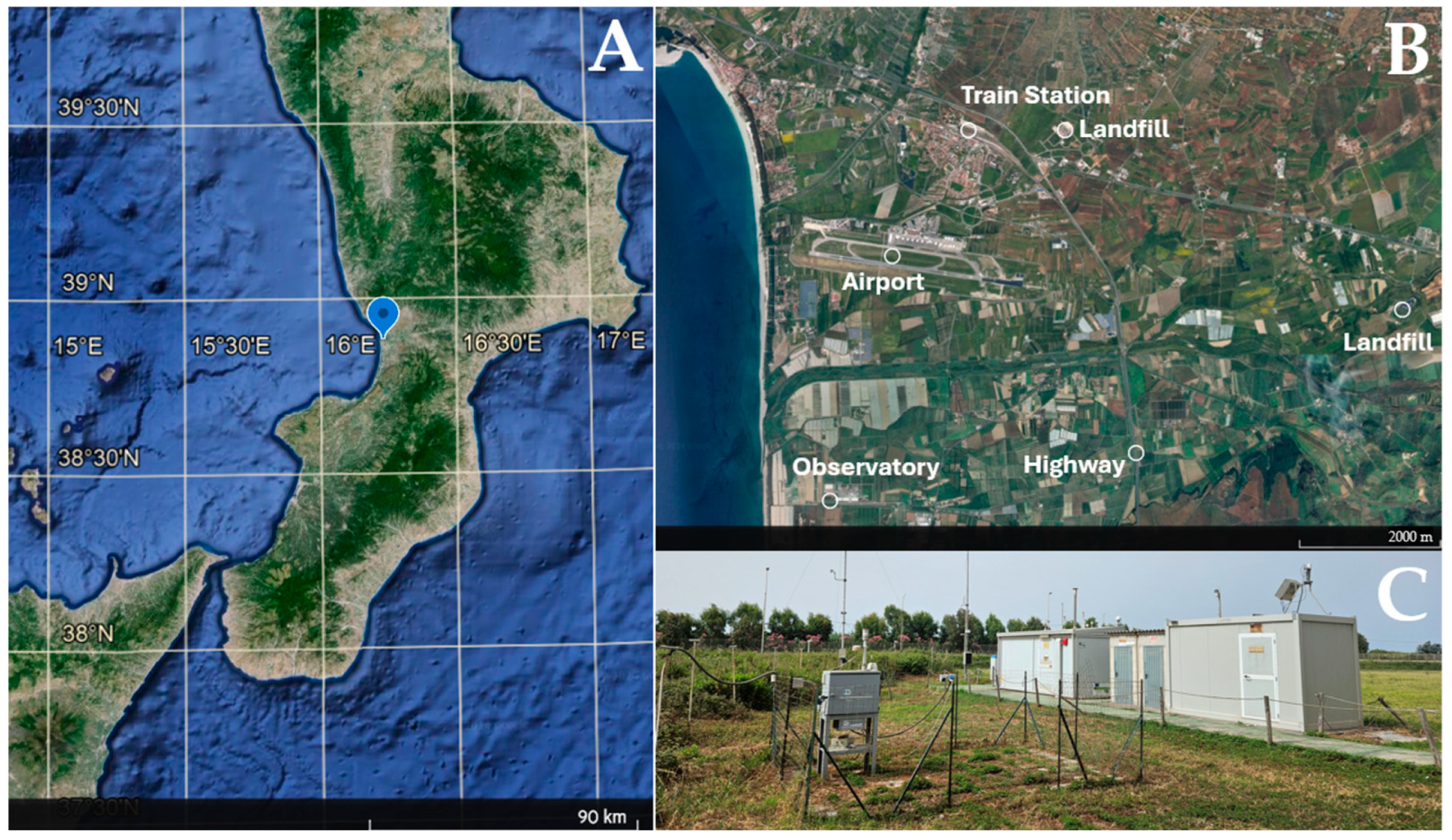
2. The Lamezia Terme CNR-ISAC Observatory

The Lamezia Terme site (WMO/GAW code: LMT) is a coastal station located in Calabria, Southern Italy, more precisely, in the Sant’Eufemia plain (Lat: 38.88° N; Lon: 16.23° E; Alt: 6 m above sea level), south of Lamezia Terme. The observatory, fully operated by the National Research Council of Italy-Institute of Atmospheric Sciences and Climate (CNR-ISAC), is located approximately 600 m from the Tyrrhenian coastline of Calabria, and officially started its data gathering operations in 2015. It has since provided continuous data on several chemical and meteorological parameters. Wind characteristics at this coastal site were analyzed in the past [29]. Due to the geographic location of the experimental site, winds coming from the northeast are more subject to anthropogenic influence while winds coming from the west, largely influenced by the sea, yield lower concentrations in pollutants, as clearly demonstrated in an earlier study [30]. The prevailing W-NE local wind circulation is well established in sectors other than atmospheric research: in fact, the magnetic bearing of the runway in use at the nearby Lamezia Terme International Airport (IATA: SUF; ICAO: LICA) is 10/28 (100–280° N).

Ever since it started operations, LMT reported methane concentrations that may be attributable to several nearby sources, hence the concept of a “multisource” coastal site. Cristofanelli et al. (2017) [30], accounting for one year of data gathering, indicated the nearby Lamezia Terme International Airport (located 3 km north from the observation site) and local livestock farming as two possible explanations for the observed peaks in methane, in addition to the anthropogenic pollution from nearby urban areas that is channeled towards the observatory when winds are coming from the northeast, as well as the A2 highway (part of the European route E45) located nearby (Figure 1B). In addition to the above-mentioned sources, it is worth noting the presence of Lamezia Terme Centrale (Lamezia Terme Central Station), which is a hub for railway connections between the main Tyrrhenian/cross country line and the Ionian line on the opposite coast of the region. The train station is located 5.4 km N-NE of LMT. Two landfills are also located nearby, and their locations are marked in Figure 1B. Farms are spread over the area.

From a climatological point of view, the area is known to be affected by seasonal changes to wind circulation. The study area, due to its geographical location, is mainly affected by breeze circulation, as assessed by several works.

Federico et al. (2010a) [29], in studying the characteristics and importance of breezes, demonstrated how they dominate the local circulation and play a major role in the local climate. The authors observed relevant changes in average wind speeds over the seasons, as well as slight changes in wind orientation, though the general W-WSW/NE-ENE axis is dominant throughout the whole year and is deemed the result of wind channeling through the Marcellinara gap, which is the narrowest point in the entire Italian peninsula. When the 850 hPa layer is considered, the preferred orientation switches to a prevailing NW direction, which is consistent with large scale circulation in the area. Federico et al. (2010b) [31] further analyzed the nature of breeze circulations, considering two years of observation and modeling analyses, concluding that during spring, summer, and part of fall, diurnal breeze circulation is considered as a combination of local and large-scale flows, while large-scale forcing represents a main driver of diurnal circulation in winter, November included, and nocturnal flows are believed to be due to the circulation of nocturnal breezes.

The confirmation on the presence of breeze and the influence of local conditions were both confirmed by further studies such as Gullì et al. (2017) [32] via the analysis of wind–lidar profiles for two continuous years. Figure 2 shows wind profiles accounting for multiple altitude thresholds, from 10 up to 300 m, collected by a Zephir Lidar 300 at the LMT observation site.

In a recent work, Lo Feudo et al. (2020) [33] studied the characteristics of the vertical structure of the Planetary Boundary Layer (PBL) at the LMT site during an experimental campaign carried out in July/August 2009. The integration of different instruments (surface stations, wind profiler, lidar, and sodar) with high resolution weather model products allows researchers to further assess the roles played by sea breeze and synoptic flows in the area.

Due to its location in the articulated context of the Mediterranean and, specifically, in the narrowest corridor of the Italian peninsula, the LMT station is subject to exposure to open fire emissions, as recently reported in Malacaria et al. (2024) [34], and frequent Saharan dust events [35].

3. Instruments, Datasets, and Methods

Data on methane (ppb) mole fractions have been gathered by a Picarro G2401 CRDS (Cavity Ring-Down Spectrometry) analyzer (Santa Clara, CA, USA). This high-precision instrument measures gas concentrations in the atmospheric medium thanks to their capacity to absorb and scatter light at specific wavelengths, which ensures high-precision estimates on mole fractions. The same instrument also gathers data on CO (carbon monoxide, in ppm), CO₂ (carbon dioxide, in ppm), and H₂O (water vapor, as a percentage). Specifically, the G2401 CRDS analyzer operates via a four-point configuration: one gathers ambient air, while the other three are connected to three standard calibration cylinders produced by the WMO/GAW Central Calibration Laboratory hosted by NOAA (National Oceanic and Atmospheric Administration) GML (Global Monitoring Laboratory) to ensure comparability with the WMO X2004 mole fraction scale. The reference cylinders cover CH₄ fractions in the 300–2600 nmol/mol range. A Vici-Valco rotative valve (model: EMTMA-CE) switches between the four configurations at regular intervals. In particular, calibration cylinders are measured every 14 days. Each cylinder is measured for a time span of 30 min during three measurement cycles (360 min). Furthermore, three target cylinders are measured for quality check purposes every 19 h. A Nafion dryer (model: MD-070-144S-4) reduces the impact of water vapor on measurements by drying ambient air. Dried air is then analyzed by the G2401. Measurements occur every 5 s with a precision of 1 ppb. For the purpose of this research, hourly averages have been considered and their respective standard deviations are reported throughout this article.

An automatic weather station (Vaisala WXT520, Vantaa, Finland) measured at 10 m ASL the following meteorological parameters: temperature, relative humidity, wind speed and direction, pressure, and rain (10 averaged minutes). For the purposes of this research, wind speed and wind directions have been considered and are measured by the WXT520 instrument via ultrasound. Wind speed data have an uncertainty of ±0.3 m/s, while wind direction data have an uncertainty of ±3 sexagesimal degrees. Wind data, just like in the previous case, have been aggregated on an hourly basis featuring the standard deviation as a data stability indicator.

Table 1. Main coverage parameters (expressed as percentage of total actual hours per year) of the entire dataset spanning seven years of continuous observations at LMT are shown in this table. Also reported is the coverage rate per year, with a maximum total coverage of 99.57% in 2017, and a minimum coverage of 83.83% in 2022. The second column shows the integration of Picarro G2401 and Vaisala WXT520 data satisfying the condition where both instruments were reliably operating at the same time.

Year	Picarro Coverage (%)	Picarro-Vaisala (%)
2016	94.92%	92.2%
2017	99.57%	93.37%
2018	94%	74.68%
2019	97.6%	97.57%
2020	93.8%	93.79%
2021	97.71%	97.46%
2022	83.83%	75.41%
	94.49% 1	89.07% 1

¹ Total coverage.

shows the coverage of available methane data compared to the total amount of hours elapsed between 1 January 2016 and 31 December 2022 (61,368). Overall, of the 61,368 elapsed hours, 57,990 (94.49%) have been covered by verified and calibrated methane detections. This dataset will be referred to as “primary” throughout the paper. Three years out of seven have a total coverage rate exceeding 95%. Please note that both 2016 and 2020 are leap years, with an extra 24 h each (8784 h instead of 8760).

Table 1 also reports the overall coverage of Picarro G2401 and Vaisala WXT520 data compared to the actual number of hours of the entire observation period. Data analysis involving both chemical data on methane and meteorological wind data was based on a subset of the main database where both instruments were fully operating at the same time. This, by definition, led to a slightly smaller “secondary” dataset available for cross-analyses of this particular kind. Five out of seven years have a combined integrated data coverage of more than 90%.

Finally, the two datasets have been processed in R 4.4.0 via ggplot2, ggpubr, tidyverse, and openair packages, as well as their respective libraries. Depending on the purpose of each analysis, data have also been aggregated on a seasonal basis (JFD = December, January, February for Winter; MAM = March, April, May for Spring; JJA = June, July, August for Summer; SON = September, October, November for Fall). Yearly, monthly, and daily aggregations have also been computed.

4. Results

4.1. General Monthly Trend

The longer dataset compared to previous research [30] highlights more long-term trends and cycles. Figure 3 shows monthly aggregated averages where seasonal trends, as well as a general upward trend, can be noticed. The 1st and 3rd quartiles are also plotted in Figure 3. Higher values are generally linked to Winter and Fall seasons, while Summer and Spring seasons yield the lowest values per year. A November 2017 peak can be noticed in pre-pandemic years and will be discussed in Section 5.

4.2. Daily Cycle

With respect to daily cycles, intended as variations over the course of 24 h, Figure 4 shows the hourly variation of methane mole fractions. The figure shows seasonal 2019 data specifically, as it is the year with the highest degree of integrated methane and wind data coverage (97.57%, see Table 1). Data are from the primary dataset.

Table 2. The hourly values plotted in Figure 4 are listed, with the addition of standard deviations for each seasonal parameter. The table refers specifically to 2019.

Hours	Winter	Win. SD	Spring	Spr. SD	Summer	Sum. SD	Fall	Fa. SD
0	2076.27	163.49	2030.78	99.30	2066.69	113.04	2043.76	86.57
1	2076.78	157.14	2036.03	110.72	2078.96	118.00	2065.42	138.91
2	2087.11	162.39	2054.75	136.81	2084.67	124.21	2069.45	107.13
3	2082.18	161.63	2057.92	152.80	2102.78	130.50	2078.47	116.90
4	2087.75	174.86	2054.98	154.43	2088.88	123.60	2091.81	141.44
5	2079.08	156.14	2070.65	150.94	2086.37	122.84	2100.68	143.55
6	2089.18	167.36	2043.86	115.58	2045.54	100.81	2080.75	121.62
7	2096.24	178.82	2002.39	91.74	1980.23	57.72	2058.33	105.30
8	2043.12	120.53	1966.65	48.25	1943.77	26.59	1997.36	57.00
9	1994.23	90.90	1953.08	24.33	1933.72	16.59	1961.31	34.57
10	1964.34	38.20	1948.24	15.71	1931.18	14.27	1950.67	25.13
11	1955.17	27.22	1947.67	15.55	1929.20	14.54	1945.88	27.87
12	1953.52	24.69	1947.42	15.17	1926.67	13.62	1943.12	19.89
13	1952.92	25.71	1945.74	13.58	1925.17	14.20	1941.48	17.17
14	1951.27	17.15	1944.92	13.12	1925.21	15.02	1940.85	17.86
15	1952.23	18.01	1946.33	14.14	1924.65	14.22	1941.62	16.52
16	1956.75	24.34	1946.45	15.31	1924.85	14.36	1945.54	21.89
17	1967.86	38.03	1947.92	16.32	1926.58	19.07	1961.88	45.35
18	1979.94	49.42	1951.55	19.72	1928.99	31.05	1985.03	71.06
19	1994.36	65.39	1970.26	41.22	1938.43	40.10	1994.08	62.93
20	2009.53	83.48	1985.83	60.23	1977.44	92.46	2006.87	76.47
21	2030.08	102.69	2003.80	80.21	2019.90	111.61	2022.63	82.51
22	2046.53	124.62	2024.07	94.40	2033.38	115.17	2024.07	85.05
23	2051.48	135.37	2023.57	87.10	2051.06	114.79	2042.95	95.66

reports the average values per hour, divided by season, as well as the standard deviations computed during data evaluation. Data and graphs concerning years other than 2019 are available as Supplementary Materials S1(A1) through S1(F3): the y axis of these graphs is set to the same scale to allow direct comparisons between years. Figure 4(A2,B2) have a different scale compared to A1,B1 meant to visualize the daily cycle both in terms of absolute concentrations (A2) and standard deviations (B2).

Overall, a prominent daily cycle is reported in Figure 4. Seasonal differences can also be noticed, with the Winter and Summer seasons yielding the highest and lowest values, respectively, though this does not occur throughout the entire observation period. The “flat valley” in both absolute methane concentrations and hourly standard deviations occurring between 10:00 and 16:00 UTC is no coincidence, as the influence of local wind circulation on observed concentrations is known to be substantial. This interval coincides, in fact, with prevalent SW-NW sectors. At 03:00 UTC, the standard deviations are in the 116.9–161.63 ppb range (Fall and Winter, respectively), while at 15:00 UTC, the range is 14.14–18.01 ppb. Identical graphs and tables, though applied to the other years, are accessible as Supplementary Materials S1A through S1G. Graphs showing the variations in standard deviations are also accessible from these materials.

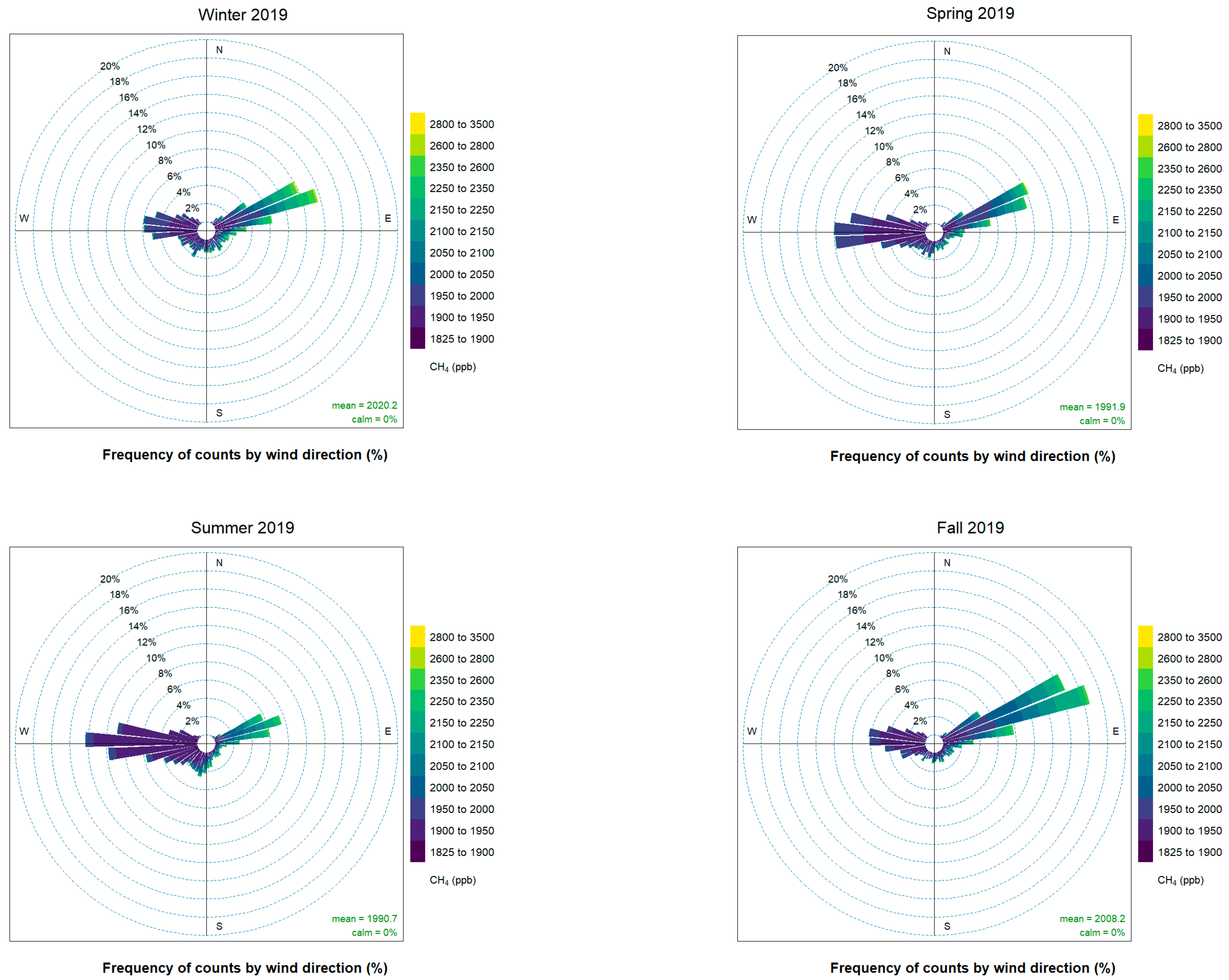
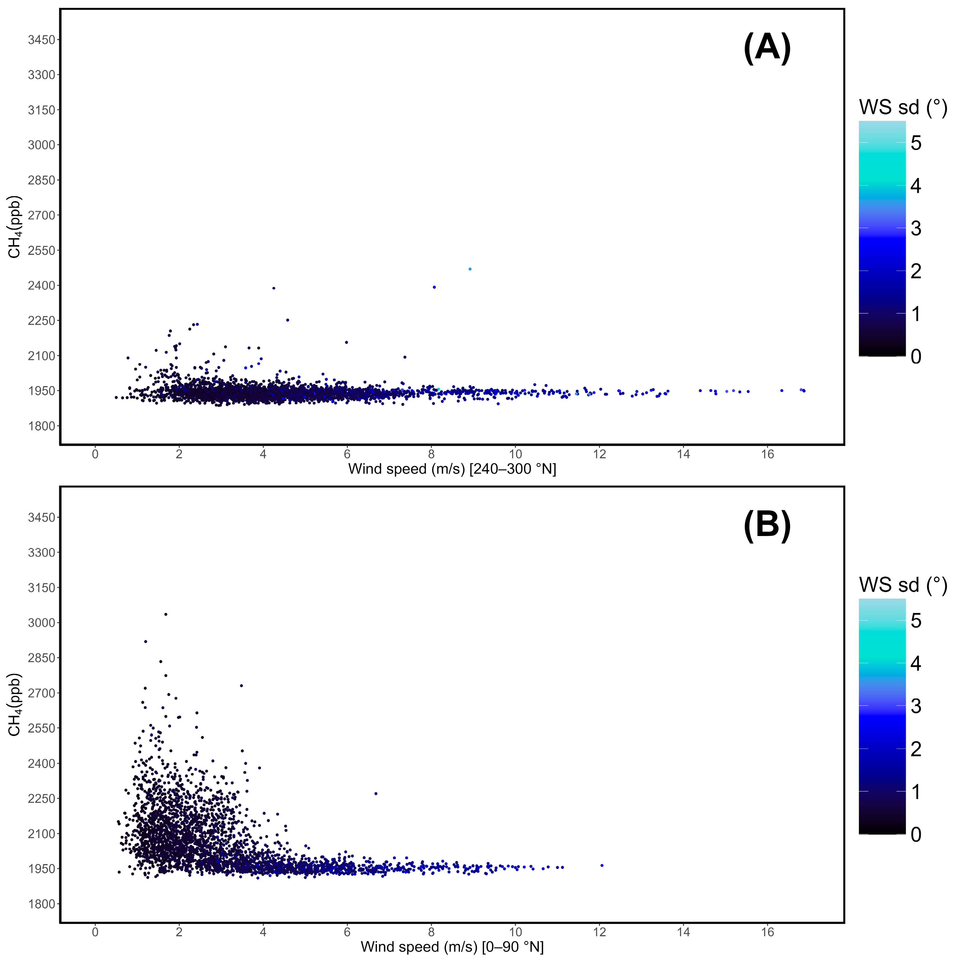
4.3. Wind Data Evaluation

Pollution roses referring to 2019 are shown in Figure 5, grouped by season. For these evaluations, the secondary dataset described in Table 1 was used. As reported in Section 2, the observation site is affected by two distinct wind circulation corridors: a pure western-seaside sector yielding generally lower methane concentrations, and a northeastern-continental sector showing much higher concentrations. Pollution roses reporting data referring to the other years are accessible as Supplementary Materials S2A through S2F.

Via the application of two distinct filters, observed methane concentrations have been correlated with wind speeds. In particular, a western-seaside sector (240–300° N, 3260 h) and a northeastern-continental (0–90° N, 2921 h) sector have been filtered from the secondary dataset, constituting, respectively, 38.13% and 34.17% of 2019’s available data. An amount of 27.7% of detections fall outside these ranges. The results are shown in Figure 6 and clearly indicate how the highest methane concentrations are linked to northeastern winds, in conjunction with lower wind speeds (Figure 6B). Winds coming from the west sector yield considerably lower methane concentrations, even though wind speeds are variable and winter-time peaks exceeding 14 m/s can be noticed (Figure 6A). Also, note how—if combined—the two sectors would lean to a hyperbola branch distribution, as shown in Supplementary Material S3G (the supplementary graph also includes values falling outside the two ranges). Supplementary Materials S3A through S3F show the same graphs applied to years other than 2019, while S3G shows all observed values.

4.4. Outbreak Analysis

A further evaluation was aimed specifically at possible indicators of anthropogenic activities, which could be susceptible to weekdays, under the assumption that no natural mechanism would lead to substantial statistical differences affecting the occurrence of outbreak events during a week. In the case of 2019, two distinct evaluations have been performed on a per-weekday basis, one accounting for values equal to or greater than the 3rd quartile (2029.11 ppb), and a second, more constrained evaluation accounting for the top 2.5% values (2299.91 ppb). The analysis was performed on the primary Picarro G2401 dataset. Respectively, 2138 and 214 h satisfied these conditions, now plotted in Figure 7. Supplementary Materials S4-A through S4-F show results concerning years other than 2019.

Table 3. The 3rd quartile and 97.5% threshold counts data and details, per year. The last row shows the total number of hours exceeding the two limits, as well as the average count of hours satisfying that condition, by weekday.

Year	3rd Q. (ppb)	Hours ≥ 3rd Q.	Average Count Per Weekday (3rd Q.)	97.5% Threshold (ppb)	Hours ≥ 97.5% Threshold	Average Count per Weekday (97.5%)
2016	1994.2	2085	297.85	2418.76	209	29.85
2017	2031.23	2181	311.57	2401.73	219	31.28
2018	2017.44	2059	294.14	2346.05	206	29.42
2019	2029.11	2138	305.71	2299.91	214	30.57
2020	2056.46	2060	294.28	2278.84	206	29.42
2021	2069.5	2140	305.71	2337.82	214	30.57
2022	2117.58	1836	262.28	2432.91	184	26.28
		14,499 1	2071.28 2		1452 1	207.42 2

¹ Total amount. ² Average value.

shows the two filters, including the number of hours satisfying their conditions, throughout the entire 2016–2022 period.

A Chi-squared test was performed on combined data concerning outbreak events listed by weekday. Said test was executed in R 4.4.0 by setting a value of 9999 Monte Carlo replicates.

Table 4. Results of the Chi-squared test performed to verify the possible outbreak occurrence susceptibility to specific weekdays. For the graph, see Supplementary Material S4G.

Type	Average	MON	TUE	WED	THU	FRI	SAT	SUN	χ2	p-Value
3rd Q.	2071.28	1899	2024	2089	2163	2246	2082	1996	37.152	0.0001
97.5% th.	207.42	181	179	210	201	251	207	223	17.817	0.0064

reports the data used, as well as the computed χ² and p-values for both the 3rd quartile and 97.5% threshold. For the graph, see Supplementary Material S4G. Though over the course of the observation period, a variability in peaks per weekday can be noticed (see Supplementary Materials S4A through S4F), combined 2016–2022 data point to Friday as the weekday with the most frequent occurrence of outbreaks. Due to its higher χ² and lower p-value, the 3rd quartile category has provided a more statistically relevant result in terms of distribution.

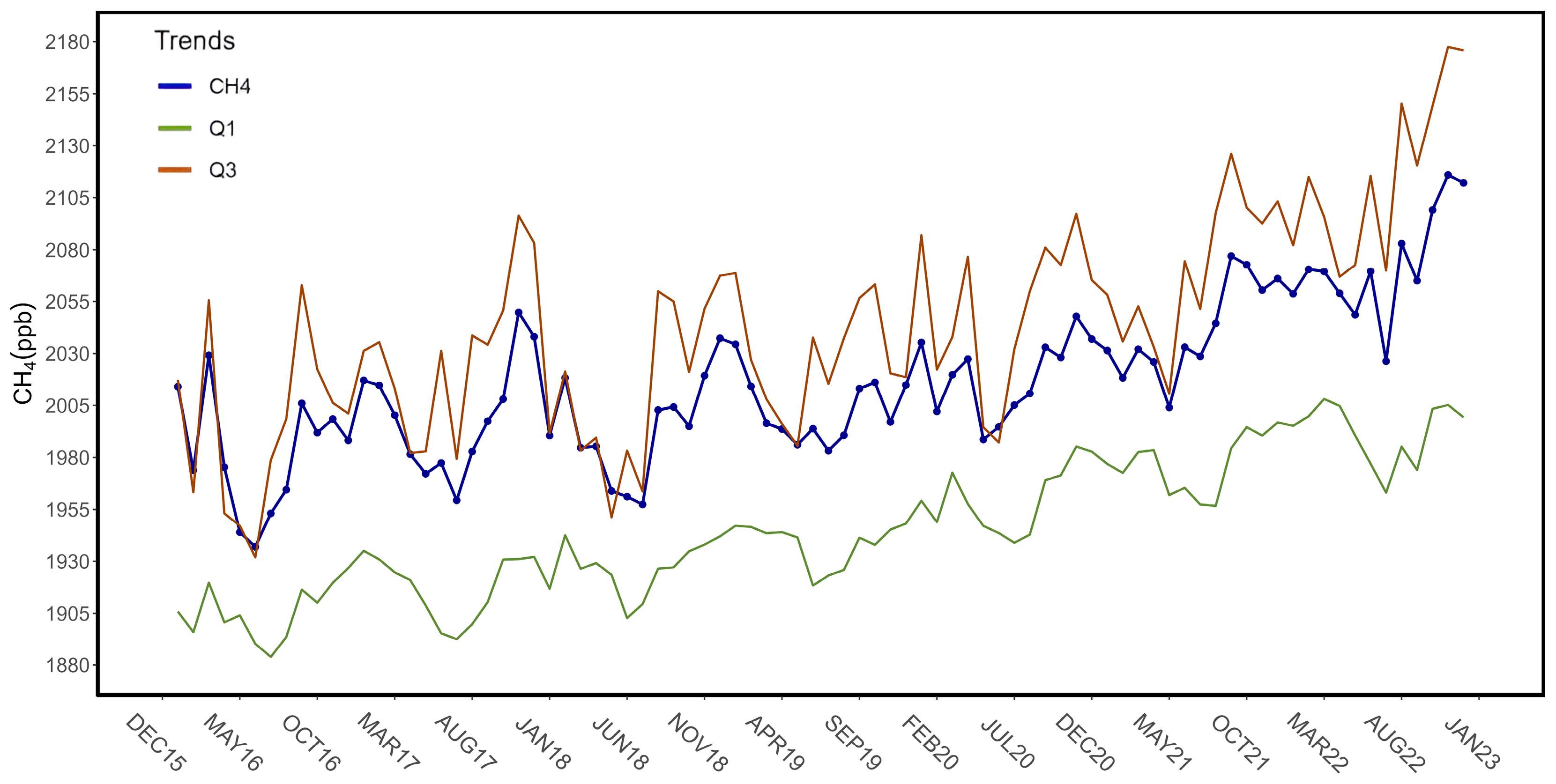
4.5. Multi-Year Trend

Finally, a multi-year trend has been plotted in Figure 8. For this evaluation, the year 2022 has been excluded due to its lower coverage rate of 83.83% compared to the other years, which fall in the 93.8–99.57% range (see Table 1).

The global annual means issued by NOAA and LMT’s observations have been compared. Differences between annual means are shown in

Table 5. Annual means of methane concentrations and their respective standard deviations, in ppb. The year 2022, written in italics, is excluded from Figure 7 and Figure 8. NOAA annual means and changes are extrapolated from Lan et al. (2024) [36].

Year	CH4 (ppb)	CH4 SD (ppb)	Coverage (%)	Change (ppb)	NOAA (ppb)	NOAA Change (ppb)	LMT-NOAA Diff. (ppb)
2016	1980.87	146.78	94.92	-	1843.12	+7.05	137.75
2017	1999.75	140.30	99.57	+18.88	1849.67	+6.89	150.08
2018	1994.88	121.38	94	−4.87	1857.33	+8.70	137.55
2019	2002.50	106.98	97.6	+7.62	1866.58	+9.67	135.92
2020	2018.79	96.20	93.8	+16.29	1878.93	+15.17	139.86
2021	2040.79	105.99	97.71	+22.00	1895.28	+17.91	145.51
2022 1	2074.87	126.87	83.83	+34.07	1922.53	+13.26	137.75

¹ 2022 is reported in italics but not featured in Figure 8 and Figure 9.

. Overall, with the exception of a surge in 2017 (difference: 150.08 ppb), five annual differences in the 2016–2021 period fall in the 135.92–139.86 ppb range, with the 2022 divergence being identical to that of 2016. Both trends are shown in Figure 9.

Both Table 5 and Figure 9 remark on the 2020 surges, which are likely related to the COVID-19 pandemic, which is known to have led to an increase in global CH₄ concentrations [36,37], though other factors need to be considered to justify these surges (see Section 5). On average, LMT annual means exceed the global NOAA values by 141.11 ppb. The 2017 surge is local, and further information on 2017 trends can be obtained via Supplementary Materials S1(B1), S1(B2), S1(B3) (daily cycles), S2B (seasonal pollution roses), and S3(B1), S3(B2) (wind speed and mole fractions).

5. Discussion

The larger dataset and the integration of key meteorological information have allowed for a more detailed analysis on methane concentrations detected at the LMT observatory. The detailed analysis on methane detections from the 0–90° N range allows researchers to better constrain some of the hypotheses made in the past on local sources of pollution and integrate them with new hypotheses. Research such as Cristofanelli et al. (2017) [30] proposed local livestock farming, air traffic, domestic heating (Winter-specific), and landfills among the causes of higher GHG and reactive gas concentrations in the area. In the case of methane, this is compatible with observed wind directions at LMT, as the locations of at least one landfill, the A2 highway, nearby urban areas, and specific take-off/landing trajectories at SUF/LICA airport, are indeed compatible with these wind regimes, methane peaks, and their respective seasonal variations.

The general trend seen in Figure 3 highlights seasonal cycles and an upward trend towards higher concentrations over time, while the daily cycles seen in Figure 4 are dominated by wind circulation. “Flat valleys” in hourly graphs are linked to western winds. The further analysis of methane concentrations with respect to wind directions (Figure 5) and speed (Figure 6) has allowed us to determine the existence of two main corridors: a western-seaside direction, linked to lower methane concentrations regardless of wind speed, and a northeastern-continental direction, which is characterized by higher methane mole fractions (especially in the case of low wind speeds), which are likely due to nearby sources of this compound. The corridors are susceptible to seasonal variations, as reported in Figure 5 and related Supplementary Materials.

For the first time in the data-gathering history of the observation site LMT, a possible correlation between weekdays and outbreak events was tested under the assumption that no mechanism in nature other than anthropogenic factors would lead to statistically significant differences in outbreak event occurrence over the course of weekdays. Figure 7 and Table 4, as well as related Supplementary Materials S4A through S4G, provide statistical relevance to higher results on Fridays, though it is worth noting that each year’s results show several degrees of variability. Friday peaks may be the result of additional anthropogenic emissions related to commuting, public transportation, farming, and industrial activities, though future works will have to investigate these occurrences even further. A previous study on black carbon (BC), PM_2.5, and PM₁₀ concentrations already reported higher weekday/weekend ratios as an indicator of additional anthropogenic activity [38].

Overall, the results shown in this work with respect to methane concentration variability depending on wind direction, combined with the statistical distribution of outbreaks over the course of weekdays, seem to corroborate the hypothesis seen in previous studies such as Cristofanelli et al. (2017) [30] by which anthropogenic sources located in the northeast with respect to LMT are responsible for generally higher methane concentrations in the area. In the context of a “multisource” scenario, the previous study reported, in particular, two possible sources of methane in the area: local livestock farming and air traffic. A case can be made, following the research by Malacaria et al. (2024) [34], that wildfires also constitute methane sources affecting LMT detections, but this needs to be corroborated by future research, possibly accounting for additional atmospheric tracers. These findings could then be used by regulators and policy makers to address issues related to local air quality concerns.

Livestock such as cattle are indeed responsible for major methane emission levels worldwide [39,40] and contribute up to an estimated 14.5% of total anthropogenic greenhouse gas emissions. Specifically, Hristov et al. (2013) [41] reported that each cow releases 60–160 kg CH₄ y⁻¹, while goats and sheep release 10–16 kg CH₄ y⁻¹, all depending on characteristics such as the dry matter intake parameter (DMI) and size of the ruminant. In the case of observed methane concentrations at LMT, it is currently impossible to pinpoint emissions strictly related to livestock farming in the area unless new parameters such as carbon isotope fractionation are considered. This extra parameter will discriminate livestock methane from fossil fuel output and other sources of this compound.

Similarly, the influence of local air traffic is also difficult to estimate for a number of reasons, including operational characteristics and aeronautical procedures. One preliminary conclusion would be that the observatory and the airport’s runways intersect two parallel air corridors which do not affect each other, but the leading literature on air traffic pollution and emissions place the LMT station inside the “near-airport” (<10 km) range category, which is—according to studies such as Carslaw et al. (2006) [42] and Carslaw and Beevers, (2013) [43]—subject to direct air traffic influence. Aircraft engine combustion processes are among the known sources of methane and do contribute to anthropogenic climate change [44,45]. The literature on air quality perturbation by air traffic has also focused on LTO (landing to take-off) cycles, which are related to operational phases during which aircraft are either on the ground or at low altitudes [46,47], while research on broader effects of air traffic also considers cruise phases [48,49]. The airport was recognized in previous research as a possible influence over LMT’s detections [30], but no source apportionment has been performed. Specifically, runway (RWY) 10 take-offs (aircraft facing east) and RWY 28 landings (aircraft facing west) would place aircraft on trajectories compatible with the northeastern-continental wind sector shown in Figure 5 and related Supplementary Materials. It is presently not possible, without the introduction of additional tracers, to provide tangible estimates concerning the airport’s influence over local methane detections.

Finally, relevant assumptions can be made when considering multi-year trends observed at LMT. Globally, methane concentrations are on the rise as a result of anthropogenic activities, natural emissions (e.g., wetlands), and major variations in sinks [26,36]. On a local scale—though the clear upward trend persists—sporadic “bursts” of concentrations may occur, such as the 2017 peak reported in Figure 8, Figure 9, and Table 5. In the case of LMT, November 2017 yields a peak average value of 2049.74 ± 178.2 ppb (mean ± 1σ), which does not have a clear explanation. Supplementary Materials S1(B1), S1(B2), S1(B3) (daily cycles), S2B (seasonal pollution roses), and S3(B1), S3(B2) (wind speed and mole fractions), all referring to 2017, point to higher concentrations from the NE sector, that we attributed mainly to anthropogenic activities. However, it is not possible to pinpoint specific emission sectors linked to these peaks; we do exclude wildfires as a possible source due to the season involved (Fall). In 2020, a year heavily affected by the COVID-19 pandemic, global values experienced a 15 ppb increase [14,36], which is similar to the 16.29 ppb surge observed at LMT. It is worth noting that an annual global increase of 1 ppb is believed to be the result of an extra ≈2.77 Tg CH₄ being emitted into the atmosphere [5]. The 2019–2020 local-to-global leap is not surprising, as the COVID-19 outbreak lockdowns are among the causes of increases in methane concentrations [37]. Methane has a latency of approximately one decade in the atmosphere, but several models clearly show that the peak response of this alkane occurs within a few months from extra-emission pulses [50,51], corroborating the hypothesis by which the 2020 peak is at least partially linked to nation-wide lockdowns and consequent increases in emissions from the energy sector [52], though the 2020 peak is likely due to a combination of multiple factors. A recent study by Feng et al. (2023) [53] estimated that 66% of the 2020 methane surge was due to increased emission rates, though it is worth noting that changes in sinks caused by reduced NO_x have also been reported as leading causes for such surges [26]. Also, although on the global scale an upward trend is detected, findings at the LMT observation site confirm concentration levels that are also dependent on latitude and hemisphere [19,20], which would explain why LMT yearly trends follow a pattern similar to that of global trends observed by NOAA (Figure 9), with a difference in terms of absolute concentrations that is also driven by its geographical context and fluxes occurring at local and regional scales.

Moreover, it is worth specifying that CH₄ reacts with the hydroxyl radical (OH), which is the main compound responsible for methane sink in natural environments [54,55]. The hydroxyl is not directly measured at LMT, so direct comparisons and correlations between the trends of both compounds are not possible. It is recognized, however, that the availability and diffusion of hydroxyl is a major controlling factor for methane and is, therefore, responsible for net atmospheric increases and losses [7], though several uncertainties in its trends and quantifications exist [56]. Exceptional events such as the VEI-6 eruption of Mount Pinatubo in 1991 and the consequent release of SO₂ and sulfates in the atmosphere have reportedly reduced the sink of CH₄ from reaction with OH in the troposphere by approximately 17.8 Tg between June 1991 and June 1993 [57]. Chlorine also contributes to active methane removal from the atmosphere and estimates such as those proposed by Hossaini et al. (2016) [58] provide an approximate value of 12–13 Tg y⁻¹, though further research indicates that this sink may be less than half than that [59]. Despite its minor role, the chlorine sink has a strong isotopic fingerprint which can be determined via adequate equipment and instruments [60,61]. Future research at LMT, accounting for the carbon isotope fractionation of methane, could potentially provide information on the influence of the chlorine sink. Furthermore, by contrast to methanogenesis induced by microbial activity [62], methanotroph bacteria in water and soils also contribute to the removal of methane [63,64], but as soils are constantly threatened by human activities [65], forest soils’ methane uptake capacity is also compromised, especially considering the fact that it is already vulnerable to environmental factors such as precipitation [66]. There is, however, evidence going in the opposite direction, with consistent reports of increasing forest soil methane uptake [20]. Trends aside, these drivers of methane removal help reduce to nearly one decade the latency of this compound in the atmosphere, while carbon dioxide can persist for several centuries, at most, one millennium [3]. At least in the case of the hydroxyl radical, it has been demonstrated that post-2006 methane atmospheric increases cannot be solely attributed to a decrease in atmospheric OH [14], thus adding up even more to the general complexity of methane buildup into the atmosphere. The complexity behind the interaction of methane with the hydroxyl radical, therefore, requires more research be aimed at the investigation of sinks and their effects observed on CH₄ mole fractions.

6. Conclusions

For the first time, multi-year trends of methane detected by the Lamezia Terme WMO/GAW station (LMT) have been analyzed. Located close to the Tyrrhenian coast of Calabria, in the narrowest point of the Italian peninsula, measurements at this observatory are largely influenced by its peculiar location in the country. Daily cycles are influenced by local wind circulation and synoptic features: a western-seaside sector yields lower methane concentrations, while northeastern-continental winds yield the highest concentrations detected at LMT. The circulation is such that daytime winds come mostly from the western sector, thus resulting in much lower methane values, while nocturnal winds come from the northeast. Filtering data by wind direction clearly demonstrates the differences in terms of average concentrations as detected from the two sectors. Moreover, wind speed is also very closely tied to methane values, as the comparison of methane concentrations and wind speeds results in a hyperbola branch pattern where low speeds are linked to higher values and, vice versa, high speeds yielded lower values: this is interpreted as the influence of local emissions outputs. Seasonal differences and cycles are also well defined, with Winter and Summer seasons generally yielding the highest and lowest methane concentrations, respectively. Multi-year trends have been compared with NOAA’s global measurements: the upward tendencies are similar and differences between yearly averages fall mostly within a well-defined window (137.75–145.51 ppb; 2017 has a peak of 150.08 ppb), though it is worth noting that methane concentrations are known from the literature to vary depending on geographical factors such as latitude. For the first time, a method was introduced to correlate outbreak events of methane concentrations with weekdays in the effort to determine possible anthropogenic influences over these values, as these activities alone do have a weekly cycle which is totally lacking in nature. The results indicate that peaks tend to occur on Fridays, while Mondays and Sundays yielded lower values. The introduction of δ¹³C measurements of CH₄, as well as CO₂, would significantly help with source apportionment in future studies.

References

1. Byrom, R.E.; Shine, K.P. Methane’s Solar Radiative Forcing. Geophys. Res. Lett. 2022, 49, e2022GL098270. [Google Scholar] [CrossRef]
2. Myhre, G.; Shindell, D.; Bréon, F.M.; Collins, W.; Fuglestvedt, J.; Huang, J.; Koch, D.; Lamarque, J.F.; Lee, D.; Mendoza, B.; et al. Anthropogenic and Natural Radiative Forcing. In Climate Change 2013: The Physical Science Basis, Contribution of Working Group I to the Fifth Assessment Report of the Intergovernmental Panel on Climate Change; Intergovernmental Panel on Climate Change: Cambridge, UK; New York, NY, USA, 2013. [Google Scholar]
3. Sand, M.; Skeie, R.B.; Sandstad, M.; Krishnan, S.; Myhre, G.; Bryant, H.; Derwent, R.; Hauglustaine, D.; Paulot, F.; Prather, M.; et al. A multi-model assessment of the Global Warming Potential of hydrogen. Nat. Commun. 2023, 4, 203. [Google Scholar] [CrossRef]
4. Etheridge, D.M.; Steele, L.P.; Francey, R.J.; Langenfelds, R.L. Atmospheric methane between 1000 A.D. and present: Evidence of anthropogenic emissions and climatic variability. J. Geophys. Res. Atmos. 1998, 103, 15979–15993. [Google Scholar] [CrossRef]
5. Nisbet, E.G.; Manning, M.R.; Dlugokencky, E.J.; Fisher, R.E.; Lowry, D.; Michel, S.E.; Lund Myhre, C.; Platt, S.M.; Allen, G.; Bousquet, P.; et al. Very Strong Atmospheric Methane Growth in the 4 Years 2014–2017: Implications for the Paris Agreement. Glob. Biogeochem. Cycles 2019, 33, 318–342. [Google Scholar] [CrossRef]
6. Blunden, J.; Boyer, T.; Bartow-Gillies, E. State of the Climate in 2022. B. Am. Meteorol. Soc. 2023, 104, 1–501. [Google Scholar] [CrossRef]
7. Skeie, R.B.; Hodnebrog, Ø.; Myhre, G. Trends in atmospheric methane concentrations since 1990 were driven and modified by anthropogenic emissions. Commun. Earth Environ. 2023, 4, 317. [Google Scholar] [CrossRef]
8. Szopa, S.; Naik, V.; Adhikary, B.; Artaxo, P.; Berntsen, T.; Collins, W.D.; Fuzzi, S.; Gallardo, L.; Kiendler-Scharr, A.; Klimont, Z.; et al. Short-Lived Climate Forcers. In Climate Change 2021: The Physical Science Basis. Contribution of Working Group I to the Sixth Assessment Report of the Intergovernmental Panel on Climate Change; Masson-Delmotte, V., Zhai, P., Pirani, A., Connors, S.L., Péan, C., Berger, S., Caud, N., Chen, Y., Goldfarb, L., Gomis, M.I., et al., Eds.; Cambridge University Press: Cambridge, UK; New York, NY, USA, 2021; pp. 817–922. [Google Scholar]
9. Dlugokencky, E.J.; Steele, L.P.; Lang, P.M.; Masarie, K.A. The growth rate and distribution of atmospheric methane. J. Geophys. Res. Atmos. 1994, 99, 17021–17043. [Google Scholar] [CrossRef]
10. Saunois, M.; Bousquet, P.; Poulter, B.; Peregon, A.; Ciais, P.; Canadell, J.G.; Dlugokencky, E.J.; Etiope, G.; Bastviken, D.; Houweling, S.; et al. The global methane budget 2000–2012. Earth Syst. Sci. Data 2016, 8, 697–751. [Google Scholar] [CrossRef]
11. Saunois, M.; Bousquet, P.; Poulter, B.; Peregon, A.; Ciais, P.; Canadell, J.G.; Dlugokencky, E.J.; Etiope, G.; Bastviken, D.; Houweling, S.; et al. Variability and quasi-decadal changes in the methane budget over the period 2000–2012. Atmos. Chem. Phys. 2017, 17, 11135–11161. [Google Scholar] [CrossRef]
12. Saunois, M.; Stavert, A.R.; Poulter, B.; Bousquet, P.; Canadell, J.G.; Jackson, R.B.; Raymond, P.A.; Dlugokencky, E.J.; Houweling, S.; Patra, P.K.; et al. The Global Methane Budget 2000–2017. Earth Syst. Sci. Data 2020, 12, 1561–1623. [Google Scholar] [CrossRef]
13. Montzka, S.A. The NOAA annual greenhouse gas index (AGGI). NOAA Glob. Monit. Lab. 2023. Available online: https://gml.noaa.gov/aggi/aggi.html (accessed on 16 July 2024).
14. Lan, X.; Nisbet, E.G.; Dlugokencky, E.J.; Michel, S.E. What do we know about the global methane budget? Results from four decades of atmospheric CH4 observations and the way forward. Philos. Trans. A Math. Phys. Eng. Sci. 2021, 379, 20200440. [Google Scholar] [CrossRef] [PubMed]
15. IEA Methane Tracker 2021. International Energy Agency, Paris, 2021. Available online: https://www.iea.org/reports/methane-tracker-2021 (accessed on 16 July 2024).
16. Etiope, G.; Ciotoli, G.; Schwietzke, S.; Schoell, M. Gridded maps of geological methane emissions and their isotopic signature. Earth Syst. Sci. Data 2019, 11, 1–22. [Google Scholar] [CrossRef]
17. Chang, J.; Peng, S.; Ciais, P.; Saunois, M.; Dangal, S.R.S.; Herrero, M.; Havlík, P.; Tian, H.; Bousquet, P. Revisiting enteric methane emissions from domestic ruminants and their δ13CCH4 source signature. Nat. Commun. 2019, 10, 3420. [Google Scholar] [CrossRef] [PubMed]
18. Dlugokencky, E.; Nisbet, E.G.; Fisher, R.; Lowry, D. Global atmospheric methane: Budget, changes and dangers. Philos. Trans. A Math. Phys. Eng. Sci. 2011, 369, 2058–2072. [Google Scholar] [CrossRef] [PubMed]
19. Blake, D.R.; Mayer, E.W.; Tyler, S.C.; Makide, Y.; Montague, D.C.; Rowland, F.S. Global increase in atmospheric methane concentrations between 1978 and 1980. Geophys. Res. Lett. 1982, 9, 477–480. [Google Scholar] [CrossRef]
20. Yu, L.; Huang, Y.; Zhang, W.; Li, T.; Sun, W. Methane uptake in global forest and grassland soils from 1981 to 2010. Sci. Total Environ. 2017, 607–608, 1163–1172. [Google Scholar] [CrossRef] [PubMed]
21. Pison, I.; Ringeval, B.; Bousquet, P.; Prigent, C.; Papa, F. Stable atmospheric methane in the 2000s: Key-role of emissions from natural wetlands. Atmos. Chem. Phys. 2013, 13, 11609–11623. [Google Scholar] [CrossRef]
22. Dlugokencky, E.; Masarie, K.; Lang, P.; Tans, P.P. Continuing decline in the growth rate of the atmospheric methane burden. Nature 1998, 393, 447–450. [Google Scholar] [CrossRef]
23. Dlugokencky, E.J.; Houweling, S.; Bruhwiler, L.; Masarie, K.A.; Lang, P.M.; Miller, J.B.; Tans, P.P. Atmospheric methane levels off: Temporary pause or a new steady-state? Geophys. Res. Lett. 2003, 30, 1992. [Google Scholar] [CrossRef]
24. He, J.; Naik, V.; Horowitz, L.W.; Dlugokencky, E.; Thoning, K. Investigation of the global methane budget over 1980–2017 using GFDL-AM4.1. Atmos. Chem. Phys. 2020, 20, 805–827. [Google Scholar] [CrossRef]
25. Ferretti, D.F.; Miller, J.B.; White, J.W.C.; Etheridge, D.M.; Lassey, K.R.; Lowe, D.C.; Macfarling Meure, C.M.; Dreier, M.F.; Trudinger, C.M.; Van Ommen, T.D.; et al. Unexpected changes to the global methane budget over the past 2000 years. Science 2005, 309, 1714–1717. [Google Scholar] [CrossRef] [PubMed]
26. Peng, S.; Lin, X.; Thompson, R.L.; Xi, Y.; Liu, G.; Hauglustaine, D.; Lan, X.; Poulter, B.; Ramonet, M.; Saunois, M.; et al. Wetland emission and atmospheric sink changes explain methane growth in 2020. Nature 2022, 612, 477–482. [Google Scholar] [CrossRef]
27. Wilson, C. Untangling variations in the global methane budget. Nat. Commun. 2023, 4, 318. [Google Scholar] [CrossRef]
28. Padilla, R.; Adame, J.A.; Hidalgo, P.J.; Bolivar, J.P.; Yela, M. Short-term trend and temporal variations in atmospheric methane at an Atlantic coastal site in Southwestern Europe. Atmos. Environ. 2023, 333, 120665. [Google Scholar] [CrossRef]
29. Federico, S.; Pasqualoni, L.; De Leo, L.; Bellecci, C. A study of the breeze circulation during summer and fall 2008 in Calabria, Italy. Atmos. Res. 2010, 97, 1–13. [Google Scholar] [CrossRef]
30. Cristofanelli, P.; Busetto, M.; Calzolari, F.; Ammoscato, I.; Gullì, D.; Dinoi, A.; Calidonna, C.R.; Contini, D.; Sferlazzo, D.; Di Iorio, T.; et al. Investigation of reactive gases and methane variability in the coastal boundary layer of the central Mediterranean basin. Elem. Sci. Anth. 2017, 5, 12. [Google Scholar] [CrossRef]
31. Federico, S.; Pasqualoni, L.; Sempreviva, A.M.; De Leo, L.; Avolio, E.; Calidonna, C.R.; Bellecci, C. The seasonal characteristics of the breeze circulation at a coastal Mediterranean site in South Italy. Adv. Sci. Res. 2010, 4, 47–56. [Google Scholar] [CrossRef]
32. Gullì, D.; Avolio, E.; Calidonna, C.R.; Lo Feudo, T.; Torcasio, R.C.; Sempreviva, A.M. Two years of wind-lidar measurements at an Italian Mediterranean Coastal Site. In European Geosciences Union General Assembly 2017, EGU—Division Energy, Resources & Environment, ERE. Energy Procedia 2017, 125, 214–220. [Google Scholar] [CrossRef]
33. Lo Feudo, T.; Calidonna, C.R.; Avolio, E.; Sempreviva, A.M. Study of the Vertical Structure of the Coastal Boundary Layer Integrating Surface Measurements and Ground-Based Remote Sensing. Sensors 2020, 20, 6516. [Google Scholar] [CrossRef]
34. Malacaria, L.; Parise, D.; Lo Feudo, T.; Avolio, E.; Ammoscato, I.; Gullì, D.; Sinopoli, S.; Cristofanelli, P.; De Pino, M.; D’Amico, F.; et al. Multiparameter detection of summer open fire emissions: The case study of GAW regional observatory of Lamezia Terme (Southern Italy). Fire 2024, 7, 198. [Google Scholar] [CrossRef]
35. Calidonna, C.R.; Avolio, E.; Gullì, D.; Ammoscato, I.; De Pino, M.; Donateo, A.; Lo Feudo, T. Five Years of Dust Episodes at the Southern Italy GAW Regional Coastal Mediterranean Observatory: Multisensors and Modeling Analysis. Atmosphere 2020, 11, 456. [Google Scholar] [CrossRef]
36. Lan, X.; Thoning, K.W.; Dlugokencky, E.J. Trends in Globally-Averaged CH4, N2O, and SF6 Determined from NOAA Global Monitoring Laboratory Measurements. Version 2024-06, 2024. Available online: https://gml.noaa.gov/ccgg/trends_doi.html (accessed on 18 June 2024).
37. Laughner, J.L.; Neu, J.L.; Schimel, D.; Wennberg, P.O.; Barsanti, K.; Bowman, K.W.; Chatterjee, A.; Croes, B.E.; Fitzmaurice, H.L.; Henze, D.K.; et al. Societal shifts due to COVID-19 reveal large-scale complexities and feedbacks between atmospheric chemistry and climate change. Proc. Natl. Acad. Sci. USA 2021, 118, e2109481118. [Google Scholar] [CrossRef] [PubMed]
38. Donateo, A.; Lo Feudo, T.; Marinoni, A.; Calidonna, C.R.; Contini, D.; Bonasoni, P. Long-term observations of aerosol optical properties at three GAW regional sites in the Central Mediterranean. Atmos. Res. 2020, 241, 104976. [Google Scholar] [CrossRef]
39. Grossi, G.; Goglio, P.; Vitali, A.; Williams, A.G. Livestock and climate change: Impact of livestock on climate and mitigation strategies. Anim. Front. 2019, 9, 69–76. [Google Scholar] [CrossRef]
40. Tapio, I.; Snelling, T.J.; Strozzi, F.; Wallace, R.J. The ruminal microbiome associated with methane emissions from ruminant livestock. J. Anim. Sci. Biotechnol. 2017, 8, 7. [Google Scholar] [CrossRef]
41. Hristov, A.N.; Oh, J.; Firkins, J.L.; Dijkstra, J.; Kebreab, E.; Waghorn, G.; Makkar, H.P.S.; Adesogan, A.T.; Yang, W.; Lee, C.; et al. Special topics—Mitigation of methane and nitrous oxide emissions from animal operations: I. A review of enteric methane mitigation options. J. Anim. Sci. 2013, 91, 5045–5069. [Google Scholar] [CrossRef] [PubMed]
42. Carslaw, D.C.; Beevers, S.D.; Ropkins, K.; Bell, M.C. Detecting and quantifying aircraft and other on-airport contributions to ambient nitrogen oxides in the vicinity of a large international airport. Atmos. Environ. 2006, 40, 5424–5434. [Google Scholar] [CrossRef]
43. Carslaw, D.C.; Beevers, S.D. Characterising and understanding emission sources using bivariate polar plots and k-means clustering. Environ. Model. Softw. 2013, 40, 325–329. [Google Scholar] [CrossRef]
44. Lee, D.S.; Fahey, D.; Forster, P.M.; Newton, P.J.; Wit, R.C.N.; Lim, L.L.; Owen, B.; Sausen, R. Aviation and global climate change in the 21st century. Atmos. Environ. 2009, 43, 3520–3537. [Google Scholar] [CrossRef]
45. Lee, D.S.; Fahey, D.W.; Skowron, A.; Allen, M.R.; Burkhardt, U.; Chen, Q.; Doherty, S.J.; Freeman, S.; Forster, P.M.; Fuglestvedt, J.; et al. The contribution of global aviation to anthropogenic climate forcing for 2000 to 2018. Atmos. Environ. 2021, 244, 117834. [Google Scholar] [CrossRef] [PubMed]
46. Grobler, C.; Wolfe, P.J.; Dasadhikari, K.; Dedoussi, I.C.; Allroggen, F.; Speth, R.L.; Eastham, S.D.; Agarwal, A.; Staples, M.D.; Sabnis, J.; et al. Marginal climate and air quality costs of aviation emissions. Environ. Res. Lett. 2018, 14, 114031. [Google Scholar] [CrossRef]
47. Quadros, F.D.A.; Snellen, M.; Dedoussi, I.C. Regional sensitivities of air quality and human health impacts to aviation emissions. Environ. Res. Lett. 2020, 15, 105013. [Google Scholar] [CrossRef]
48. Barrett, S.R.H.; Britter, R.E.; Waitz, I.A. Global Mortality Attributable to Aircraft Cruise Emissions. Environ. Sci. 2010, 44, 7736–7742. [Google Scholar] [CrossRef] [PubMed]
49. Yim, S.H.L.; Lee, G.L.; Lee, I.H.; Allroggen, F.; Ashok, A.; Caiazzo, F.; Eastham, S.D.; Malina, R.; Barrett, S.R.H. Global, regional and local health impacts of civil aviation emissions. Environ. Res. Lett. 2015, 10, 034001. [Google Scholar] [CrossRef]
50. Wild, O.; Prather, M.J.; Akimoto, H. Indirect long-term global radiative cooling from NOx emissions. Geophys. Res. Lett. 2001, 28, 1719–1722. [Google Scholar] [CrossRef]
51. Stevenson, D.S.; Doherty, R.M.; Sanderson, M.G.; Collins, W.J.; Johnson, C.E.; Derwent, R.G. Radiative forcing from aircraft NOx emissions: Mechanisms and seasonal dependence. J. Geophys. Res. Atmos. 2004, 109, D17307. [Google Scholar] [CrossRef]
52. McNorton, J.; Bousserez, N.; Agustí-Panareda, A.; Balsamo, G.; Cantarello, L.; Engelen, R.; Huijnen, V.; Inness, A.; Kipling, Z.; Parrington, M.; et al. Quantification of methane emissions from hotspots and during COVID-19 using a global atmospheric inversion. Atmos. Chem. Phys. 2022, 22, 5961–5981. [Google Scholar] [CrossRef]
53. Feng, L.; Palmer, P.I.; Parker, R.J.; Lunt, M.F.; Bösch, H. Methane emissions are predominantly responsible for record-breaking atmospheric methane growth rates in 2020 and 2021. Atmos. Chem. Phys. 2023, 23, 4863–4880. [Google Scholar] [CrossRef]
54. Turner, A.J.; Fung, I.; Naik, V.; Horowitz, L.W.; Cohen, R. Modulation of hydroxyl variability by ENSO in the absence of external forcing. Proc. Natl. Acad. Sci. USA 2018, 115, 8931–8936. [Google Scholar] [CrossRef]
55. Zhao, Y.; Saunois, M.; Bousquet, P.; Lin, X.; Berchet, A.; Hegglin, M.I.; Canadell, J.G.; Jackson, R.B.; Deushi, M.; Jöckel, P.; et al. On the role of trend and variability in the hydroxyl radical (OH) in the global methane budget. Atmos. Chem. Phys. 2020, 20, 13011–13022. [Google Scholar] [CrossRef]
56. Nicely, J.M.; Canty, T.P.; Manyin, M.; Oman, L.D.; Salawitch, R.J.; Steenrod, S.D.; Strahan, S.E.; Strode, S.A. Changes in Global Tropospheric OH Expected as a Result of Climate Change Over the Last Several Decades. J. Geophys. Res. Atmos. 2018, 123, 10774–10795. [Google Scholar] [CrossRef]
57. Bândă, N.; Krol, M.; van Noije, T.; van Weele, M.; Williams, J.E.; Le Sager, P.; Niemeier, U.; Thomason, L.; Röckmann, T. The effect of stratospheric sulfur from Mount Pinatubo on tropospheric oxidizing capacity and methane. J. Geophys. Res. Atmos. 2015, 120, 1202–1220. [Google Scholar] [CrossRef]
58. Hossaini, R.; Chipperfield, M.P.; Saiz-Lopez, A.; Fernandez, R.; Monks, S.; Feng, W.; Brauer, P.; von Glasow, R. A global model of tropospheric chlorine chemistry: Organic versus inorganic sources and impact on methane oxidation. J. Geophys. Res. Atmos. 2016, 121, 14271–14297. [Google Scholar] [CrossRef]
59. Gromov, S.; Brenninkmeijer, C.A.M.; Jöckel, P. A very limited role of tropospheric chlorine as a sink of the greenhouse gas methane. Atmos. Chem. Phys. 2018, 18, 9831–9843. [Google Scholar] [CrossRef]
60. Saueressig, G.; Bergamaschi, P.; Crowley, J.N.; Fischer, H.; Harris, G.W. Carbon kinetic isotope effect in the reaction of CH4 with Cl atoms. J. Geophys. Res. Atmos. 1995, 22, 1225–1228. [Google Scholar] [CrossRef]
61. Lan, X.; Nisbet, E.G.; Dlugokencky, E.J.; Michel, S.E. Improved Constraints on Global Methane Emissions and Sinks Using δ13C-CH4. J. Geophys. Res. Atmos. 2021, 35, e2021GB007000. [Google Scholar] [CrossRef]
62. Le Mer, J.; Roger, P. Production, oxidation, emission and consumption of methane by soils: A review. Eur. J. Soil Biol. 2001, 37, 25–50. [Google Scholar] [CrossRef]
63. Hanson, R.S.; Hanson, T.E. Methanotrophic bacteria. Microbiol. Rev. 1996, 60, 439–471. [Google Scholar] [CrossRef]
64. Oh, Y.; Zhuang, Q.; Liu, L.; Welp, L.R.; Lau, M.C.Y.; Onstott, T.C.; Medvigy, D.; Bruhwiler, L.; Dlugokencky, E.J.; Hugelius, G.; et al. Reduced net methane emissions due to microbial methane oxidation in a warmer Arctic. Nat. Clim. Chang. 2020, 10, 317–321. [Google Scholar] [CrossRef]
65. Goldman, M.B.; Groffman, P.M.; Pouyat, R.V.; McDonnell, M.J.; Pickett, S.T.A. CH4 uptake and N availability in forest soils along an urban to rural gradient. Soil Biol. Biochem. 1995, 27, 281–286. [Google Scholar] [CrossRef]
66. Ni, X.; Groffman, P.M. Declines in methane uptake in forest soils. Proc. Natl. Acad. Sci. USA 2018, 115, 8587–8590. [Google Scholar] [CrossRef] [PubMed]
Figure 1. (A): The location of Lamezia Terme’s observation site within the region of Calabria, Southern Italy. (B): Details of the southwestern Lamezia Terme municipal area, with marks on the location of the observatory and key infrastructures/locations addressed in this research study, namely, SUF/LICA airport, the central train station, and two landfills. The “Highway” mark refers to a specific point to the east of LMT where the distance between the A2 highway itself and the observatory is approximately 4.3 km. Farms, including those with livestock, are spread over the area. (C): Details of the LMT observation site, where all instruments are located.
Atmosphere 15 00946 g001
Figure 2. Seasonal wind roses at all levels during the 2014–2016 period, divided by thresholds between 10 and 300 m, and collected by Zephir Wind Lidar. From Gullì et al. (2017) [32], modified.
Atmosphere 15 00946 g002
Figure 3. Monthly averages accounting for the entire 2016–2022 period (84 months), shown in dark blue. Attenuated brown and green lines show 3rd and 1st quartile trends, respectively.
Atmosphere 15 00946 g003
Figure 4. Hourly averages of methane concentrations, showing seasonal variations. The color scheme is the following: Winter (black), Spring (green), Summer (red), Fall (yellow). Please note that, as stated above, the graph is referring to 2019 data only. (A1): methane mole fractions; (A2): same data, with the y axis range narrowed down to highlight hourly changes; (B1): methane standard deviations; (B2): narrowed down graph.
Atmosphere 15 00946 g004aAtmosphere 15 00946 g004b
Figure 5. Seasonal pollution roses of methane concentrations observed at LMT and referring to 2019. Each bar represents an angle of 8 degrees.
Atmosphere 15 00946 g005
Figure 6. Correlations between observed wind speeds (X axis) and methane concentrations (Y axis). (A): Western-seaside sector (240–300° N). (B): Northeastern-continental sector (0–90° N). The color scheme is set to represent hourly changes in wind speed standard deviations.
Atmosphere 15 00946 g006
Figure 7. Weekly (MON–SUN) distribution of outbreak events exceeding the 3rd quartile (turquoise) and 97.5% threshold (red) in 2019. The two y axis intercepts show the average number of outbreak events per weekday, which is 305.71 and 30.57, respectively. Shaded areas are meant to better discriminate the two categories.
Atmosphere 15 00946 g007
Figure 8. Average annual methane values over the course of LMT’s observation history (dark blue), except for 2022 due to its lower coverage rate compared to 2016–2021 (see Table 1 and Table 5). Also included are annual trends in the 3rd quartile (dark red) and 1st quartile (dark green) values.
Atmosphere 15 00946 g008
Figure 9. Direct comparison of LMT (dark blue) and global NOAA (dark gray) annual means. Annual variations are also reported. The local 2017 surge at LMT is highlighted via a dashed line connecting 2016 and 2018 annual averages.
Atmosphere 15 00946 g009