On the Relation between Wind Speed and Maximum or Mean Water Wave Height

Abstract

Dimensional analysis shows that the relation between wind speed and maximum or mean water wave height takes the form $H=c{\displaystyle \frac{U_0^2}{g}}$, where H is the maximum or mean water wave height caused by wind of speed $U_0$, g is the gravitational acceleration, and c is a dimensionless constant. This relation is important in predicting the maximum or mean water wave height caused by a tropical cyclone. Firstly, the mathematical and theoretical justification for determining c is presented. Verification is conducted using four tropical cyclones as case studies for determining c using significant wave heights rather than the overall maximum and mean. The observed values of c are analyzed statistically. On the days when the fixed buoy captured the highest wind speeds, the frequency distributions of the data for c are close to a bell shape with very small standard deviations in comparison with the mean values; thus, the mean values provide good predictions for c. In view of the fact that tropical cyclone waves are turbulent and the background waves caused by many other factors such as lunar tidal effect cannot be ignored, the obtained results for c are quite satisfactory. This method provides a direct approach in the prediction of the wave height or the wind speeds given the c value and can serve an interpolation methodology to increase the temporal resolution of the data.

1. Introduction

The main damage caused by a hurricane is through the water wave generated by the hurricane [1,2,3]. Thus, predicting the maximum or mean water wave height generated by the specific hurricane wind speed is an important question. Dimensional analysis shows that the maximum or mean water wave height H and the hurricane wind speed $U_0$ satisfy the relation

$$H=c{\displaystyle \frac{U_0^2}{g}},$$

where g is the gravitational acceleration, and c is a dimensionless constant. This relation shows that when the hurricane wind speed is doubled, the maximum or mean water wave height is quadrupled. This assumes the speed of the waves will be the same as the wind, and the waves are shallow water waves [4].

In reality, a buoy only measures the wind speed and wave height at its location. The maximum or mean wave height within the entire hurricane is not often captured by a buoy. At its location, a buoy measures the significant wave height, i.e., the average of the top one-third of wave heights during a time period [5]. If the relation is applied to significant wave heights, the value of the coefficient c should not be constant. In this paper, values for this dimensionless constant c will be calculated for significant wave heights. By calculating values for c in large events such as a tropical cyclone, it can be determined how close to the value of c will be to unity. At lower wind speeds, we would expect c to be much less than one due to friction, surface tension, etc. By calculating c, we can predict wave heights from the wind or determine wind speed from wave heights in high-wind situations. We can use this relation to interpolate values and thus increase the temporal resolution of the data. The mean value of c should not be a universal constant, and it will depend on factors such as but not limited to geographical, thermal, salinity, and precipitation effects. The goal of this work is to develop the relationship between maximum wave height and wind speed and then verify the relationship using four hurricane case studies.

The analysis of the relationship between wind speeds and water wave heights has been studied using in situ measurements, numerical modeling, and various empirical as well as mathematical models. There are several studies on the analysis of wave heights and wind speeds. One such study is from 43,274 ship sea state observations in which mean annual wind speeds and wave heights were derived in the Adriatic Sea area [6]. It was shown in this study that there is a greater correlation between the areas with highest mean annual wave heights and wind speeds. The area with the largest annual mean of these parameters was then investigated, and it was found there that there is a quadratic dependence between mean significant wave height and mean wind speeds, especially for larger wind speed values [6]. In another study, estimation of wind speed and wave height was conducted by [7] for 11 cyclones in the east coast of India during the period 1960–1996. Young’s model was used to estimate wave characteristics, which include significant wave heights and the spectral peak period of the maximum waves of the storms considered. The empirical relation in which the significant wave height is given by a quarter of the maximum wind speeds was used for these systems, and it was found that, after a regression analysis, there was a correlation coefficient of 0.9. Another study using 32 cyclones from the Indian coast between 1961 and 1982 also showed that the empirical relation holds [7].

As mentioned in [8], tropical cyclones are one of the most difficult atmospheric phenomena to predict, even with the existence of sophisticated mesoscale models. Even though there are wind data from platforms, satellites, and air craft reconnaissance, they are often insufficient in describing the changing wind structures. There are also parametric wind models, such as SLOSH, which determines wind speeds radially. This model, currently used by the NWS for storm surges for both inland waters and coastal locations, has been verified using NOAA-observed surface wind fields from their Hurricane Research Division. However, this model requires the maximum wind speeds as a parameter; this variable can then be determined from the storm’s central pressure. The significant wave height can then be computed from these parametric wind models using the wave model (WAM). The practical implications of this paper are as follows. The ability to directly use c to increase the resolution, temporally, of these data sets can lead to the improved modeling of tropical cyclones wind and waves, which will lead to more efficient emergency and hurricane impact management. The weather forecasts of wind speeds can be utilized for flood evaluation, and the estimation of significant wave heights during a cyclone can be utilized in the design of offshore platforms.

2. Methods

2.1. General Dimension Analysis

It is a matter of common experience that when wind blows over the surface of a body of water, it can generate persistent waves. In fact, the physics underlying this excitation process are quite complicated. For instance, it is natural to imagine that the waves are created due to a Kelvin–Helmholtz instability: if the wind velocity at the surface is large, then the shear flow configuration, where the air–sea interface is flat, is known to be linearly unstable [9]. However, this simple model turns out to considerably overestimate the wind speed needed to generate water waves. In pioneering work, Miles [10,11,12] proposed an alternative explanation, called the quasilaminar model, that attributed the additional instability to the effects of a critical layer in the atmosphere. While this has since become the predominant theory, there are many open questions remaining. See [13] for further discussion.

Our purpose here is not to give a rigorous theory of the wind generation of water waves, but rather to develop a heuristic understanding of the largest wave height one expects for a given wind speed, which can then be compared to actual data. That is, supposing that the speed of the wind at the water surface $U_0$ is known—from meteorological readings, say—the objective is to ascertain the maximum or mean water wave height H, defined by maximizing/averaging in space and time, and in ensembles when the water waves are turbulent.

There has been some work on versions of this problem in the mathematical literature. Lokharu, Wahlén, and Weber [14] consider the one-fluid case, that is, modeling the atmosphere as a region of constant pressure. They assume that one has a traveling wave with unidirectional flow, meaning that the horizontal velocity in the water does not exceed the speed at which the wave is propagating. For favorable (constant) vorticity, these authors derive a rigorous upper bound on H by exploiting the fact that the Bernoulli constant and mean depths for such waves can be characterized by comparing to shear flows. Lokharu [15] provides sharper bounds in the case of a single fluid assuming irrotational—but not necessarily unidirectional—flow.

These papers rely on the fact that for single-layer waves (with constant density), there are precisely two laminar flows with a given flow force and Bernoulli constant. The classical Benjamin–Lighthill conjecture stated that the flow force of an arbitrary traveling wave is bounded above and below by the flow force of the laminar flows with the same Bernoulli constant [16]. Versions of the conjecture have been proven in a number of different regimes and by several authors, notably Benjamin [17], Kozolv and Kuznetsov [18] and Lokharu [15]. While the techniques vary somewhat from paper to paper, they all fundamentally rely on maximum principle arguments, most recently the so-called “flow force function”.

However, in the two-fluid setting, these types of maximum principle arguments do not generalize in any obvious way. The main obstruction is that there are no quantities besides the pressure that are continuous over the interface, so even though one can apply the maximum principle in the bulk of each fluid, there is no way to compare the two regions. That is, though one can establish that the maximum horizontal velocity for both the air and water occurs on the interface, it does not have to happen at the same place. Consequently, there are no available results of the Benjamin–Lighthill conjecture type that apply to steady waves in two-fluid systems. In fact, when there is density stratification, it is no longer true in general that there are exactly two laminar flows at each value of the Bernoulli constant, so it is not clear what the correct analogue to the Benjamin–Lighthill conjecture would be. Moreover, the assumption of unidirectionality runs counter to the quasilaminar model.

Let us now explain the dimensional reasoning underlying our approach. When studying the maximum or mean water wave height in a situation of turbulent water waves caused by a hurricane, the capillary effect can be ignored, and only the gravity effect is significant. Since the ocean is huge, the overall spatial length scale can be considered infinite. The overall temporal scale can also be considered infinite. Since hurricane wind speeds are sub-sonic, the densities ${\rho }_{+}$ and ${\rho }_{-}$ of air and water can be considered constant, and thermal, salinity, and precipitation effects are also ignored. Thus, the maximum/mean water wave height H depends only on the following variables of the setup:

$$U_0,g,$$

where g is the gravitational acceleration. A simple dimensional analysis shows the maximum or mean wave height–wind speed relation

$$H=c{\displaystyle \frac{U_0^2}{g}},$$

(1)

where c is a dimensionless constant which may depend on variables such as ${\rho }_{+}/{\rho }_{-}$.

2.2. Inviscid Two-Fluid Model

Consider a two-fluid system modeling the atmosphere and ocean. Let ${\Omega }_{-}\left(t\right)\subset {\mathbb{R}}^2$ denote the region in space occupied by the ocean, and ${\Omega }_{+}\left(t\right)\subset {\mathbb{R}}^2$ the air domain. We assume that ${\Omega }_{-}\left(t\right)$ lies below ${\Omega }_{+}\left(t\right)$, the air region has infinite height, and the ocean region has infinite depth. The air–sea interface $S\left(t\right)$ is the common boundary $\partial {\Omega }_{-}\left(t\right)\cap \partial {\Omega }_{+}\left(t\right)$. For simplicity, we will suppose that $S\left(t\right)$ is given as the graph of a smooth function $\eta =\eta (t,x)$. In total, then, we have

$$\begin{array}{ccc}& & {\Omega }_{+}\left(t\right):=\{(x,y)\in {\mathbb{R}}^2:y>\eta (t,x)\},\hfill \\ & & {\Omega }_{-}\left(t\right):=\{(x,y)\in {\mathbb{R}}^2:-\infty <y<\eta (t,x)\}.\hfill \end{array}$$

Let

$$\Omega \left(t\right):={\Omega }_{+}\left(t\right)\cup {\Omega }_{-}\left(t\right)$$

denote the slitted domain. In what follows, for a function defined on $\Omega$, we will denote its restriction to ${\Omega }_{\pm }\left(t\right)$ by a subscript of ±.

In ${\Omega }_{\pm }\left(t\right)$, the velocity field ${\mathbf{v}}_{\pm }=(u_{\pm },v_{\pm })$, pressure $p_{\pm }$, and density ${\rho }_{\pm }$ are governed by the incompressible Euler equations:

$$\left\{\begin{array}{c}{\partial }_t{\mathbf{v}}_{\pm }+{\mathbf{v}}_{\pm }·\nabla {\mathbf{v}}_{\pm }+{\displaystyle \frac{1}{{\rho }_{\pm }}}\nabla p_{\pm }+g{\mathbf{e}}_2=0\hfill \\ \nabla ·{\mathbf{v}}_{\pm }=0\hfill \end{array}\right.\mathrm{in}{\Omega }_{\pm }\left(t\right),$$

(2)

where $g>0$ is the gravitational acceleration. The density $\rho$ is assumed to be constant in the air and water regions with the physically natural situation being ${\rho }_{+}/{\rho }_{-}={\displaystyle \frac{1}{784}}\ll 1$. The dynamics of the boundary are determined by the kinematic condition and dynamic condition

$${\partial }_t\eta +u{\eta }_x-v=0,p_{+}=p_{-}\mathrm{on}S\left(t\right).$$

(3)

We pose the far-field boundary conditions as follows. As $x\to -\infty$,

$$\begin{array}{ccc}& & \eta \to 0,\hfill \\ & & u_{+}\to U_0,v_{+}\to 0,\mathrm{for}\mathrm{all}y>0,\hfill \\ & & u_{-}\to 0,v_{-}\to 0,\mathrm{for}\mathrm{all}y<0.\hfill \end{array}$$

As $y\to +\infty$,

$$u_{+}\to U_0,v_{+}\to 0.$$

As $y\to -\infty$,

$$u_{-}\to 0,v_{-}\to 0.$$

The initial conditions

$${\mathbf{v}}_{\pm }{|}_{t=0},\eta (0,x)$$

satisfy all the boundary conditions. To model the reality that the far-field wind of constant speed comes in and generates water waves, we also restrict $\eta (0,x)$ to a family of small noise waves, and ${\mathbf{v}}_{\pm }{|}_{t=0}$ to be the far-field velocity plus small perturbations. The maximal water wave height H is defined by maximizing in such initial data, in space and time, and in ensembles when the water waves are turbulent.

2.2.1. Traveling Waves

An inviscid model is a simplified model. In reality, viscosity creates boundary layer winds near the water surface where the wind energy is transferred to water. Here, the entire boundary layer is modeled by the water wave surface curve. When the time $t\to +\infty$, some asymptotic water wave profiles may be reached. These asymptotic water wave profiles often take the form of traveling waves. Next, we will focus on these special traveling waves. These are solutions that appear time-independent when viewed in a reference moving at a fixed velocity V to the right, and the velocity field will display the traveling wave ansatz $\mathbf{v}(t,x,y)=v(x-Vt,y)$, and likewise for the pressure p and free surface profile $\eta$. Making the change of variables $(t,x,y)\mapsto (x-Vt,y)$ in (2), we arrive at the following steady Euler system

$$\left\{\begin{array}{c}(u-V)u_x+v{u}_y+{\displaystyle \frac{1}{\rho }}{P}_x=0\hfill \\ \\ (u-V)v_x+v{v}_y+{\displaystyle \frac{1}{\rho }}{P}_y+g=0\hfill \\ u_x+v_y=0\hfill \end{array}\right.\mathrm{in}\Omega .$$

(4)

The boundary conditions (3) likewise become

$$(u-V){\eta }_x=v,p_{+}=p_{-}\mathrm{on}S.$$

(5)

The far-field conditions change accordingly as well. The Bernoulli law applies to both air and water regions. In the air region along the water wave surface,

$${\displaystyle \frac{1}{2}}{\rho }_{+}[{(u_{+}-V)}^2+v_{+}^2]+{\rho }_{+}g\eta +p_{+}={\displaystyle \frac{1}{2}}{\rho }_{+}{(U_0-V)}^2+p_{+}^0,$$

where the right hand side is evaluated at the $x\to -\infty$ far field. In the water region along the water wave surface,

$${\displaystyle \frac{1}{2}}{\rho }_{-}[{(u_{-}-V)}^2+v_{-}^2]+{\rho }_{-}g\eta +p_{+}={\displaystyle \frac{1}{2}}{\rho }_{-}{V}^2+p_{+}^0,$$

where the right hand side is evaluated at the $x\to -\infty$ far field, and the pressure boundary condition along the water wave surface is already used. Without loss of generality, we assume that the highest point of the water wave surface is located at $x=0$, then

$$v_{+}\left(0\right)=v_{-}\left(0\right)=0,$$

where the (0) represents $x=0$ along the water wave surface. By evaluating the left-hand sides of the above two Bernoulli equations at $x=0$, and then taking the difference, one obtains

$$\begin{array}{ccc}& & {\displaystyle \frac{1}{2}}{\rho }_{-}{(u_{-}\left(0\right)-V)}^2-{\displaystyle \frac{1}{2}}{\rho }_{+}{(u_{+}\left(0\right)-V)}^2+{\rho }_{-}g\eta \left(0\right)-{\rho }_{+}g\eta \left(0\right)\hfill \\ & & ={\displaystyle \frac{1}{2}}{\rho }_{-}{V}^2-{\displaystyle \frac{1}{2}}{\rho }_{+}{(U_0-V)}^2.\hfill \end{array}$$

Now, we introduce three dimensionless parameters

$$\epsilon ={\displaystyle \frac{{\rho }_{+}}{{\rho }_{-}}},\alpha ={\displaystyle \frac{V}{U_0}},\beta ={\displaystyle \frac{{(u_{-}\left(0\right)-V)}^2}{V^2}}.$$

Since the traveling wave is generated by the wind in long time asymptotics, it is natural to assume that $V>0$ and $u_{-}\left(0\right)>0$ and that $u_{-}\left(0\right)$ should be greater than V; thus, $\alpha$ and $\beta$ can be estimated as follows:

$${\displaystyle \frac{1}{10}}\le \alpha \le {\displaystyle \frac{9}{10}},0\le \beta \le {\left({\displaystyle \frac{9}{10}}\right)}^2.$$

The right side of the $\beta$ requirement comes from the condition that $u_{-}\left(0\right)>0$ and $u_{-}\left(0\right)$ is not greater than $2V$. The parameter $\epsilon$ is a constant,

$$\epsilon ={\displaystyle \frac{1}{784}}.$$

Using the parameters $\alpha$, $\beta$ and $\epsilon$, we have

$$\begin{array}{cc}\hfill {\displaystyle \frac{1}{2}}{\rho }_{-}{V}^2-{\displaystyle \frac{1}{2}}{\rho }_{+}{(U_0-V)}^2& ={\displaystyle \frac{1}{2}}{\rho }_{-}{\alpha }^2{U}_0^2-{\displaystyle \frac{1}{2}}{\rho }_{-}\epsilon U_0{(1-\alpha )}^2\hfill \\ \hfill & ={\displaystyle \frac{1}{2}}{\rho }_{-}{U}_0^2{(1-\alpha )}^2\left[{\displaystyle \frac{{\alpha }^2}{{(1-\alpha )}^2}}-\epsilon \right].\hfill \end{array}$$

and

$${\displaystyle \frac{1}{2}}{\rho }_{-}{(u_{-}\left(0\right)-V)}^2={\displaystyle \frac{1}{2}}{\rho }_{-}{U}_0^2{\alpha }^2\beta .$$

Then,

$$\begin{array}{ccc}& & {\rho }_{-}g(1-\epsilon )\eta \left(0\right)\hfill \\ & =& {\displaystyle \frac{1}{2}}{\rho }_{-}{U}_0^2{(1-\alpha )}^2\left[{\displaystyle \frac{{\alpha }^2}{{(1-\alpha )}^2}}(1-\beta )-\epsilon \right]+{\displaystyle \frac{1}{2}}{\rho }_{+}{(u_{+}\left(0\right)-V)}^2\hfill \\ & \ge & {\displaystyle \frac{1}{2}}{\rho }_{-}{U}_0^2{(1-\alpha )}^2\left[{\displaystyle \frac{{\alpha }^2}{{(1-\alpha )}^2}}(1-\beta )-\epsilon \right].\hfill \end{array}$$

Thus,

$$\eta \left(0\right)\ge {\displaystyle \frac{U_0^2}{2g}}{\displaystyle \frac{{(1-\alpha )}^2}{1-\epsilon }}\left[{\displaystyle \frac{{\alpha }^2}{{(1-\alpha )}^2}}(1-\beta )-\epsilon \right].$$

(6)

Notice that $\alpha$ and $\beta$ are related to V and $u_{-}\left(0\right)$, which have the dimension of velocity. One needs to maximize in $\alpha$ and $\beta$ to obtain the maximum of $\eta \left(0\right)$. Suppose that we know, through meteorological data, say, that $(\alpha ,\beta )\in \mathcal{O}$, we have

$${\eta }_{\ast }=\underset{\alpha ,\beta \in \mathcal{O}}{max}\eta \left(0\right)\ge {\displaystyle \frac{U_0^2}{2g}}{\displaystyle \frac{1}{1-\epsilon }}\underset{\alpha ,\beta \in \mathcal{O}}{max}\left[{\alpha }^2(1-\beta )-\epsilon {(1-\alpha )}^2\right].$$

Finally, our maximum water wave height $H\ge {\eta }_{\ast }$. Note that if we only know that $\alpha ,\beta \in [0,1]$, then the maximum of the square-bracketed quantity on the right-hand side above is simply 1, which corresponds to $V=U_0$ and $u_{-}\left(0\right)=0$. These are not physically realistic values for V and $u_{-}\left(0\right)$ because if $V=U_0$, then the entire flow is stagnant in the far field. That is, far away from the crest of the wave, the velocity field has the same constant value in the air and the water regions. However, we cannot a priori rule out waves that come arbitrarily close to them.

2.2.2. Potential Flows

Assume that both the air flow and the water flow are irrotational, then there are velocity potentials ${\varphi }_{\pm }$ such that

$${\mathbf{v}}_{\pm }=\nabla {\varphi }_{\pm }.$$

Thus the Bernoulli principles take the forms

$${\rho }_{\pm }{\partial }_t{\varphi }_{\pm }+{\displaystyle \frac{1}{2}}{\rho }_{\pm }{\left|{\mathbf{v}}_{\pm }\right|}^2+p_{\pm }+{\rho }_{\pm }gy=0,$$

(7)

where the relations hold everywhere in the respective flow regions. Evaluating the relations along the wave surface, the difference in the ± equations is given by

$${\rho }_{+}{\partial }_t{\varphi }_{+}-{\rho }_{-}{\partial }_t{\varphi }_{-}+{\displaystyle \frac{1}{2}}{\rho }_{+}|{\mathbf{v}}_{+}{|}^2-{\displaystyle \frac{1}{2}}{\rho }_{-}{|{\mathbf{v}}_{-}|}^2+({\rho }_{+}-{\rho }_{-})g\eta =0.$$

(8)

Thus,

$$\eta ={\displaystyle \frac{1}{({\rho }_{-}-{\rho }_{+})g}}\left[{\rho }_{+}{\partial }_t{\varphi }_{+}-{\rho }_{-}{\partial }_t{\varphi }_{-}+{\displaystyle \frac{1}{2}}{\rho }_{+}|{\mathbf{v}}_{+}{|}^2-{\displaystyle \frac{1}{2}}{\rho }_{-}{|{\mathbf{v}}_{-}|}^2\right].$$

(9)

Our task is to find the maximum of $\eta$. We focus in the fully developed turbulent wave region of a storm where we use the approximation that the fully developed turbulence has reached statistical steadiness. Since we are using inviscid irrotational approximation, we can think of the wave as a statistically stationary random wave. We take an ensemble average of the turbulent wave and obtain

$$\langle \eta \rangle ={\displaystyle \frac{1}{({\rho }_{-}-{\rho }_{+})g}}\left[{\displaystyle \frac{1}{2}}{\rho }_{+}\langle |{\mathbf{v}}_{+}{|}^2\rangle -{\displaystyle \frac{1}{2}}{\rho }_{-}\langle |{\mathbf{v}}_{-}{|}^2\rangle \right],$$

where ${\partial }_t\langle {\varphi }_{+}\rangle ={\partial }_t\langle {\varphi }_{-}\rangle =0$ due to statistical steadiness. We then maximize $\langle \eta \rangle$ in space. Then, generally,

$$max\langle |{\mathbf{v}}_{+}{|}^2\rangle \sim U_0^2,min\langle |{\mathbf{v}}_{-}{|}^2\rangle \sim 0.$$

Thus, we have

$$max\langle \eta \rangle \sim {\displaystyle \frac{{\rho }_{+}}{2({\rho }_{-}-{\rho }_{+})g}}{U}_0^2.$$

Having developed the theoretical framework where the dimensional analysis above showed the relation given by Equation (1), we now proceed to verify this relation using hurricane case studies shown below.

3. Results and Discussion

3.1. Verification of the Wave Height–Wind Speed Relation

In reality, a buoy only measures the wind speed and wave height at its location. The maximum/mean wave height throughout the entire hurricane is not often captured by a buoy. At its location, a buoy measures the significant wave height, i.e., the average of the top one-third of wave heights during a time period [5]. Randomly selected tropical cyclones from the days where the buoys captured the highest wind speed were used in this analysis. Applying Formula (1) to significant wave height during a hurricane, we observe a collection of data for the value of c, and we can analyze the statistics. If the frequency distribution of the data for c is close to a bell shape, and the standard deviation is very small in comparison with the mean value, then the mean value provides a good prediction of c. These are the statistical criteria utilized in this study. A perfect normal distribution has the property of the mean, mode, and median having the same numeric value, graphically represented as the peak of the curve. Most continuous data in a normal distribution have the tendency to cluster around the mean with the property that the probability of occurrence of a value decreases with distance from the mean.

We should realize the complexity of the problem: the hurricane wave is turbulent, and many other factors such as the lunar tidal effect can generate a background wave that cannot be ruled out from the hurricane wave. The assumption made here is that if the hurricane wave speed is large enough, the hurricane wave height is tall enough, and the tidal range of about 1 m in the open ocean [4], such background effects can be ignored.

The mean value of c may also depend on the environmental factors such as geography, thermal, salinity, and precipitation effects. Hopefully, within similar environments, the mean values of c are close, and Formula (1) has predictive value.

Figure 1 shows data taken from hurricane Florence (31 August–17 September 2018), and the large-scale environment was studied in [19]. More information on hurricane Florence can be found in [20]. Figure 1c shows the path of hurricane Florence. The mobile buoy location is in the middle of the major hurricane portion of the path [Figure 1c].

Table 1. Hurricane Florence buoy measurements taken from [5].

Wind Speed (${\mathit{U}}_0$) (m/s)	Wave Height (H) (m)	c	Details
8.9	3.01	0.37
9.2	3.51	0.41	station: 41047
9.8	3.26	0.33
11.2	3.47	0.27
11.7	3.5	0.25	Date analyzed: 12 September 2018
12.8	4.15	0.25
13.6	4.04	0.21
13.4	4.04	0.22	Description: NE Bahamas
12	4.54	0.31
12.2	4.22	0.28
11.1	3.8	0.3	Time scale: 1 h.
10.6	3.76	0.33
10.5	3.74	0.33
10.8	3.96	0.33	Mean of c: 0.34
10.1	3.76	0.36
9.6	3.42	0.36
9.9	3.57	0.36	Mode of c: 0.33
9.4	3.16	0.35
9	3.28	0.4
9	3.16	0.38	Standard deviation of c: 0.07
8.6	2.77	0.37
8	2.76	0.42
8	2.72	0.42
7.3	2.52	0.46

below shows the buoy station’s measurement for 24 h wind speeds and significant wave heights on 12 September 2018. This was the day after hurricane Florence’s eye just passed the buoy site. It was still a major hurricane [Figure 1c]. It can be seen from Table 1 that the wind speeds and wave heights from the buoy data gathered here during the passage of hurricane Florence (as well as the other three cases) were consistent with observed values [21] and remotely sensed data [22]. The standard deviation of the data for c is very small (0.07) in comparison with the mean value (0.34) and mode value (0.33). The mean value should be a good prediction of c. Figure 1a is the frequency plot of the data for c. It is close to a bell shape. Figure 1b is the scatter plot of the data for c. The data do not scatter too much from the mean value.

Figure 2 is about hurricane Isaac (7–15 September 2018) [23]. Figure 2c shows the path of hurricane Isaac. The mobile buoy location is at the transition from tropical storm to hurricane [Figure 2c].

Table 2. Hurricane Isaac buoy measurements taken from [5].

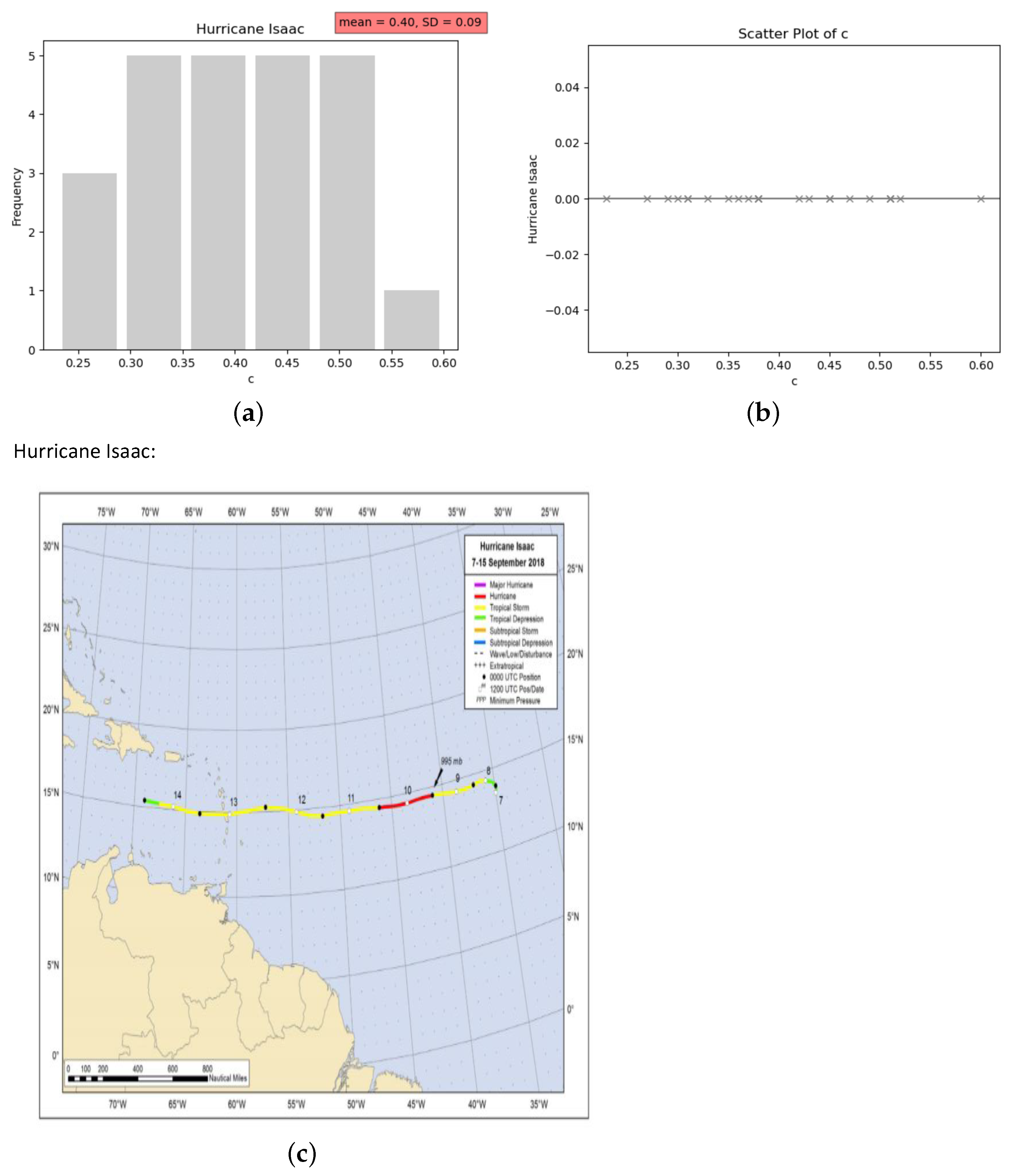
Wind Speed (${\mathit{U}}_0$) (m/s)	Wave Height (H) (m)	c	Details
5.3	1.4	0.49
5.5	1.6	0.52	Station: 41041
5.3	1.45	0.51
5.5	1.32	0.43
5.8	1.54	0.45	Date analyzed: 9 September 2018
6.8	1.45	0.31
6	1.34	0.37
5.6	1.51	0.47	Description: East of Martinique
5.1	1.36	0.51
4.8	1.4	0.6
5.8	1.32	0.38	Time scale: 1 h.
5.9	1.28	0.36
5.7	1.4	0.42
5.3	1.45	0.51	Mean of c: 0.40
5.6	1.45	0.45
6.2	1.36	0.35
6	1.4	0.38	mode of c: 0.51
6.7	1.39	0.3
6.8	1.46	0.31
7	1.47	0.29	Standard deviation of c: 0.09
6.7	1.49	0.33
7.1	1.37	0.27
8.1	1.56	0.23
6.2	1.5	0.38

shows the buoy station’s measurement for wind speeds and significant wave heights over 24 h on 9 September 2018. This was the day when hurricane Isaac passed the buoy site. Near the buoy site, Isaac transitioned from tropical storm to hurricane. The standard deviation of the data for c is very small (0.09) in comparison with the mean value (0.4) and mode value (0.51). The mean value should be a good prediction of c. Figure 2a is the frequency plot of the data for c. It is close to a bell shape. Figure 2b is the scatter plot of the data for c. The data do not scatter too much from the mean value.

Figure 3 is about hurricane Chris (6–12 July 2018) [24]. Figure 3c shows the path of hurricane Chris. The mobile buoy location is near the start of the hurricane portion of the path [Figure 3c].

Table 3. Hurricane Chris buoy measurements taken from [5].

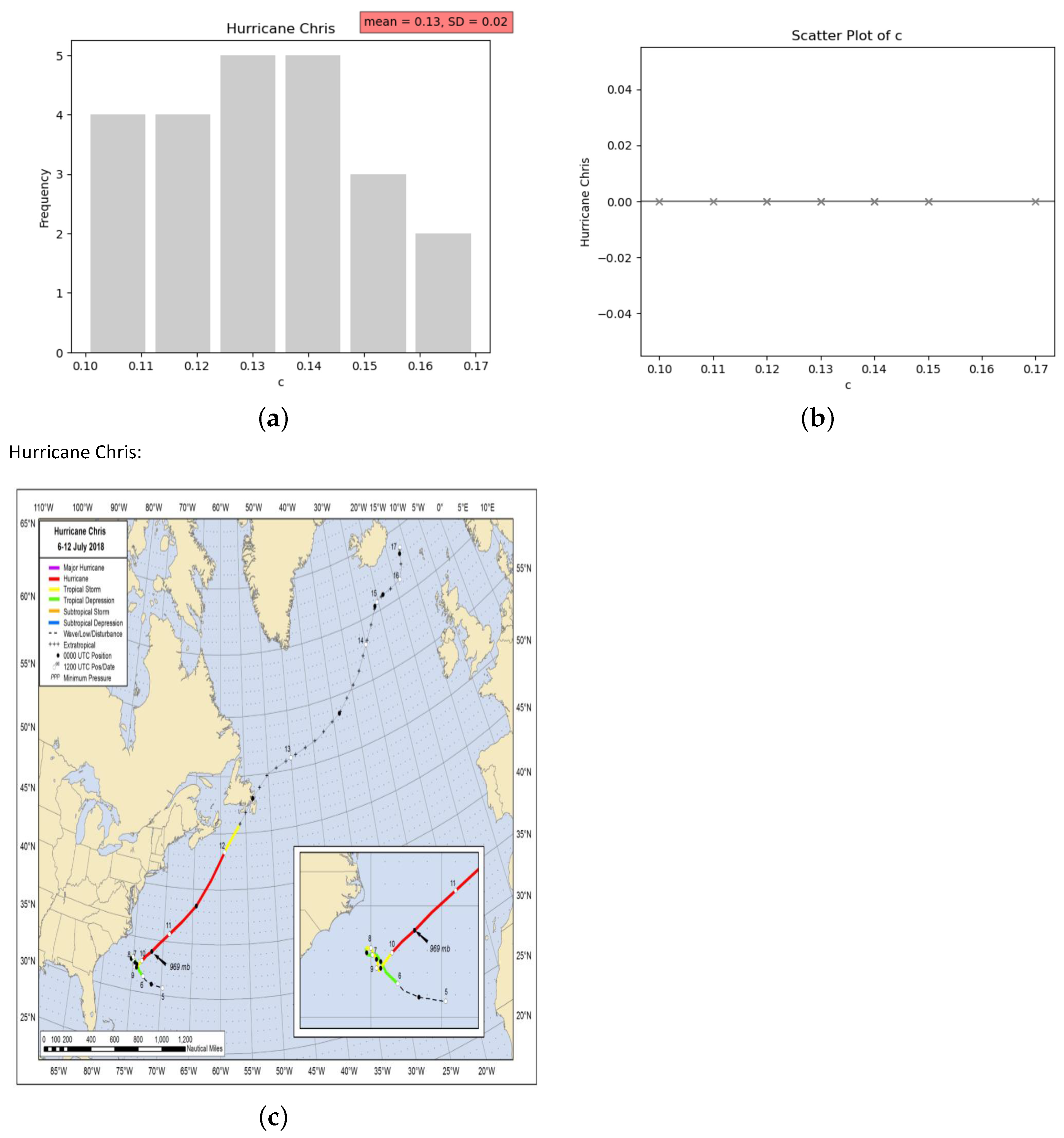
Wind Speed (${\mathit{U}}_0$) (m/s)	Wave Height (H) (m)	c	Details
12.4	2.6	0.17
12.4	2.67	0.17	Station: 41002
13.6	2.47	0.13
13.3	2.6	0.14
12.8	2.53	0.15	Date analyzed: 9 July 2018
14.2	2.72	0.13
13.4	2.8	0.15
15.2	3.09	0.13	Description: South Hatteras
16	3.21	0.12
17.2	3.16	0.1
18.6	3.61	0.1	Time scale: 1 h.
18.2	3.76	0.11
17.1	4.04	0.14
17.3	3.79	0.12	Mean of c: 0.13
15.7	3.42	0.14
15.5	3.28	0.13
16.5	3.5	0.13	Mode of c: 0.13
16.8	3.37	0.12
16.8	3.58	0.12
15.7	3.63	0.14	Standard deviation of c: 0.02
15.7	3.48	0.14
16.9	3.34	0.11
15.4	3.63	0.15

shows the buoy station’s measurement of the 24 h wind speeds and significant wave heights on 9 July 2018. This was the day when Isaac was a tropical storm close to the buoy site, and on the next day, Isaac turned into a hurricane with its eye passing through the buoy site. The standard deviation of the data for c is very small (0.02) in comparison with the mean value (0.13) and mode value (0.13). The mean value should be a good prediction of c. Figure 3a is the frequency plot of the data for c. It is close to a bell shape. Figure 3b is the scatter plot of the data for c. The data do not scatter too much from the mean value.

Figure 4 is about hurricane Maria (16–30 September 2017) [25]. Figure 4c shows the path of hurricane Maria, whist

Table 4. Hurricane Maria buoy measurements taken from [5].

Wind Speed (${\mathit{U}}_0$) (m/s)	Wave Height (H) (m)	c	Details
25.9	5.03	0.07
25.6	5.6	0.08	Station: 42060
23.1	5.46	0.10
19.1	5.22	0.14
20.4	5.32	0.13	Date analyzed: 19 September 2017
19	5.71	0.16
18.8	5.72	0.16
17.6	5.11	0.16	Description: Guadeloupe
16.1	5.44	0.21
14.7	5.13	0.23
14.7	5.03	0.23	Time scale: 1 h.
14	4.72	0.24
13.5	4.36	0.23
12	4.35	0.30	Mean of c: 0.22
13.8	4.44	0.23
15	4.1	0.18
13.3	4.03	0.22	Mode of c: 0.07
13.3	4.3	0.24
10.7	4.33	0.37
11.5	4.08	0.30	Standard deviation of c: 0.08
10.6	3.53	0.31
10.7	3.69	0.32
11.3	3.23	0.25
11.9	3.56	0.25
10.5	3.23	0.29

shows the 24 h wind speed and significant wave heights on 19 September 2017. The standard deviation of the data for c is very small (0.08) in comparison with the mean value (0.22). The mean value should be a good prediction of c. Figure 4a is the frequency plot of the data for c. It is close to a bell shape. Figure 4b is the scatter plot of the data for c. The data do not scatter too much from the mean value.

The mean values of c for hurricanes Florence and Isaac are close, while the mean value of c for hurricane Chris is quite different. Hurricanes Florence and Isaac happened around the same time in September 2018, and both buoy sites were far away from the coasts. Hurricane Chris happened in July 2018, and the buoy site was close to the coast.

The frequency distributions of c are classified as bell shape curves for the four tropical cyclones. These can be classified and quantified as a normal distribution, not restricted to the visual representation of the shape of the data, but the criterion that the mean and the mode (as well as median) are of similar values. It can be seen that, the mean if not equal to the mode, are of close numerical value, with the exception of tropical cyclone, Maria.

Thus, we have the four sample cases displaying normal distributions with relatively small standard deviation values when compared to their mean c values. We can then deduce that the mean values provide good predictions for c. Hence, a significance of this methodology is that relation can be utilized to directly use the c parameter to increase the temporal resolution which would thereafter improve the modeling of these natural phenomena.

3.2. Wind Speed Relation in Comparison to Model Runs

In a study by [26], for hurricane Florence, the relative accuracy of the Hurricane Weather Research and Forecasting (HWRF) model and another model, parametric in nature, referred to as the Holland 2010 wind model (H10), is determined. Using the pressure fields and wind variables determined from these two models, the simulated water level was analyzed using a two-dimensional coastal hydrodynamic model, Delft3D. Two validation locations were compared to in situ observations in the track of hurricane Florence: COOPS and USGS stations. It was determined that, for both stations, the root mean square error (RMSE) for the water level was lower for the HWRF model. For the period of 11–18 September 2018, at the COOPS station, the RMSE for the HWRF and H10 was 0.46 and 0.63 m. Also, for a similar period, 12–18 September 2018, at the USGS station, the hourly water level validation statistics showed that there weer 0.21 and 0.40m RMSEs for HWRF and H10. The max surges driven by both models’ outputs into Delft3D show less error with an approximate error of 0.20 m.

The errors in the simulated wind fields leads to errors in the storm surge simulations. The relation in this paper provides a direct prediction of wave height or wind speeds, given the average c value if the standard deviation is small in comparison to the mean. This methodology also serves as a way to increase the temporal resolution through interpolation once c is determined. This is particularly important as it is predicted that inundation from large storms, over the next century along the coast of the United States, will increase. As shown in the analysis of [27], especially in shallow waters, the overall wave models underestimate the significant wave heights, in the vicinity of the tropical cyclone’s peak, and they display complex wave height bias patterns likely due to the insufficient resolution and errors with the wind inputs. Comparing with buoy 41047, which we examined in our analysis, it was determined by [27] that for hindcasts, the National Centers for Environmental Prediction (NCEP-WW3), the European Center for Medium-Range Weather Forecasts (ECMWF-ERA5), the French Research Institute for the Exploitation of the Sea (IFREMER-WW3) and the U.S. Army Corps of Engineers (USACE-WIS), the significant wave heights were overestimated to an approximate 20–30%, with the exception of ECMWF-ERA5.

4. Conclusions

The relation between wind speed and the maximum or mean wave height that it can generate is studied from the perspectives of mathematics and application.

Dimensional analysis shows that the relation between wind speed and maximum or mean water wave height takes the form $H=c{\displaystyle \frac{U_0^2}{g}}$, where H is the maximum or mean water wave height caused by wind of speed $U_0$, g is the gravitational acceleration, and c is a dimensionless constant. We also use simple mathematical models to study this relation.

We applied the relationship to four hurricanes in terms of significant wave heights rather than overall maximum or mean wave height. The observed values of c are analyzed statistically. On the days when the fixed buoy captured the highest wind speeds, the frequency distributions of the data for c are close to a bell shape with very small standard deviations in comparison with the mean values; thus, the mean values provide good predictions for c. In view of the fact that hurricane waves are turbulent and the background waves caused by many other factors such as lunar tidal effect cannot be ignored, the obtained results for c are quite satisfactory.

For hurricanes Florence and Isaac, which occurred around the same time in September 2018, with both buoy sites far away form the coasts, their mean values for c are close. For hurricane Chris, which occurred in July 2018, with the buoy site close to the coast, its mean value for c is quite different.

Thus, for randomly selected tropical cyclones, the days where the buoys captured the highest wind speed were used in the analysis. Complexities in this study include the turbulent nature of the hurricane waves as well as background waves which may contribute to the variability in the c values for a hurricane system. Future work, given that, mathematically, the dimensional analysis shows the relationship, will be performed to apply this relation to more randomly selected hurricane systems. After this, interpolation of the data can be performed to see any improvements in the modeling of these complex atmospheric phenomena.

Since the wind speeds are above 4 m/s, another future analysis includes the investigation of the power law relation, other than the conventional purely quadratic relation studied here. Such a relation is exemplified in [28] which takes into consideration the average swell.

References

- Park, G. A comprehensive analysis of hurricane damage across the US gulf and atlantic coasts using geospatial big data. ISPRS Int. J. Geo-Inf. 2021, 10, 781. [Google Scholar] [CrossRef]
- Lin, N.; Emanuel, K.A.; Smith, J.A.; Vanmarcke, E. Risk assessment of hurricane storm surge for New York City. J. Geophys. Res. Atmos. 2010, 115, D18121. [Google Scholar] [CrossRef]
- Lin, N.; Emanuel, K.; Oppenheimer, M.; Vanmarcke, E. Physically based assessment of hurricane surge threat under climate change. Nat. Clim. Chang. 2012, 2, 462–467. [Google Scholar] [CrossRef]
- Knauss, J.A.; Garfield, N. Introduction to Physical Oceanography; Waveland Press: Long Grove, IL, USA, 2017. [Google Scholar]
- National Data Buoy Center; National Oceanic and Atmospheric Administration. National Data Buoy Center. 2024. Available online: https://www.ndbc.noaa.gov/ (accessed on 20 January 2020).
- Katalinić, M.; Ćorak, M.; Parunov, J. Analysis of wave heights and wind speeds in the Adriatic Sea. Marit. Technol. Eng. 2014, 1, 1389–1394. [Google Scholar]
- Kumar, V.S.; Mandal, S.; Kumar, K.A. Estimation of wind speed and wave height during cyclones. Ocean. Eng. 2003, 30, 2239–2253. [Google Scholar] [CrossRef]
- Phadke, A.C.; Martino, C.D.; Cheung, K.F.; Houston, S.H. Modeling of tropical cyclone winds and waves for emergency management. Ocean. Eng. 2003, 30, 553–578. [Google Scholar] [CrossRef]
- Drazin, P.G.; Reid, W.H. Hydrodynamic Stability, 2nd ed.; Cambridge Mathematical Library, Cambridge University Press: Cambridge, UK, 2004; pp. xx+605. [Google Scholar] [CrossRef]
- Miles, J.W. On the generation of surface waves by shear flows. J. Fluid Mech. 1957, 3, 185–204. [Google Scholar] [CrossRef]
- Miles, J.W. On the generation of surface waves by shear flows. II. J. Fluid Mech. 1959, 6, 568–582. [Google Scholar] [CrossRef]
- Miles, J.W. On the generation of surface waves by shear flows. III. Kelvin-Helmholtz instability. J. Fluid Mech. 1959, 6, 583–598. [Google Scholar] [CrossRef]
- Janssen, P. The Interaction of Ocean Waves and Wind; Cambridge University Press: Cambridge, UK, 2004. [Google Scholar]
- Lokharu, E.; Wahlén, E.; Weber, J. On the amplitude of steady water waves with favorable constant vorticity. J. Math. Fluid Mech. 2023, 25, 7. [Google Scholar] [CrossRef]
- Lokharu, E. A sharp version of the Benjamin and Lighthill conjecture for steady waves with vorticity. arXiv 2020, arXiv:2011.14605. [Google Scholar] [CrossRef]
- Benjamin, T.B.; Lighthill, M.J. On cnoidal waves and bores. Proc. R. Soc. Lond. Ser. Math. Phys. Sci. 1954, 224, 448–460. [Google Scholar]
- Benjamin, T.B. Verification of the Benjamin–Lighthill conjecture about steady water waves. J. Fluid Mech. 1995, 295, 337–356. [Google Scholar] [CrossRef]
- Kozlov, V.; Kuznetsov, N. The Benjamin–Lighthill conjecture for near-critical values of Bernoulli’s constant. Arch. Ration. Mech. Anal. 2010, 197, 433–488. [Google Scholar] [CrossRef]
- Balkissoon, S.S.; Bongard, J.T.; Cain, T.; Candela, D.M.; Clay, C.; Efe, B.; Ji, Q.; Klaus, E.M.; Korner, A.P.; Mitchell, K.; et al. Hurricane florence makes landfall in the Southeast USA: Sensitive dependence on initial conditions, parameterizations, and integrated enstrophy. Atmos. Clim. Sci. 2020, 10, 101–124. [Google Scholar] [CrossRef]
- Stewart, S.R.; Berg, R.N.H.C. National Hurricane Center Tropical Cyclone Report, Hurricane Florence. 2019. Available online: https://www.nhc.noaa.gov/data/tcr/AL062018_Florence.pdf (accessed on 15 July 2021).
- Young, I. Seasonal variability of the global ocean wind and wave climate. Int. J. Climatol. J. R. Meteorol. Soc. 1999, 19, 931–950. [Google Scholar] [CrossRef]
- Ribal, A.; Young, I.R. 33 years of globally calibrated wave height and wind speed data based on altimeter observations. Sci. Data 2019, 6, 77. [Google Scholar] [CrossRef] [PubMed]
- Zelinsky, D.A. National Hurricane Center Tropical Cyclone Report, Hurricane Isaac. 2019. Available online: https://www.nhc.noaa.gov/data/tcr/AL092018_Isaac.pdf (accessed on 18 September 2021).
- Blake, E.S. National Hurricane Center Tropical Cyclone Report, Hurricane Chris. 2018. Available online: https://www.nhc.noaa.gov/data/tcr/AL032018_Chris.pdf (accessed on 5 December 2021).
- Pasch, R.J.; Penny, A.B.; Berg, R.N.H.C. National Hurricane Center Tropical Cyclone Report, Hurricane Maria. 2023. Available online: https://www.nhc.noaa.gov/data/tcr/AL152017_Maria.pdf (accessed on 22 January 2023).
- Rahman, M.A.; Zhang, Y.; Lu, L.; Moghimi, S.; Hu, K.; Abdolali, A. Relative accuracy of HWRF reanalysis and a parametric wind model during the landfall of Hurricane Florence and the impacts on storm surge simulations. Nat. Hazards 2023, 116, 869–904. [Google Scholar] [CrossRef]
- Rogowski, P.; Merrifield, S.; Collins, C.; Hesser, T.; Ho, A.; Bucciarelli, R.; Behrens, J.; Terrill, E. Performance assessments of hurricane wave hindcasts. J. Mar. Sci. Eng. 2021, 9, 690. [Google Scholar] [CrossRef]
- Gao, Y.; Schmitt, F.G.; Hu, J.; Huang, Y. Probability-based wind-wave relation. Front. Mar. Sci. 2023, 9, 1085340. [Google Scholar] [CrossRef]