High-Resolution WRF Modeling of Wind and Thermal Regimes with LCZ in Almaty, Kazakhstan

Abstract

This study evaluates the effectiveness of the Weather Research and Forecasting (WRF) model in simulating high-resolution atmospheric conditions for Almaty, Kazakhstan, a city prone to stagnant winter air. While the previously used Bougeault and Lacarrere scheme for parameterizing the planetary boundary layer was applied in high-resolution modeling, the number of vertical levels was increased, and a detailed local climate zones (LCZs) map was included. Ground-based observations from meteorological stations and monitoring stations, remote sensing data, and radiosonde measurements are used to verify the model. Comparison results with ground-based observations show that the WRF model with the LCZ map provides a better representation of the wind and thermal regimes of Almaty compared to the three-class land use map, including in high resolution. A good correspondence of wind direction is demonstrated by comparing the modeling results with pollutant transport plumes recorded by remote sensing data. In addition, a good correlation was found between land surface temperature from satellite data and air temperature simulated by WRF with a resolution of 333 m. A comparison of simulated data and aerological measurements confirmed that downscaling did not have a significant impact on boundary layer calculations. Analysis of turbulent processes showed that the adopted model effectively describes the attenuation and dissipation of turbulent kinetic energy and reflects the typical diurnal variations of meteorological processes in the atmosphere of Almaty in the anticyclonic winter period. The results of high-resolution WRF modeling can form the basis for the development of a hybrid system capable of modeling atmospheric processes at the building level.

1. Introduction

Almaty, the largest city in Kazakhstan, sits in a wind shadow at the foot of the Tien Shan mountains. This geographical location leads to frequent calms, light winds, and temperature inversions, which result in high levels of air pollution. The urban development hinders the already weak wind to an almost complete state of windlessness. It is worth noting that the city is built chaotically. Multi-story buildings go up close to five- to nine-story buildings on a small island, closely adjacent to each other.

Considering this, there is a pressing need to analyze wind and thermal regimes to develop an appropriate strategy for further urban development while keeping optimal ventilation. Such an analysis can be performed by integrating meso- and microscale models, which will make it possible to tackle environmental problems in Almaty fully, considering its multi-level processes.

This study builds on earlier work by the authors to adapt the Weather Research and Forecasting (WRF) [1] model with a maximum resolution of 1 km to the complex conditions of Almaty [2,3]. To effectively integrate the results of mesoscale modeling into a microscale model, the resolution of the WRF model needs to be increased [4,5].

Advances in computer processing power have made it possible to perform WRF modeling at high spatial resolutions. In work [6], WRF modeling was successfully applied to study turbulence and the evolution of the atmospheric boundary layer with horizontal resolutions of 2700, 900, 300, and 100 m. The study in [7] examined how water bodies affect the urban thermal environment using WRF modeling with nested domains of 4.5 km, 1.5 km, and 500 m. Applying WRF modeling [8] for short-term and medium-term precipitation forecasting in complex orographic conditions (central Andes, Peru) demonstrated an effective simulation of accumulated precipitation in the 3 km resolution domain, with better reproduction of the process in the 0.75 km grid spacing domain at the local scale.

This study aims to analyze the results of WRF modeling with a resolution of 333 m for Almaty City for further use in microscale modeling of wind circulation and other meteorological processes.

Unfortunately, increasing the resolution to 333 m pushes the modeling physics into the so-called “gray zone” where neither traditional mesoscale model using planetary boundary layer (PBL) parameterization nor large eddy simulation (LES) are fully applicable [6,9]. This study employs the Bougeault and Lacarrere (BouLac) PBL scheme [10], a choice motivated by its superior performance in previous studies [2,3] with a maximum resolution of 1 km. The choice of this PBL scheme is dictated using the Building Environment Parametrization (BEP) [11] for building effects. To mitigate the “gray zone” effect, this study (1) refined the underlying urban surface data and (2) increased the number of vertical levels, including reducing the vertical spacing to 4 m in the lowest layer (building layer) [12]. The results are compared against all available measurement data to validate the model’s performance with the chosen parameterization configuration.

Input data such as topography and land use maps created with a higher level of detail can effectively improve the numerical modeling of meteorological parameters. Specifically, in the study [13], the authors evaluated the impact of land use and land cover on the results of WRF modeling with resolutions of 500 m and 100 m. The study [14] showed that land use data significantly influences the results of the WRF model in mountainous terrain, and a fine grid spacing (500 m) allows more accurate modeling of diurnal mountain wind patterns.

When using the WRF model for urban areas, the underlying urban surface data are used as a land use map. This study analyzes the use of local climate zones (LCZs) classification instead of the three urban land use classes previously used by authors.

Canadian geographers Stewart and Oke [15] developed the concept of LCZs in response to the pressing need for more standardized research on urban climates. This concept aims to define morphological types of the urban surface considering local climate conditions. Field studies validated the LCZ concept based on the experience of previous classifications. Subsequently, the World Urban Database and Access Portal Tools (WUDAPT) project was created to collect and disseminate information about urban and rural surfaces [16]. The authors [17] reviewed 91 studies focusing on the problems of mapping LCZs in Europe. This study concludes that the LCZ classification has established itself as a versatile method for describing the urban environment. The key property of LCZs is that local climate zones within urban development are defined by a combination of urban morphology factors and the thermal properties of buildings, which makes it an important basis for studying urban climate [15].

WRF researchers have also successfully applied LCZ classification as land use input data. For example, researchers in [18,19,20] have demonstrated that LCZ data can improve WRF weather modeling results. They showed that the BEP parameterization is sensitive to landscape heterogeneity. The use of LCZ data has proven successful in modeling the temperature regime of urban areas in Szeged, Hungary [21]. Mu et al. positively evaluated the use of LCZ classification for mesoscale modeling of a megacity like Beijing [22]. McRae et al. [23] included LCZs in WRF boundary condition modeling for ENVI-met for San Jose, California. Richard et al. [24] considered the significance of LCZs in modeling temperature regimes using the example of the city of Dijon, France. Du et al. [25] studied the impact of LCZ classification combined with a building category map on WRF modeling of urban climate and air conditioning load in Hong Kong. WUDAPT LCZ classification [26] resulted in more realistic and consistent simulations of heavy rainfall events in Bangalore, India (2020–2022) within the WRF modeling framework.

Section 2 of this paper is dedicated to the research methodology, including a description of the underlying surface used, the configuration of nested domains with the inclusion of a new domain (D4) with a resolution of 333 m in the downscaling procedure, methods of parametrizing microphysical processes that adapt WRF to the conditions of Almaty city, as well as methods of analyzing the results obtained. Section 3 is dedicated to the analysis of the results obtained. Verification of the modeling results employed all available field observations, including measurements of temperature and wind from weather stations and sensors, radiosonde data, and visible and thermal satellite imagery. A comparison of the modeling results using three classes of urbanized territories and LCZs with 10 urban classes with data of field measurements at weather stations is presented, as well as the average (BIAS), absolute (MAE), and root mean square (RMSE) errors are shown (Section 3.1). Verification of the modeling results of the spread of emissions from large thermal power plants using the System for Integrated Modeling of Atmospheric Composition (SILAM) [27] model with remote sensing data in the visible range (Landsat 8–9) [28] was carried out (Section 3.2). Such an analysis makes it possible to judge the adequacy of wind regime modeling in WRF. A comparison of the modeling results of D3 (1 km) and D4 (333 m) domains with field measurements of meteorological parameters was carried out (Section 3.3). A comparison of the modeling results of the thermal regime of the city of Almaty with a resolution of 333 m with data of remote sensing in the thermal range from Landsat 8–9 satellites was carried out (Section 3.4). A joint analysis of the modeling results with data from aerological observations for domains with a resolution of 1 km and 333 m was also carried out (Section 3.5). Section 3.6 evaluates the adequacy of the 333 m resolution modeling results in capturing turbulent processes.

2. Materials and Methods

2.1. Description of the Object under Study

Almaty is the largest city in Kazakhstan, located in the southeastern part of the country (43°15′ N 76°54′ E). As of 1 May 2024, the metropolis is home to more than 2.2 million people [29]. The city covers a total area of 680 sq km, with approximately 52% constituting the built-up area located in the northern part. Due to its unique location in the shadow of the Zailiyskiy Alatau mountain range, Almaty is characterized by a high frequency of calm conditions, especially in winter—79% [30]. The situation is exacerbated by a temperature inversion layer that blocks vertical exchange. Such unfavorable meteorological conditions are formed in winter, mainly due to the influence of the Asian (Siberian) anticyclone [31].

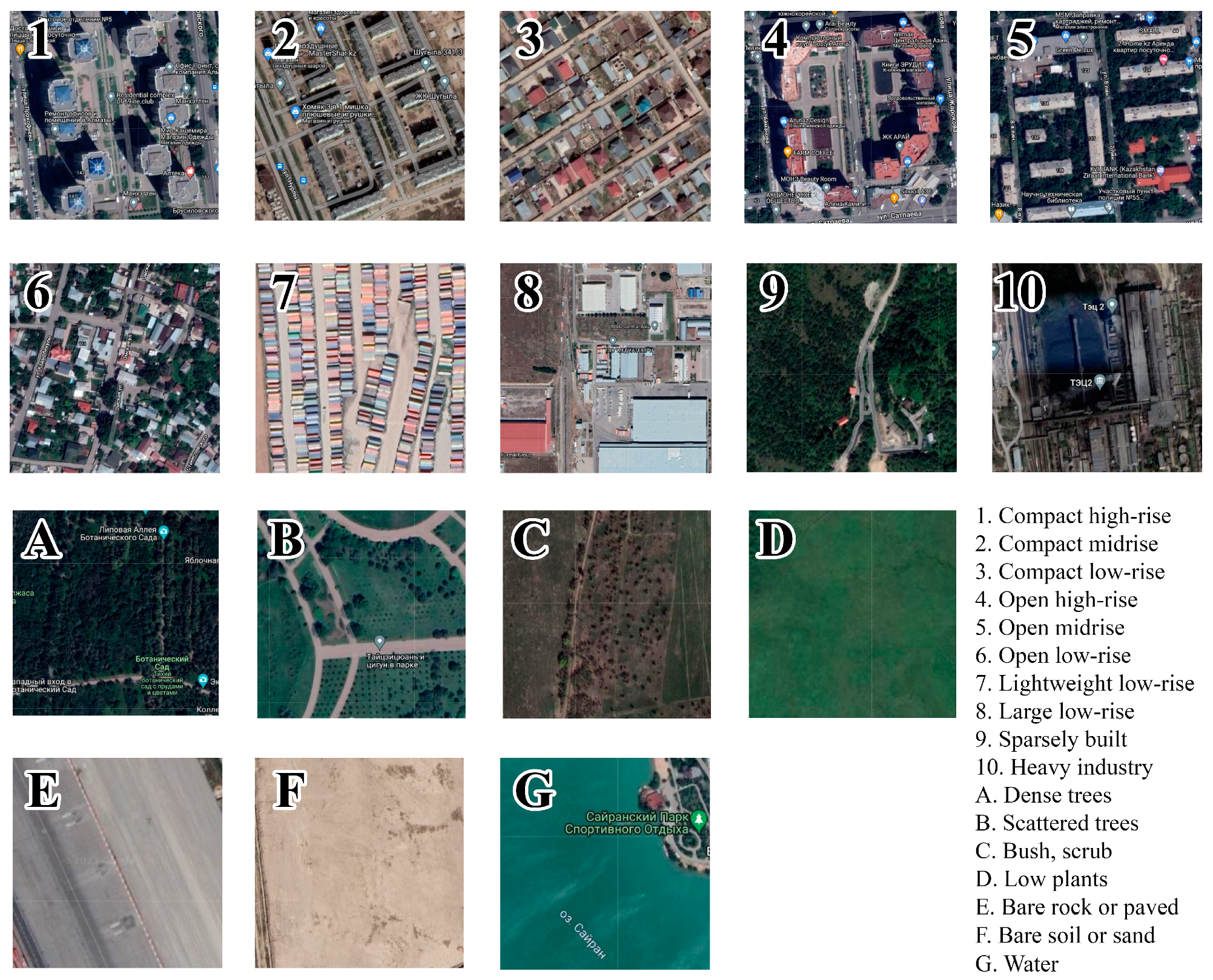
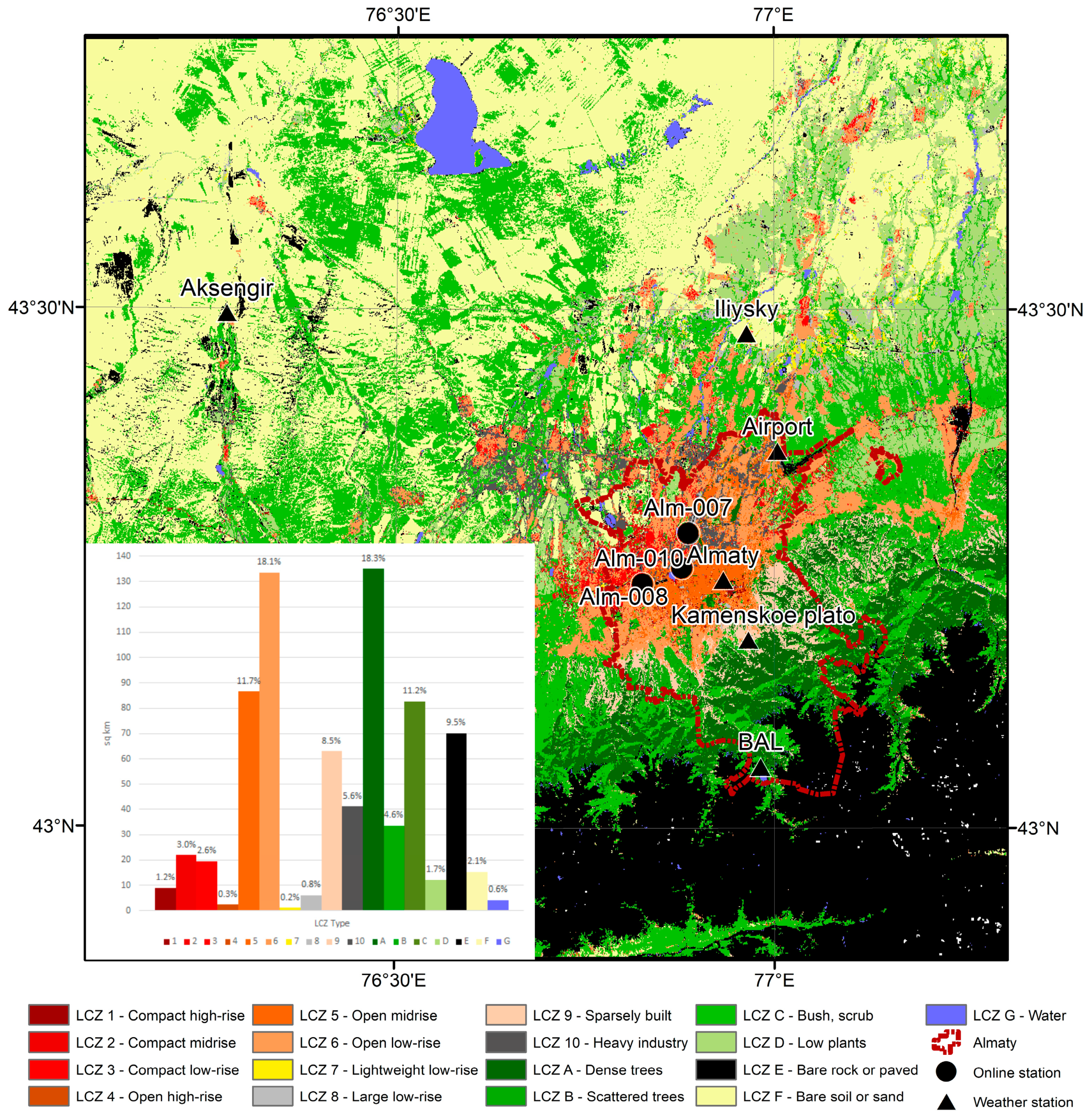
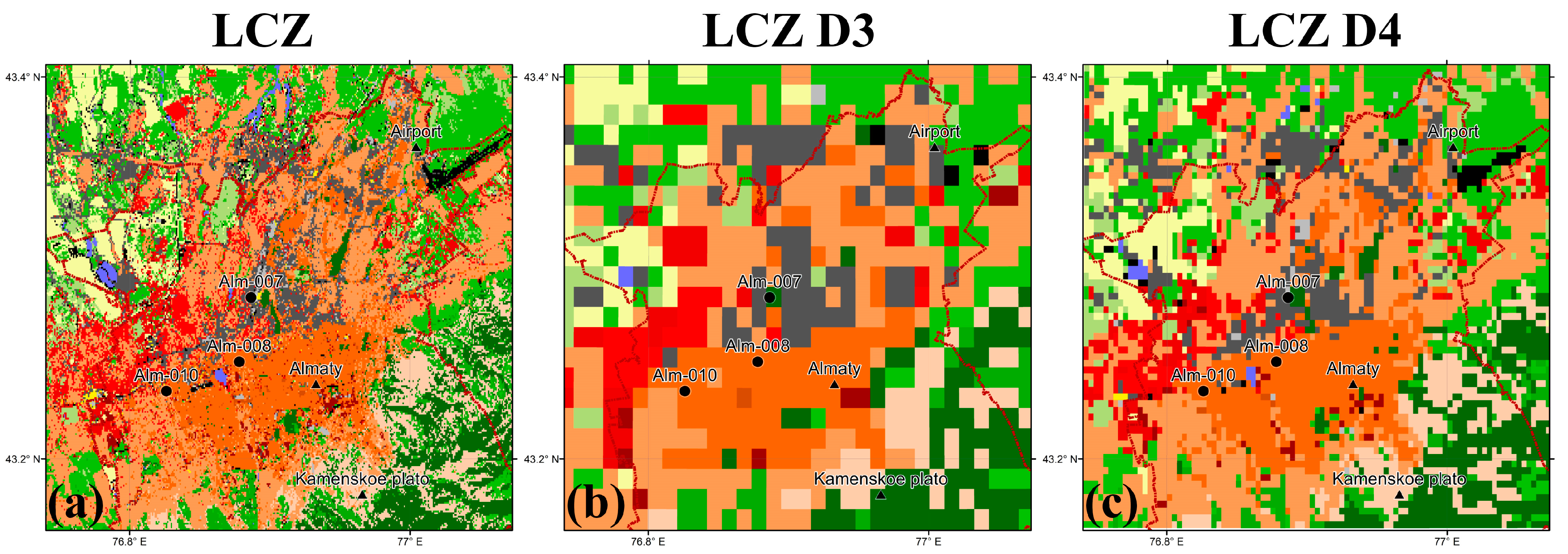
2.2. Land Use/Land Cover

Within the framework of this study, a land use map was developed for the city of Almaty as input data on the underlying surface. The map represents the local climate zones, where instead of three urban classes used by authors earlier [2,3], 10 urban classes (LCZ 1–LCZ 10) and seven types of local zones of natural territories (LCZ A–LCZ G) are considered.

The map of local climate zones for the city of Almaty was obtained using the LCZ Generator tool [32]. This online tool [33] maps LCZs based on training polygons and subsequent training with the identification of suspicious areas. Examples of territories corresponding to different types of LCZs for the city of Almaty are presented below (Figure 1).

This tool provides an automatic assessment of the accuracy of the mapping performed. The resulting map of local climatic zones for the city of Almaty is characterized by an average overall accuracy (OA—54%) and average accuracy for urban classes (OA_u—52%), high weighted accuracy OA_w—87%, and the accuracy of distinguishing urban development zones (LCZ 1–LCZ 10) from natural zones (LCZ A–LCZ F)—OA_bu was 88%, which is important for taking into account the boundaries of urbanization in WRF modeling. The spatial resolution of the resulting map is 90 m. Figure 2 illustrates the constructed map of local climate zones for Almaty and its environs.

An analysis of the distribution of the obtained local climate zones within the Almaty city border showed that the most common zone is the open low-rise development zone (LCZ 6)—18.1%, which corresponds to the private sector, summer cottage settlements, and gardening associations. The second largest area is open medium-rise development (LCZ 5), typical of residential areas—11.7%. In third place is the sparse low-rise development zone (LCZ 9), occupying 8.5% of the total area of the city. All urban classes occupy 52.1% and are located in the northern part of the city. Among the natural zones in Almaty, the dense forest zone (LCZ A) dominates and is widespread in the foothills. In general, four “green” natural zones occupy about 35.8% of the city’s territory, while the remaining 12.1% are natural areas devoid of vegetation. These are rocks, stones, and water bodies (Figure 2).

2.3. WRF Model Domain

The LCZ map for Almaty provides a more precise characterization of the underlying surface, paving the way for a more detailed mesoscale WRF model. For this purpose, four domains in Lambert conformal conic projection were created for Almaty in WRF modeling [1] instead of the three used in earlier studies [2,3]. The first domain (D1) has a grid cell size of 9 km, the second domain (D2) has a grid cell size of 3 km, the third domain (D3) has a grid cell size of 1 km, and the fourth domain (D4), focused on the built-up area of the city, has a grid cell size of 333 m. The first three domains contain 100 grid cells from west to east and 100 grid cells from south to north, while the fourth domain has 82 by 82 grid cells. Time steps for simulations within D1, D2, D3, and D4 are 18, 6, 2, and 2/3 s, respectively. Vertically, 45 levels are employed, with a 4 m step in the lowest layer (building layer) to utilize a multi-layer model that incorporates Building Environment Parameterization (BEP) [11]. The overall configuration of the nested domains is illustrated in Figure 3.

2.4. Model Configuration and Simulations

ASTER GDEM (Global Digital Elevation Model) [34] data with a spatial resolution of 1 arc second (approximately 30 m) were used as the terrain data. The Global Forecast System (GFS) from the National Centers for Environmental Prediction (NCEP) [35] provided the initial and boundary conditions for the simulations. These conditions have a spatial resolution of 0.25 degrees by 0.25 degrees and a time step of 3 h.

All calculations were performed for the period from 13 to 23 January 2023, when an unfavorable synoptic situation, “Asian anticyclone ridge”, persisted, which is characteristic of the city of Almaty in the winter season.

The optimal configuration of parameterization methods was selected by the authors in the previous stages of the work [2,3]. It is based on a large series of test calculations and the experience of other scientists who apply the WRF model to cities located in complex mountainous terrain [36,37,38,39]. In this work, this configuration remained unchanged.

Table 1. Details of the WRF model configuration and experiments.

Parameters/Experiments	WRF LCZ (WRF D3)	WRF D4	WRF Urban3
Domain grid cell size (km)	1	0.333	1
Initial and boundary conditions	D2 (two-way nested)	D3 (two-way nested)	D2 (two-way nested)
Simulated period	From 00:00 GMT 13 January 2023 to 00:00 GMT 23 January 2023
Microphysics	WRF Single-Moment 6-Class Microphysics Scheme (WSM6) [40]
PBL Physics	Bougeault and Lacarrere parameterization (BouLac) [10]
Convection	Kain–Fritsch parameterization (KF) [41]
Radiation	Rapid Radiative Transfer Model for General circulation models (RRTMG) [42]
Turbulence	2D Smagorinsky parameterization [1].
Surface layer	Monin–Obukhov (Janjic) scheme (MO) [43]
Land/urban surface	Unified Noah land surface model [44]/BEP parameterization [11]
Land use	LCZ	LCZ	USGS +3 urban classes

details the experiments and parameterization methods used.

2.5. Methodology for Comparing Simulations with Observations

First, within the third domain, the modeling results using the land use map for 3 urbanized classes were compared with the modeling results using LCZs. The obtained modeling results were compared with ground-based observations of six meteorological stations of the Kazhydromet network (National Hydrometeorological Service of Kazakhstan)—Almaty, Airport, Iliysky and Kamenskoe Plato, Aksengir, and Big Almaty Lake (BAL). Meteorological observations at an 8-time-per-day frequency are available in the “Weather in 241 countries of the world” database [45]. The accuracy of temperature measurements at weather stations is 0.1 °C (1 °C for the Airport weather station), 1 m/s for wind speed, and one compass point (22.5°) for wind direction. The location of the meteorological stations is illustrated in Figure 3. During the comparative analysis, the first day of calculations was not considered, as it was allocated for model spin-up.

Data from all these meteorological stations were used to evaluate the errors in temperature, wind speed, and wind direction. The following statistical characteristics were calculated for this purpose [46]:

$$BIAS={\displaystyle \frac{1}{n}}{{\displaystyle \sum }}_{i=1}^n\left({\overline{X}}_i-{\widehat{X}}_i\right),$$

$$MAE={\displaystyle \frac{1}{n}}{{\displaystyle \sum }}_{i=1}^n\left|\left({\overline{X}}_i-{\widehat{X}}_i\right)\right|,$$

$$RMSE=\sqrt{{\displaystyle \frac{1}{n}}{{\displaystyle \sum }}_{i=1}^n{\left({\overline{X}}_i-{\widehat{X}}_i\right)}^2}$$

Here, ${\overline{X}}_i$ represents the calculated value at the i-th moment in time, while ${\widehat{X}}_i$ denotes observations from weather stations at the i-th moment in time. The variable n denotes the total number of measurements from weather stations at various time points.

Due to the limited network of meteorological observations, especially in the built-up area of the city of Almaty, it is challenging to conduct a thorough analysis of the obtained modeling results. Therefore, remote sensing data from Landsat 8–9 satellites in the visible and thermal ranges were used for comparison [28]. Such comparisons are used by researchers to evaluate modeling results [47,48,49].

To verify the adequacy of WRF wind field simulations, the results of air pollution calculations were compared with data from Landsat 8–9 satellites in the visible range, which show the plume of pollutants emitted from large thermal power plants. For this purpose, the SILAM model (System for Integrated Modeling of Atmospheric Composition) [27] was used in this work to calculate air pollution, which is widely used to assess air quality and predict the spread of pollutants [50,51,52]. The results of WRF modeling with a spatial resolution of 1 km were used as input meteorological data for the SILAM model. Sulfur dioxide (SO₂) was chosen as the pollutant from CHP-2 and CHP-3 (combined heat and power plants) sources.

Table 2. Sources of emissions.

Name	Lat	Lon	Source Height, m	Source Power, kg/h
CHP-2	43.29	76.797	129	3275.6
CHP-3	43.42	77.01	60	1156.4

shows the main characteristics of the pollution sources used in the modeling and taken from the data on the inventory of stationary sources of current maximum permissible emission projects.

With the increase in the model resolution to 333 m and the addition of the fourth domain, a more detailed comparison of modeling results in different domains with in situ measurements became necessary. Within the built-up area of the city, within the fourth domain, Kazhydromet has only three meteorological stations: Airport, Almaty, and Kamenskoe Plato. Due to the limited network of meteorological observations, data from AMS-09 series air quality monitoring stations [53] were additionally used for comparison with modeling results, namely Alm-007, Alm-008, and Alm-010. These stations are equipped with modules for measuring air temperature and wind speed in a combined housing. The temporal resolution is 20 min, the accuracy of temperature measurements is 0.1 °C, wind speed is 0.05 m/s, and direction is 0.005°. The installation height of such stations is about 2.5–3 m above the surface and, as a rule, near buildings, which does not correspond to the standards for the placement of meteorological stations and can lead to errors when compared with model data. The location of the stations is shown in Figure 3.

To verify the model’s representation of the thermal regime, remote sensing data in the thermal range from the Landsat-8–9 satellites (Thermal Infrared Sensor—Band 10) [28] with a resolution of 30 m were used. For this purpose, correlation relationships were constructed between the land surface temperature (LST) recorded by remote sensing data and the air temperature in the atmospheric boundary layer at a height of 2 m (T2) calculated in WRF.

In constructing correlation plots, Landsat 8–9 satellite images with an original spatial resolution of 30 m were first generalized to a resolution of 330 m (corresponding to the D4 domain with a step of 333 m) using the Aggregate procedure with the MEAN option. Temperature profiles were also constructed in the south–north and west–east directions through the Almaty meteorological station point.

In addition, a comparison was made between radiosonde data obtained from the aerological station near Almaty airport (lon 77.00, lat 43.36) twice a day at 06:00 and 18:00 local time [54] with the calculated meteorological parameters.

To evaluate the results of modeling turbulent processes, graphs of the power spectral density (PSD) of wind speed by using the Welch method [55] were constructed, and a comparative analysis was conducted for both D3 and D4 domains. Vertical profiles and horizontal cross-sections of turbulent kinetic energy (TKE) are presented.

3. Results and Discussion: Thermal and Wind Regime

3.1. Comparative Analysis for Various Land Use Maps

Comparative analysis of WRF modeling results with meteorological observation data suggests that simulating Almaty’s territory with the LCZ method yields better agreement for two key meteorological parameters: temperature (T) and wind speed (v).

Table 3. Accuracy assessment of experiments for the D3 domain.

Name	Coordinates		BIAS_T, °C		MAE_T, °C		RMSE_T, °C		BIAS_v, m/s		MAE_v, m/s		RMSE_v, m/s
	Lat	Lon	LCZ	Urb3	LCZ	Urb3	LCZ	Urb3	LCZ	Urb3	LCZ	Urb3	LCZ	Urb3
Almaty	43.24	76.93	−0.10	−1.86	0.92	1.88	1.15	2.10	0.11	0.26	0.30	0.39	0.55	0.63
Airport	43.36	77.00	−1.56	−2.55	1.81	2.56	2.28	3.03	−0.47	−0.51	0.96	1.00	1.21	1.25
Kamenskoe Plato	43.18	76.97	0.03	−0.50	0.93	0.94	1.18	1.22	−0.63	−0.05	0.76	0.64	1.01	0.85
BAL	43.06	76.98	0.79	0.85	1.57	1.59	1.99	2.03	0.24	0.45	1.09	0.83	1.45	1.08
Iliysky	43.48	76.96	−1.08	−2.78	1.81	2.81	2.41	3.11	0.15	0.81	0.50	1.26	0.77	1.52
Aksengir	43.50	76.27	0.34	−0.13	1.91	1.51	2.35	1.92	−0.24	0.39	0.67	1.05	0.97	1.36
Mean			0.65	1.44	1.49	1.88	1.89	2.24	0.31	0.41	0.71	0.86	0.99	1.12

summarizes the mean deviations (BIAS), mean absolute error (MAE), root mean square error (RMSE), and overall mean error for all six meteorological stations. As shown in the table, five stations exhibit minimal errors in temperature for temperature when simulated using LCZs. However, the Askengir station shows better results using the three urbanized classes for temperature. This might be due to the generalization of the land use map during the simulation, resulting in this station being assigned to an incorrect local climate zone. Wind analysis reveals that all stations on flat terrain perform better with LCZs. Conversely, stations in complex terrain (Kamenskoe Plateau and BAL) showed better agreement with observational measurements when modeled using three urbanized classes. It is noteworthy that the average correlation indicates slightly lower values for simulations using LCZs.

The figures below provide a detailed comparison of temperature (Figure 4), wind speed (Figure 5), and wind direction (Figure 6) for each meteorological station. Figure 4 reveals that both simulations capture the daily temperature cycle (diurnal variation) but struggle with accurately representing extreme temperatures. Focusing on temperature, the red line (LCZ simulation) shows the best agreement with observations (green line) for most stations. This is particularly evident in urban areas like Almaty and Iliysky, where the land use map transitioned from three classes to LCZs. Improvements are less pronounced at the Airport station (border of Almaty) and the Kamenskoe Plato and BAL stations (foothills and mountains), where the terrain complexity might play a role. Notably, the Aksengir station, which favored the three-class land use map for temperature simulations, does not exhibit significant differences in the temperature comparison plot.

Analysis of wind speed plots (Figure 5) reveals a stronger correlation with observational measurements when the simulation incorporates LCZ data for stations located on flat terrain. However, the wind speed plot for the Kamenskoe Plato station shows a decrease in wind speed compared to observations. Conversely, model data with LCZs for the BAL station exhibits peak wind speed values that significantly exceed observed values.

Observation data are absent from Figure 4 and Figure 5 because of unforeseen issues. This could be caused by errors in data collection or problems sending the information.

Wind roses in Figure 6 reveal discrepancies between wind flow directions simulated by the WRF model and those expected for complex terrain with low wind velocities. These discrepancies occur for both the three-class and LCZ classification approaches used in the simulation. Despite these differences, the WRF model generally captures the dominant wind direction accurately.

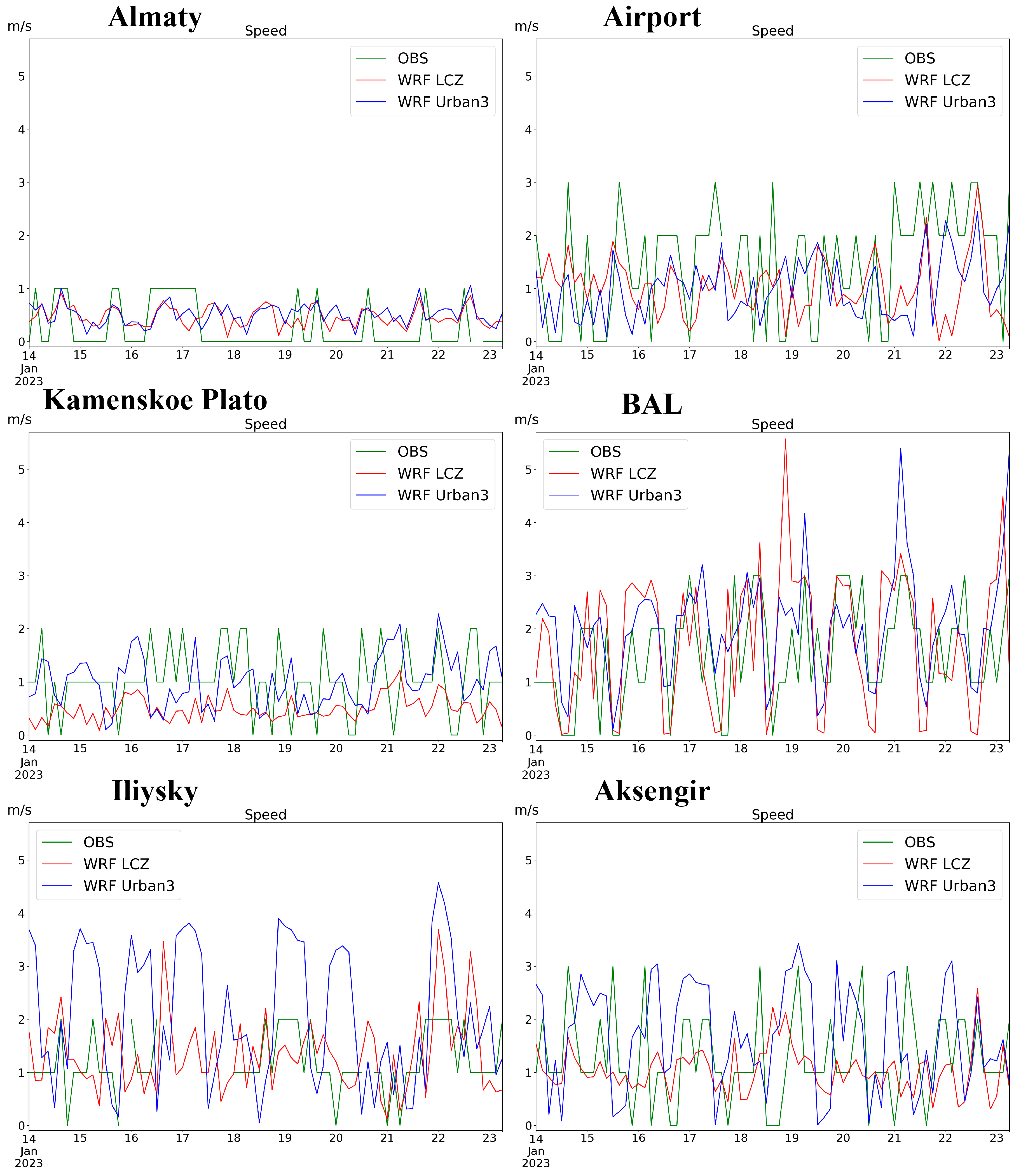
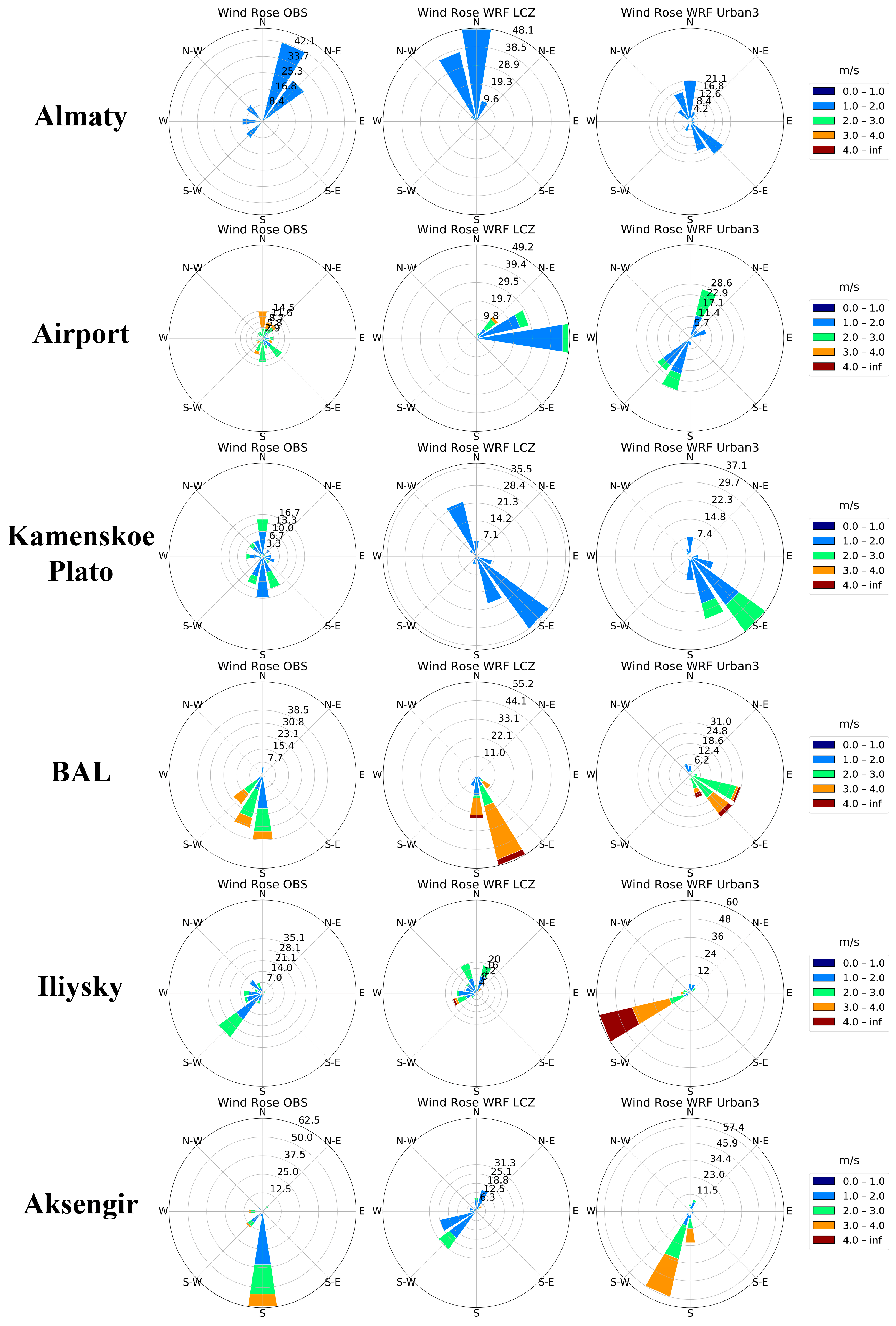
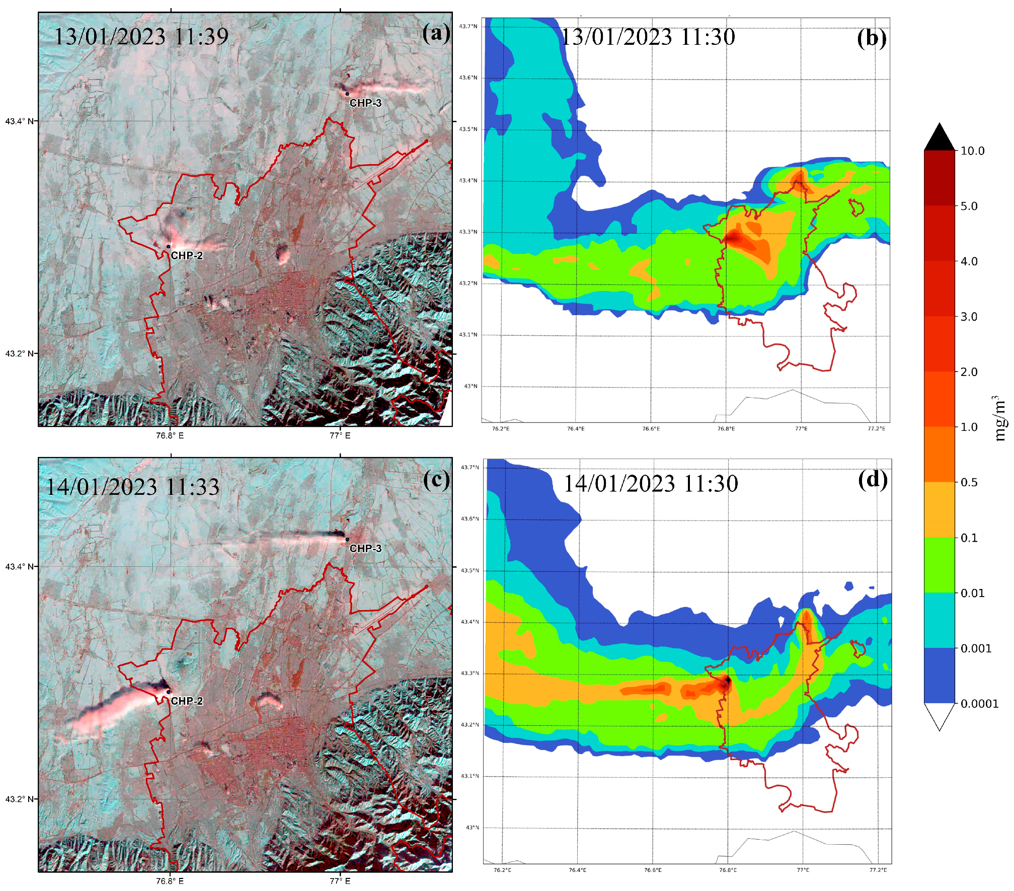
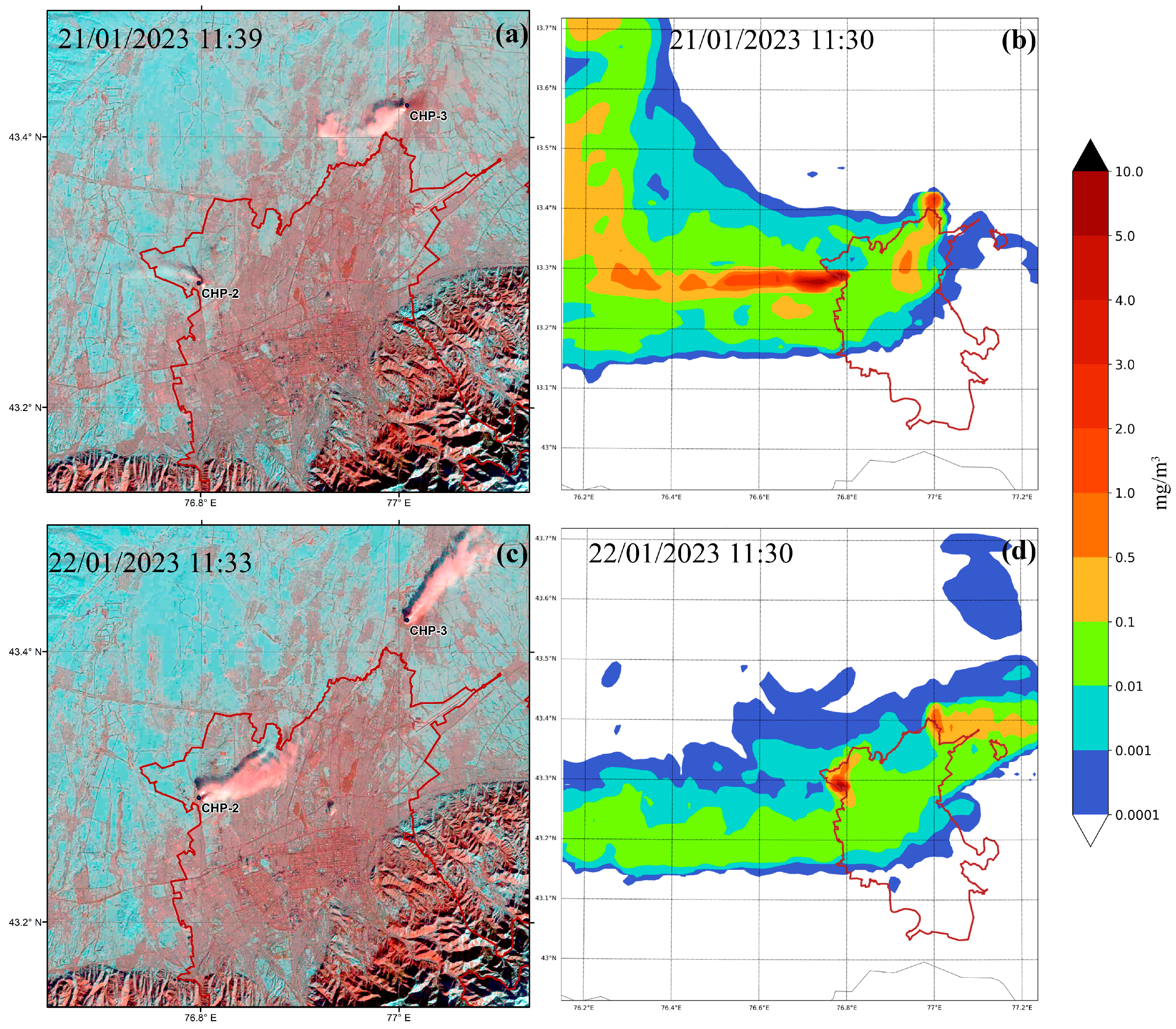
3.2. Comparison of Wind Regime with Remote Sensing Data

Due to the limited availability of meteorological observation network data, an additional analysis of wind regime modeling results was conducted using satellite remote sensing data from Landsat. For this purpose, the SILAM model results were compared with pollutant plume patterns clearly visible in visible-range satellite imagery.

In the figure below (see Figure 7a,c), the Landsat 8–9 space images in the visible range and the simulation results of the SILAM model (see Figure 7b,d) for 13 and 14 January 2023 are presented. Two plumes originating from CHP-2 and CHP-3 are visually identified in the images, predominantly in the eastern (Figure 7a) and western (Figure 7c) directions. The simulation results (Figure 7b,d) show a height of 132 m. For concentrations above 0.5 mg/m³, the model results demonstrate a similar dispersion pattern to the remote sensing data, especially for CHP-2.

In the space image for 21 January (Figure 8a), a distinct plume from CHP-3 is clearly visible, spreading in the southwest direction, along with a smaller plume in the west from CHP-2. According to remote sensing data on 22 January, plumes from both CHPs are oriented northeastward (Figure 8c). Comparing the simulation results with satellite data shows the best agreement in the dispersion direction, particularly for CHP-2 (Figure 8b,d). The discrepancy in the dispersion direction for CHP-3 is attributed to the lower source height and, consequently, different wind regimes at these heights.

The results indicate that the wind regime calculated in WRF and used in SILAM as input meteorological parameters correspond to the actual wind regime. It should also be noted that both the satellite images and the model calculations vividly demonstrate the dominant latitudinal transport [30,56] occurring in the northern part of the city along the Zailiysky Alatau mountain range, with a characteristic shift in wind direction from east to west and vice versa.

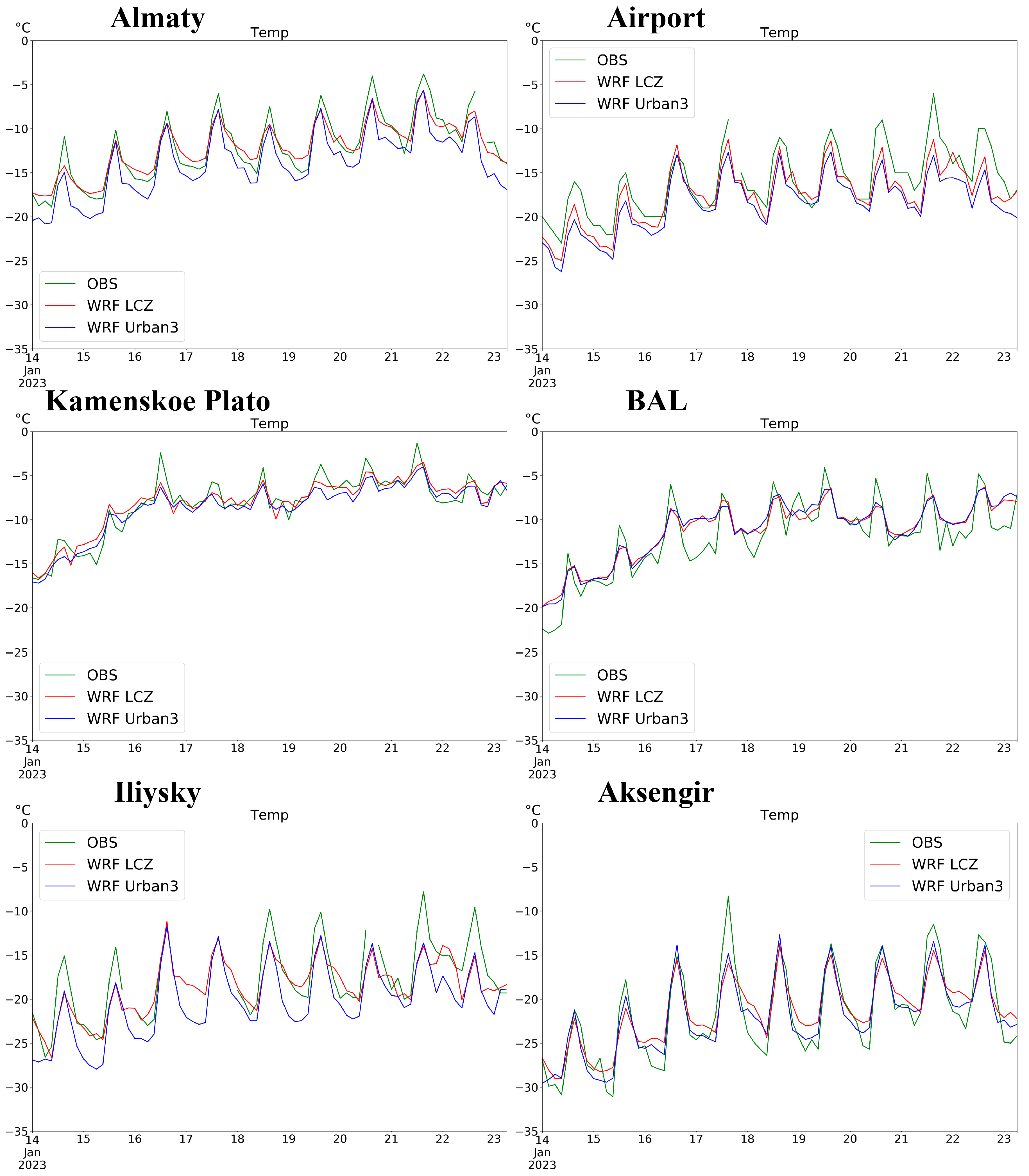
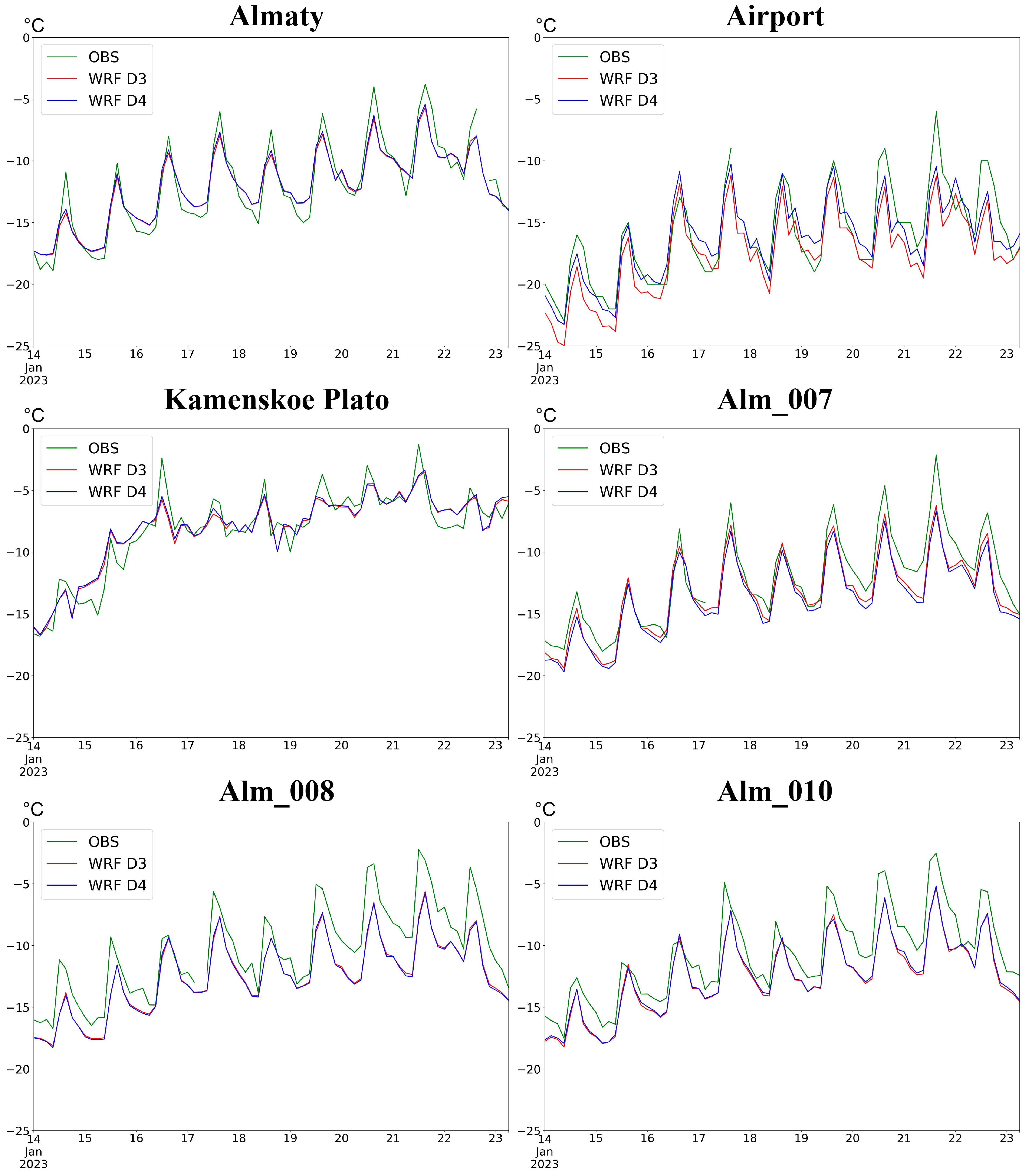
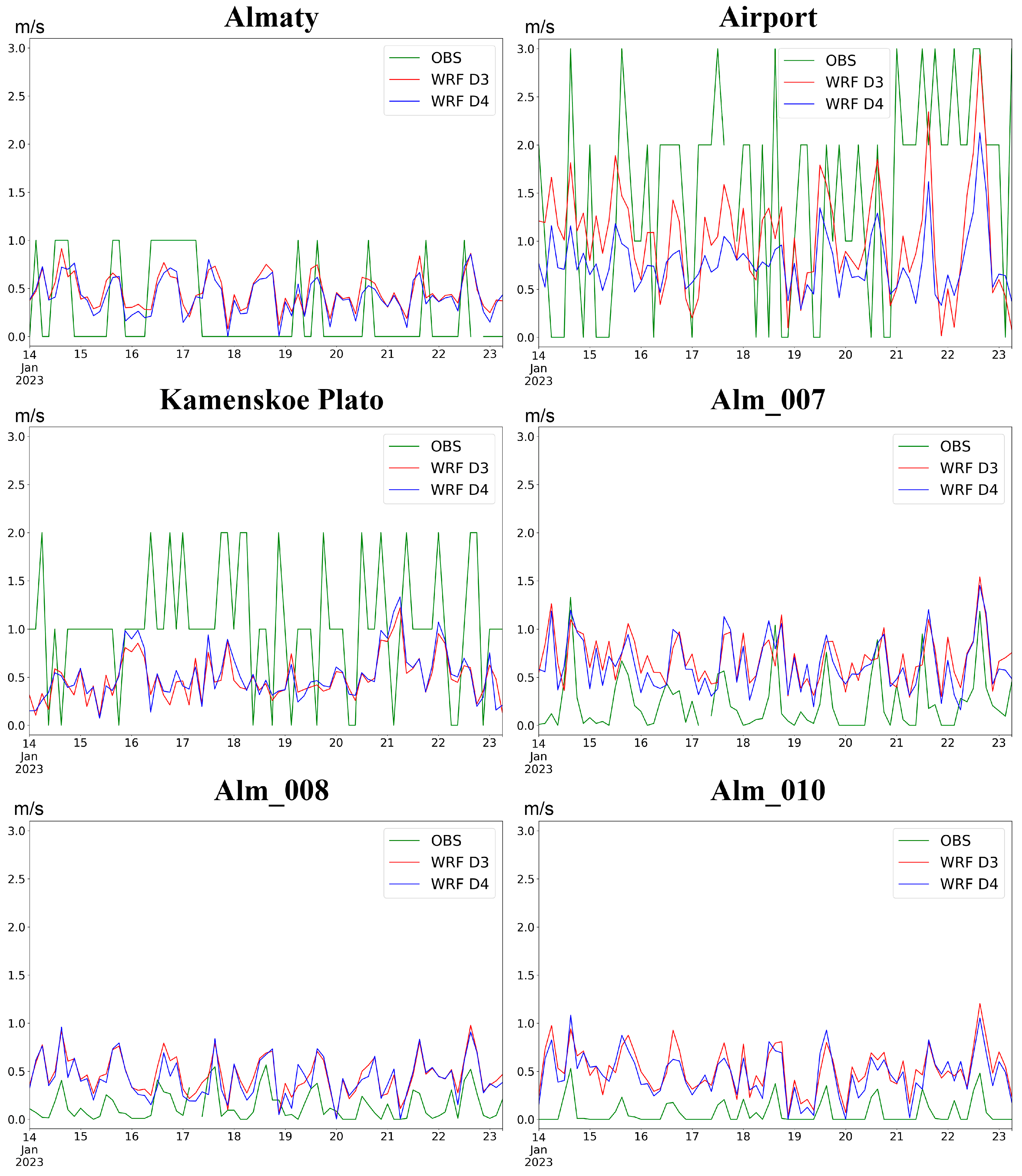
3.3. Comparison of High-Resolution Data with Meteorological Observation Data

The verification of the obtained results was performed by comparing the data of D3 and D4 domains with field measurements of temperature and wind speed. The analysis of wind direction was not performed due to very low speeds.

Table 4. Evaluation of experiment accuracy for D3 and D4 domains.

Name	Coordinates		BIAS_T, °C		MAE_T, °C		RMSE_T, °C		BIAS_v, m/s		MAE_v, m/s		RMSE_v, m/s
	Lat	Lon	D3	D4	D3	D4	D3	D4	D3	D4	D3	D4	D3	D4
Almaty	43.24	76.93	−0.10	−0.03	0.92	0.92	1.15	1.12	0.11	0.07	0.30	0.26	0.55	0.51
Airport	43.36	77.00	−1.56	−0.41	1.81	1.31	2.28	1.70	−0.47	−0.61	0.96	1.01	1.21	1.26
Kamenskoe Plato	43.18	76.97	0.03	0.12	0.93	0.94	1.18	1.18	−0.63	−0.56	0.76	0.75	1.01	0.98
Alm-007	43.28	76.87	−1.03	−1.42	1.15	1.48	1.44	1.75	0.50	0.43	0.60	0.53	0.70	0.65
Alm-008	43.25	76.88	−1.99	−2.04	2.00	2.05	2.37	2.41	0.24	0.20	0.34	0.33	0.50	0.49
Alm-010	43.24	76.83	−1.77	−1.69	1.80	1.73	2.06	2.00	0.41	0.40	0.44	0.42	0.63	0.61
Mean			1.08	0.95	1.44	1.40	1.75	1.70	0.39	0.38	0.57	0.55	0.77	0.75

illustrates the mean absolute error (BIAS), mean absolute error (MAE), and mean square error for three meteorological stations and three automated monitoring stations. The table shows that, on average, the correlation coefficients for temperature and wind speeds for the D4 domain are lower than for the D3 domain. Minor differences exist between the data for D3 and D4 domains regarding observation points.

Figure 9 compares simulated and observed temperatures at various meteorological stations. The model accurately captures the daily temperature cycle (diurnal variation) at both Almaty and Kamenskoe Plato stations for both model domains. However, it underestimates the magnitude of temperature fluctuations (amplitude) by 1–2 °C. The simulated temperature at the Airport station is approximately 2 °C colder than the observed data. This discrepancy is likely due to errors in assigning local climate zones during the cell generalization. In contrast, temperatures measured at the Alm-008, Alm-010, and Alm-007 monitoring stations are higher than the simulated values. These stations likely record slightly higher temperatures (2–3 °C for Alm-008 and Alm-010, and 1–1.5 °C for Alm-007) because their sensors are near heat-emitting structures, influencing the ambient air temperature measurements.

The analysis of wind speed plots in Figure 10 reveals that the model performs well in capturing wind speed fluctuations at both observation points for the D3 and D4 domains, except for the Airport station, where the correlation for the D4 domain shows some deterioration. Notably, the Almaty meteorological station in the D4 domain aligns best with observed data. Wind speeds are slightly lower (0.5 m/s) compared to the D3 domain for the Airport station. This minor difference might stem from biases introduced during LCZ class when generalizing cells. The model consistently underestimates wind speeds at Kamenskoe Plato for both domains. This is likely due to the complex topography surrounding the weather station, which the model might not fully capture. It is noteworthy that the sensor limitations are at the Alm-007, Alm-008, and Alm-010 monitoring stations. These stations share a sensor unit located only 2.5 m above ground level. Consequently, their measured wind speeds are very low (no more than 0.5 m/s). In contrast, the WRF model calculates wind velocities at a height of 10 m, resulting in a wider range of values that can reach over 1 m/s.

As discussed earlier, discrepancies between simulations and observations might arise from inaccuracies in determining local climate zones during cell generalization.

Table 5. Characteristics of meteorological observation station locations in terms of LCZ.

Name	Lat	Lon	LCZ	LCZ_D3	LCZ_D4
Almaty	43.24	76.93	LCZ 5	LCZ 5	LCZ 5
Airport	43.36	77.00	LCZ 6	LCZ 10	LCZ C
Kamenskoe Plato	43.18	76.97	LCZ 9	LCZ A	LCZ 9
Alm-007	43.28	76.87	LCZ 10	LCZ A	LCZ 7
Alm-008	43.25	76.88	LCZ 5	LCZ 5	LCZ 5
Alm-010	43.24	76.83	LCZ 5	LCZ 5	LCZ 5

presents the characteristics of meteorological station locations, considering the LCZ classification from the original 90 m resolution map (LCZ). The table also shows how these characteristics change when cell sizes are generalized to 1 km in the D3 domain (LCZ_D3) and 333 m in the D4 domain (LCZ_D4).

Data from weather stations are missing from Figure 9 and Figure 10 due to reasons beyond our control. This may be related to a failure during the observation process or problems with transmitting meteorological data to the server.

Table 5 reveals that automatic cell generalization can alter the original LCZ classification assigned to meteorological stations. This is particularly evident for the Airport and Alm-007 stations, where LCZ classes differ across all three resolutions. Similarly, the Kamenskoe Plato station shows a discrepancy between the D3 and D4 domains. This is shown in more detail in Figure 11. This mismatch in LCZ classes likely contributes to the divergence observed in comparative plots, where simulations from different domains exhibit greater differences. Conversely, when LCZ classes remain consistent across domains (as in some cases), the simulation results from the D3 and D4 domains are nearly identical (Figure 9 and Figure 10).

Table 5 shows some inconsistencies in LCZ data at specific points (Airport, Alm-007, Kamenskoe Plato). However, comparing the simulation results and data in Figure 9 and Figure 10 shows that the model can capture wind and temperature patterns in Almaty. This is true for both the D3 and D4 domains. This suggests that neighboring cells with consistent LCZ classifications might influence the overall results, mitigating the errors introduced by land use map generalization and smoothing out temperature and wind inaccuracies at specific stations. This suggests that nearby cells with consistent LCZ classifications might influence the overall results. They could also reduce the errors from land use map simplification. In addition, they could smooth out temperature and wind inaccuracies at specific stations.

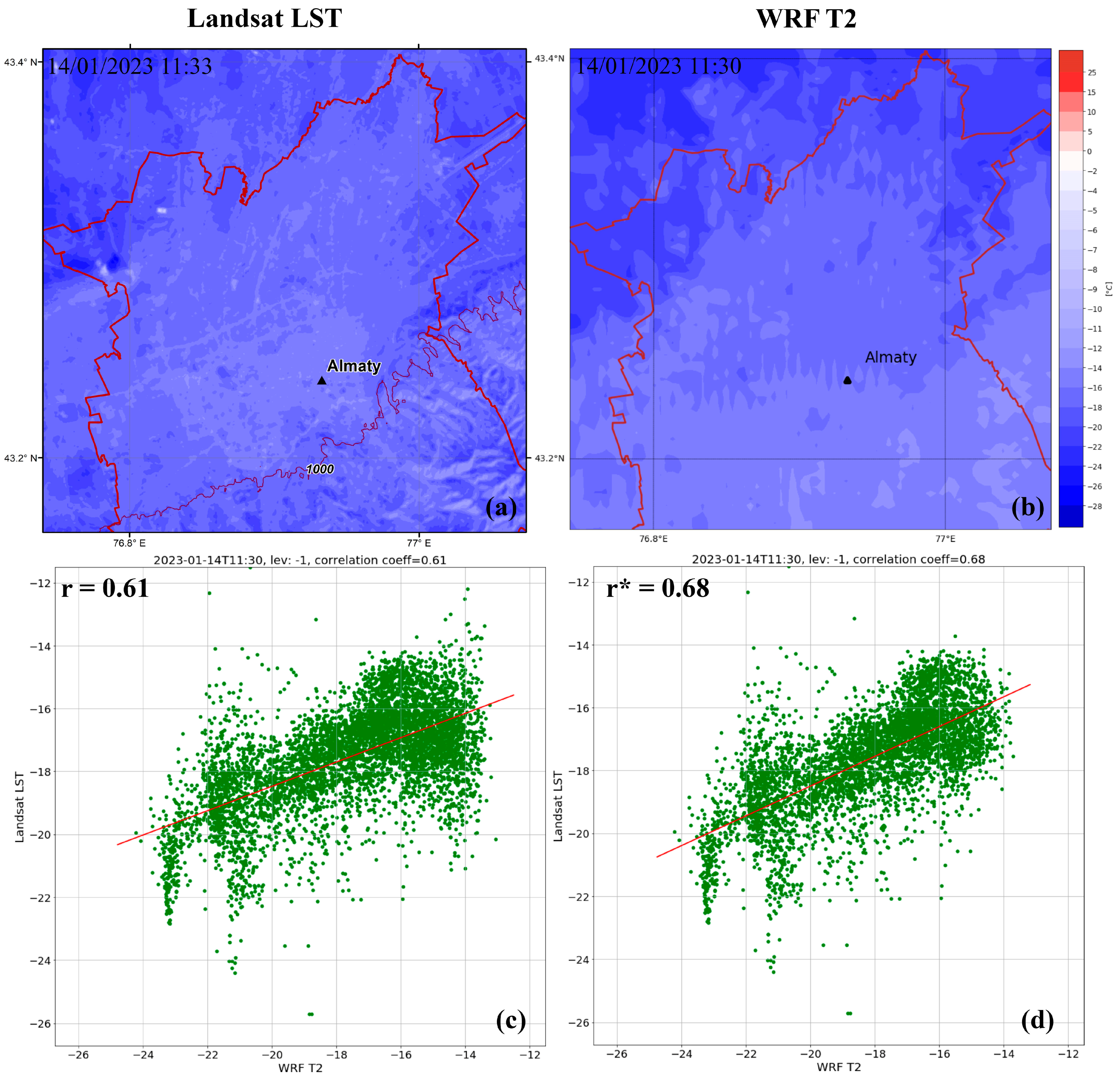
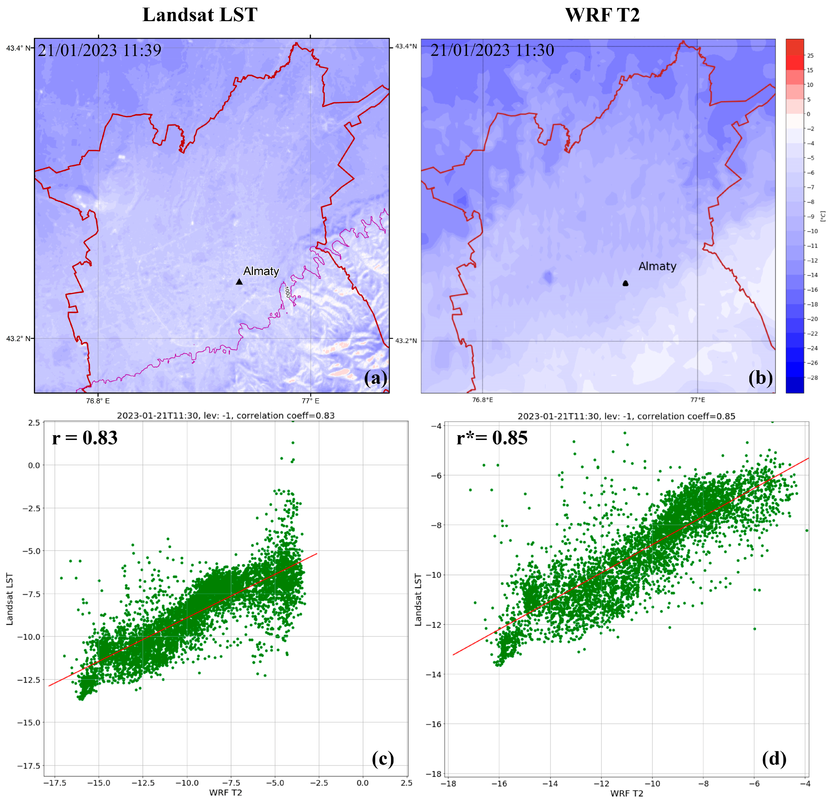
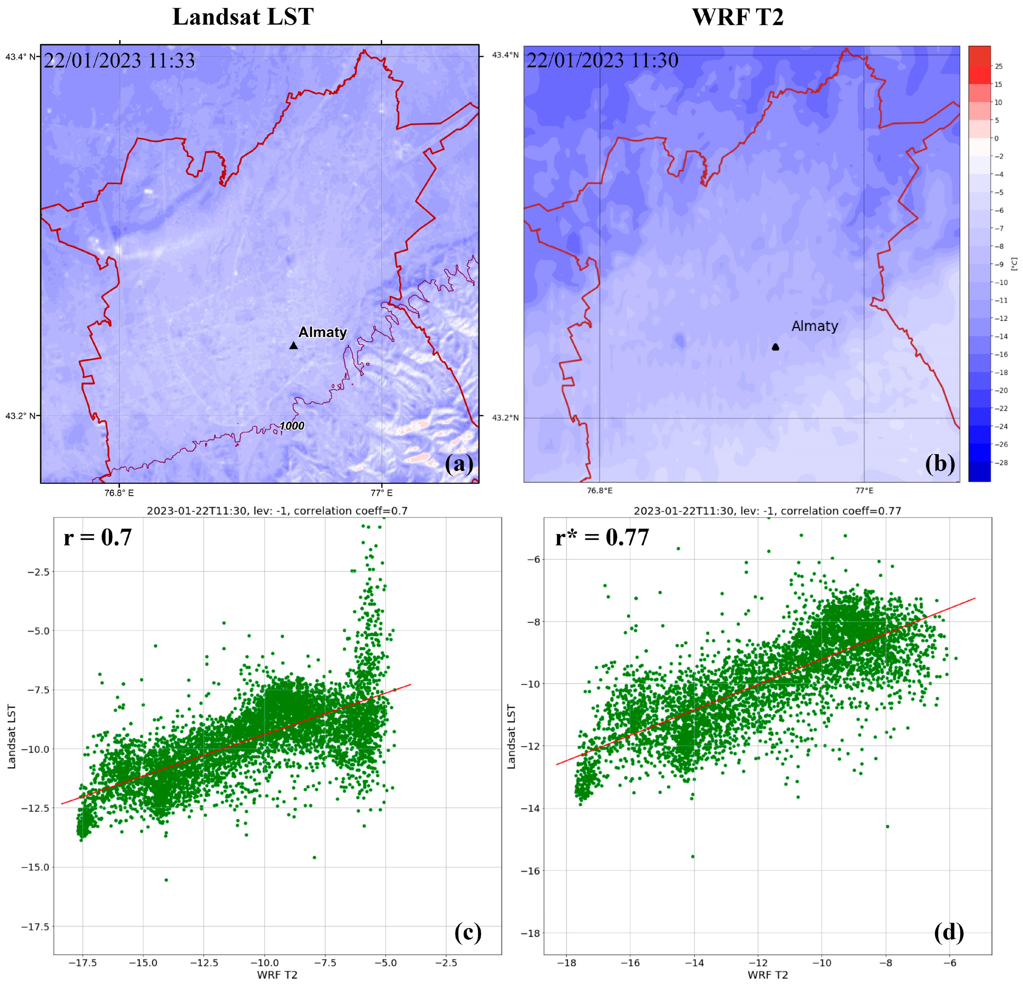
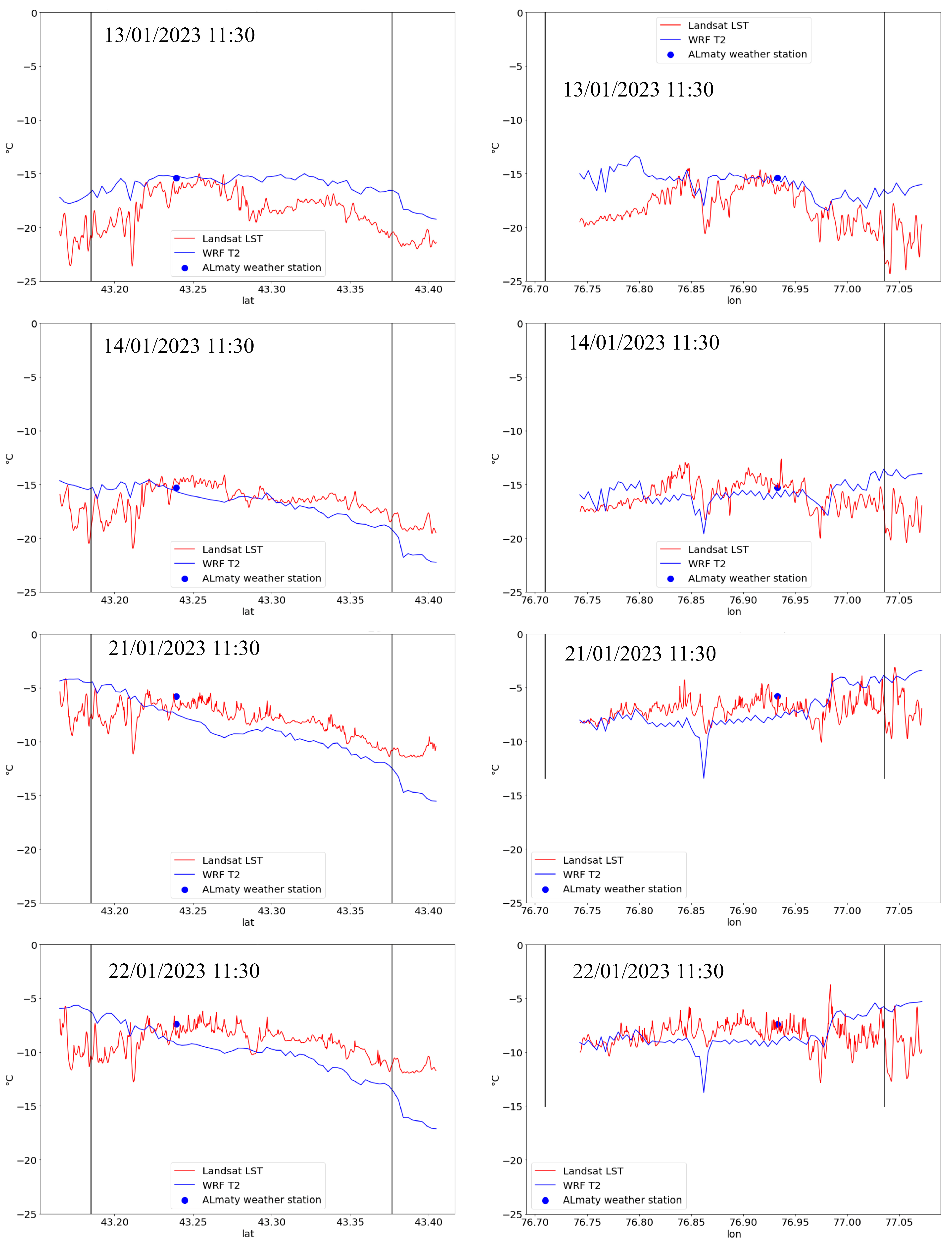
3.4. Comparison of Temperature Regime with Remote Sensing Data

Figure 12, Figure 13, Figure 14 and Figure 15 present the correlation relationships between land surface temperature (LST) derived from satellite remote sensing data and near-surface air temperature simulated by WRF. The calculated correlation coefficients (r) between observational data and simulation results range from 0.61 to 0.83. The largest scatter of values is observed for mountainous areas. This is explained by the fact that the satellite images were taken on clear sunny days with anticyclonic conditions close to noon (11:30 local time), when the heating of mountain slopes strongly depends on solar exposure, and the temperature difference between illuminated and shaded areas reaches maximum values. If we consider only the flat territory (i.e., limiting ourselves to the territory with elevations up to 1000 m above sea level), then the correlation coefficient r* increases to values from 0.68 to 0.85 (see Figure 12, Figure 13, Figure 14 and Figure 15). It should be noted that an increase in the temperature of the street road network is traced on satellite images with the temperature of the Earth’s surface, while the WRF model, when calculating air temperature, considers the heating of urban infrastructure objects indirectly through the characteristics of urban LCZ classes, which is not so clearly reflected in the temperature field.

To better compare remote sensing data and modeling results, temperature profiles were constructed along south–north (left-hand graphs) and west–east (right-hand graphs) cross-sections through the Almaty meteorological station point (Figure 16).

The vertical black lines on these graphs represent the boundaries of the urbanized part of the city. The figures reveal that the simulation results correspond to the remote sensing data and reflect the main features of the thermal fields in winter under anticyclonic conditions. The best correspondence is observed in the south–north direction, where the curves smoothly intersect the city with a gradual cooling of the air in its northern part. It is noteworthy that in the simulations, the frozen Lake Sayran, located in the city center, is highlighted on the west–east profiles as a point of sharp cooling. Satellite imagery also records this lake but with a much smaller temperature drop.

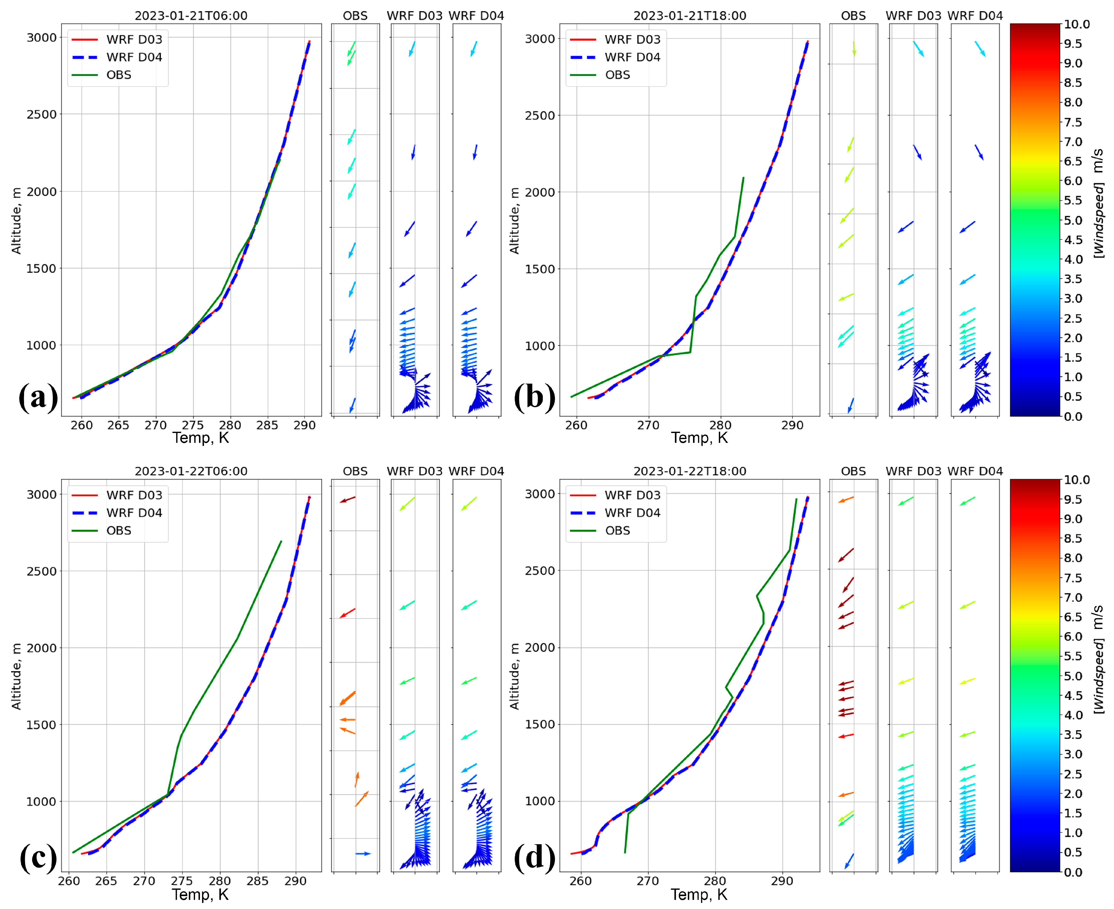
3.5. Comparison with Radiosounde Data

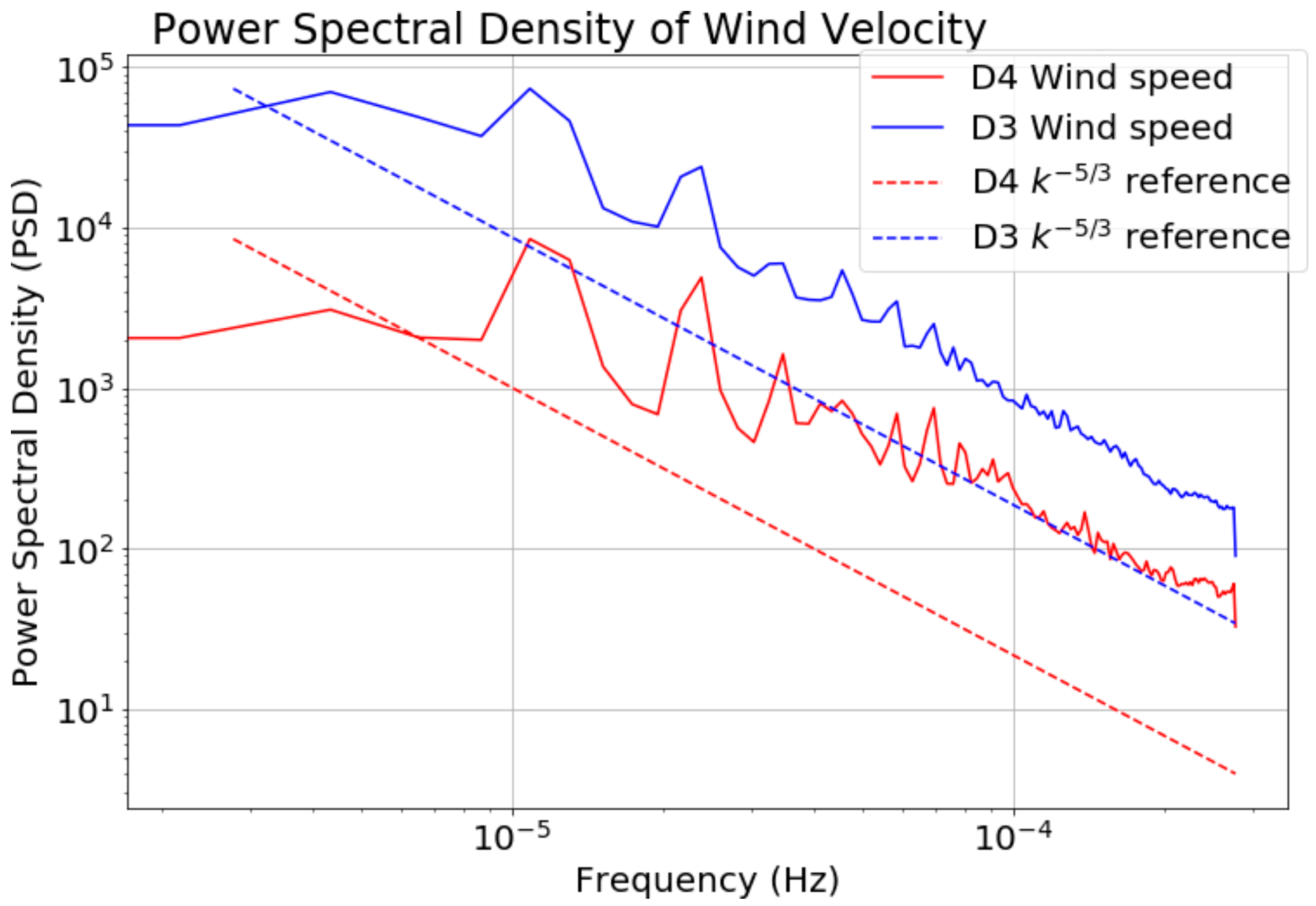
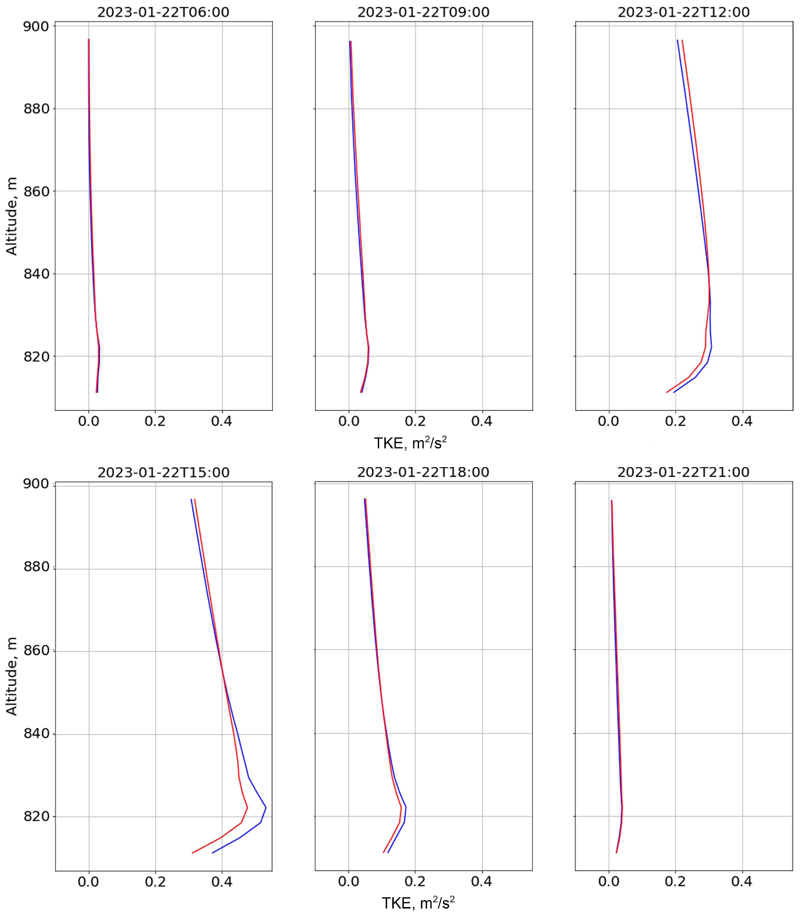
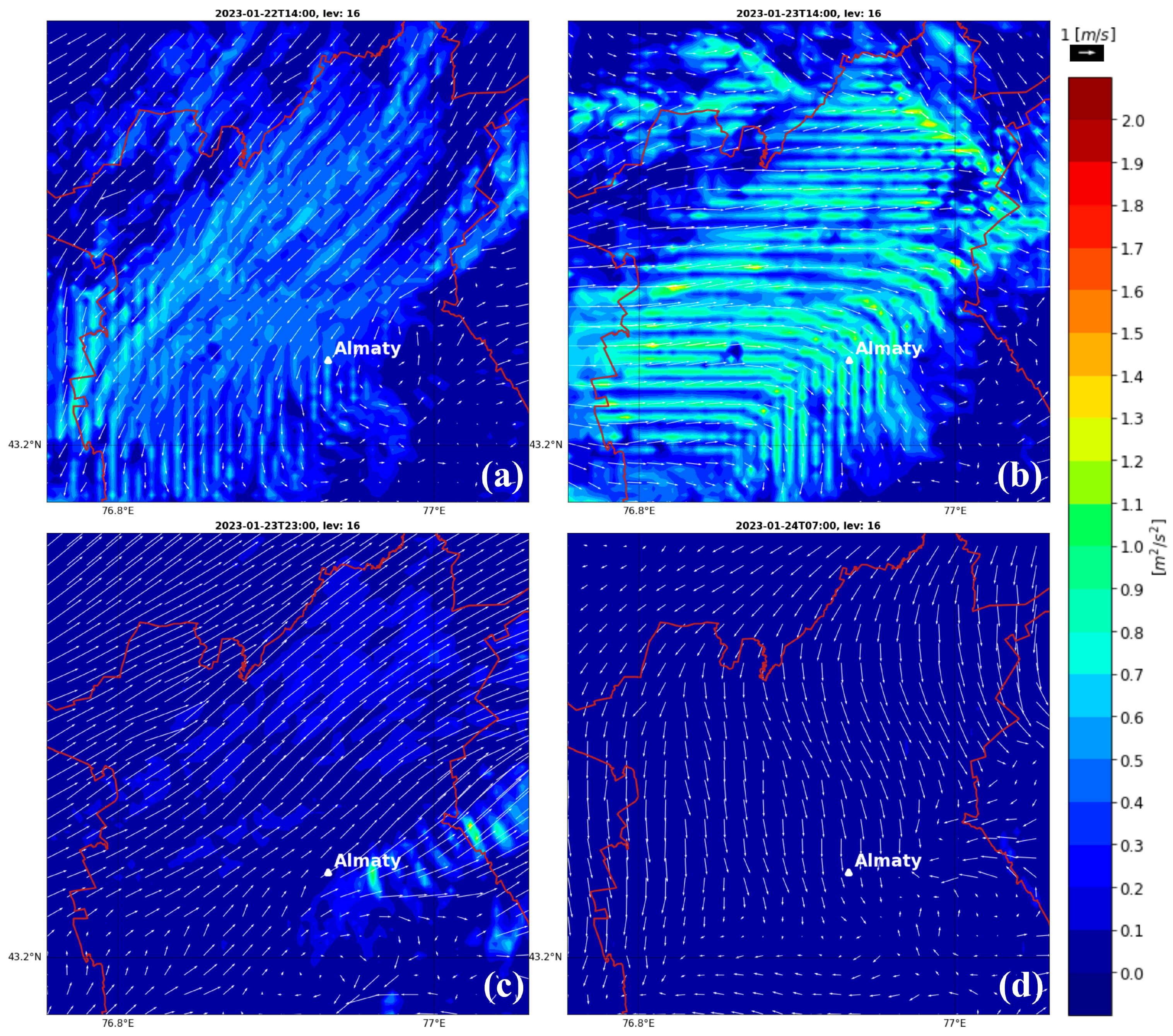
Researchers use various methods to obtain data on the vertical structure of wind flows [6,9,57]. Unfortunately, in the vicinity of Almaty, there is only one aerological station that launches radiosondes twice a day—at 6:00 and 18:00 local time [54]. Figure 17 compares aerological observations of potential temperature and wind speed for the D3 and D4 domains alongside the corresponding data simulated by the model. The figure shows that (1) the downscaling procedure did not introduce any changes in the calculations of the boundary layer; (2) the results of modeling the nocturnal stably stratified boundary layer are in good agreement with the radiosonde measurements; (3) the WRF model does not reflect the multilayer structure of the inversion in the upper layers of the boundary layer, as recorded by radiosonde data.

3.6. Turbulence

A key characteristic of turbulence in the atmosphere is the power spectral density (PSD) of wind velocity at a height of 10 m, where human life is concentrated. Figure 18 shows such spectra constructed using the Welch method [55] based on the results of calculating wind speed on a horizontal grid with a step of 1 km (blue line) and on a denser grid with a step of 333 m (red line) averaged over the area of the D4 domain.

Analysis of the energy spectrum reveals that the model in this study accurately represents the damping of low-frequency (10⁻⁵ to 10⁻⁴ Hz) turbulence energy generated by solar heating near the surface, as well as the subsequent dissipation of pulsating energy consistent with the Kolmogorov spectrum k^−5/3.

The turbulent energy spectra derived from the calculation results across various grids exhibit consistent pulsation energy-damping characteristics. However, the magnitude of this energy on the dense grid (333 m) is less than on the sparse grid (1 km) across the entire spectral range. This difference is due to the averaging of small-scale turbulent processes and energy accumulation on a 1 km grid. In contrast, on the dense grid, lower energy is accumulated due to small-scale processes, which leads to a more efficient turbulent cascade that distributes energy across the entire spectrum.

Meteorological processes in the atmosphere of Almaty city during the anticyclonic period have a daily periodicity [31,58,59]. Nocturnal (21:00–09:00) and daytime (09:00–21:00) phases of atmospheric processes are observed, and the daytime phase can be divided into morning (09:00–12:00) and evening (16:00–21:00) periods when, following the solar cycle, processes in the subinversion layer grow and fade. These phases and periods are effectively traced when analyzing the results of modeling turbulent processes.

Figure 19 presents vertical profiles of turbulent kinetic energy (TKE) at different times of day (averaged over the area of the D4 domain). As can be seen from the figure, the nocturnal stagnant state of a stably stratified atmosphere is characterized by the absence of turbulence, TKE is near zero practically over the entire height of the surface layer (Figure 19, 6:00). In the morning, with the rising of the sun, the underlying surface and the adjacent air layer (urban canopy layer) are heated, which leads to turbulent mixing in this layer (Figure 19, 9:00). Further, this process develops, the mixing layer increases and reaches a maximum (about 900 m above sea level) by the end of the morning period (Figure 17, 12:00 and 15:00). As solar activity decreases in the evening, the mixing layer decreases and completely disappears by sunset (Figure 19, 18:00 and 21:00). It should be noted that the calculation results of the vertical TKE profiles for D3 and D4 domains are in good agreement with each other. The largest difference of 0.05 m²/s² occurs at the moment of maximum TKE activity, and the pulsating energy is higher when calculated on a grid with a step of 1 km (D3 domain) than on a denser grid with a step of 333 m (D4 domain).

The calculation results presented above define the integral characteristics of the mixing layer. Vertical wind speed profiles reveal a more nuanced view of turbulence within this layer. Such a section is presented in Figure 20. It refers to a typical day of a January anticyclone when turbulence reaches its maximum value. As can be seen from the figure, two wind processes are implemented in the surface layer of the atmosphere: an anabatic flow of warm air into the mountains (lower level) and a chain of vertical vortices of low intensity, covering the entire mixing layer. Therefore, the turbulence model adopted in the work implements the mixing process in the form of cellular convection from solar heating. The frequency of the system of small vortices corresponds to the horizontal step of the computational grid. When these processes (vertical ascent and mountain flow) superimpose, a current may arise that combines the air mass transport by local winds with vertical mixing.

Vortex structures appear on horizontal sections of the TKE field (Figure 21) as vortex tracks following the streamlines of local winds. These calculations effectively illustrate the complex structure of local winds under anticyclonic conditions. The figure shows various variants of vortex tracks that arose under the influence of mountain–valley circulation and latitudinal transfer (Figure 19a,b). At night, a katabatic wind descends from mountains with almost no turbulence. (Figure 19c). In the morning, vortex streets are also absent, indicating the importance of atmospheric stability regardless of wind direction (Figure 19d).

Therefore, the results of the TKE calculations demonstrate that the high-resolution WRF model with the adopted configuration of parameterization methods adequately reflects the typical diurnal variations of meteorological processes in the atmosphere of Almaty during the anticyclonic period.

4. Discussion

Like any study involving modeling, this work has certain uncertainties and limitations.

Uncertainties are directly related to the modeling of atmospheric processes. With a wide range of parameterization methods for atmospheric processes such as the boundary layer, turbulence, convection, cloud microphysics, etc., the WRF model has its errors and simplifications compared to the real atmosphere. In our opinion, the main uncertainty in the high-resolution WRF model is turbulence since, with an increase in resolution to 333 m, the physics of modeling falls into a “gray zone” where neither planetary boundary layer modeling nor large eddy simulation (LES) is fully suitable. In this study, the PBL parameterization scheme was used, but in the future, experiments will be conducted using new boundary layer parameterization schemes described in [9], as well as LES, and varying the parameters related to turbulence.

Errors or inaccuracies in the initial and boundary data can lead to errors in the modeling. In our work, we use initial and boundary conditions from the NCEP GFS global meteorological database, which have a spatial resolution of 0.25° × 0.25° and a time step of 3 h. Increasing the resolution can, to some extent, reduce errors in the modeling results; therefore, it is planned to consider using input meteorological parameters with a higher spatial and temporal resolution, for example, data from the ICON model [60].

Complex terrain also leads to errors in modeling the atmosphere of Almaty. Uncertainties arise when generalizing the 30 m resolution digital elevation model to the WRF resolution (1 km, 333 m), as a result of which, within the high mountainous regions, there are areas with very sharp height differences, where numerical errors arise, especially when calculating wind velocity. The correction of the domain D3 boundaries carried out within the framework of this work along natural gorges reduced the number of such areas but did not eliminate them. In the future, this work is planned to continue.

The land use map with the classification of urban classes can also lead to errors in modeling. Significant uncertainties are introduced by the procedure for generalizing land use data from the original 90 m to the model resolution (1 km and 333 m). In the future, it is planned to improve the land use map, for example, by increasing its resolution and refining classes, as well as improving the process of generalizing the land use map for WRF. In addition, as a future step, it is planned to jointly use the urban canopy scheme and the building energy performance model (BEP + BEM). This will help to model building energy consumption and will be used in the future for microscale modeling.

The limitations of our study are related to the scarcity and inaccuracy of ground observations necessary for model validation. Increasing the network of meteorological observations (for example, increasing the number of automatic monitoring or weather stations) will help improve the operation of WRF. Certain steps in this direction have already been taken; automatic weather stations have been installed, and data are being collected for further research.

To mitigate the limitations associated with the resolution of the computational grid, we plan to increase the vertical resolution of the model while choosing the optimal number of vertical layers to slightly increase the computational resources and memory for storing and processing the obtained results. Increasing the number of vertical layers will allow further smoothing of the effects of the “gray zone” and obtain more accurate results, which will subsequently become input data for microscale modeling at the level of quarters and buildings.

5. Conclusions

This study presents the results of high-resolution (333 m) WRF modeling of the atmosphere for the city of Almaty using LCZ as land use data. A detailed local climate zone map for Almaty was constructed leveraging the LCZ Generator tool. It includes 10 types of urban development and seven types of natural landscapes, providing the WRF model with sufficiently detailed information about the underlying surface.

For WRF modeling, the period from 13 to 23 January 2023 was chosen, characterized by environmentally unfavorable meteorological conditions of the Asian anticyclone, typical for the winter in the studied territory.

Comparative analysis of the results of WRF modeling with meteorological observation data (six Kazhydromet meteorological stations) showed that modeling using LCZs provides a better match in temperature for five meteorological stations and in wind speed for four, excluding high-mountain ones. This is illustrated by the mean (BIAS), absolute (MAE), and root mean square (RMSE) errors, as well as graphs of temperature, wind speed, and wind roses.

Limited meteorological data prompted additional analysis of wind regime simulations using Landsat remote sensing data. For this purpose, the output meteorological parameters of WRF were employed in the SILAM model, and the results obtained were compared with the plumes of pollutant transport, clearly recorded on satellite images in the visible range. The analysis showed a direction of plume propagation similar to that of the remote sensing data. This indicates that the wind calculated in WRF corresponds to the real wind regime. Furthermore, both the images and the calculations demonstrate the dominant latitudinal transport, which occurs in the northern part of the city with a characteristic change in wind direction from east to west and vice versa.

Comparative analysis of modeling results for the D3 domain with a 1 km resolution and the D4 domain with a 333 m resolution with meteorological observation data demonstrates the ability of the WRF model to adequately represent the wind and thermal regimes of the city of Almaty at high resolution. Minor discrepancies between the modeling results of D3 and D4 domains and field measurements can be attributed to both generalization inaccuracies in LCZ determination and the field measurements. In particular, the analysis revealed a significant influence of station location on monitoring results from automatic stations. Stations near buildings experienced a pronounced dampening of local wind speeds and an overestimation of air temperatures.

Analysis of thermal fields revealed a strong correlation between land surface temperature (LST) derived from remote sensing data and 2 m air temperature (T2) simulated by WRF with a high resolution of 333 m. The correlation coefficient (r) ranged from 0.6 to 0.83. The highest dispersion of values was observed in mountainous areas, where the temperature difference between illuminated and shaded areas at the time of imaging reached maximum values.

Comparative analysis of aerological measurements of potential temperature and wind speed with similar calculated data for domains D3 and D4 revealed that the downscaling procedure did not introduce any changes in the boundary layer calculations. The modeling results for the nocturnal stably stratified boundary layer showed good agreement with radiosonde measurements. However, the WRF model failed to reproduce the multi-layered inversion structure in the upper boundary layer, as observed by radiosonde data.

Analysis of turbulence processes revealed that the adopted model effectively describes the attenuation of low-frequency turbulence energy and the subsequent dissipation of pulsating energy. The results of TKE calculations demonstrated that the model accurately captures the diurnal variations of meteorological processes in the atmosphere of Almaty City during the anticyclonic period.

Thus, the conducted research has shown that the WRF model adequately reflects the wind and thermal regimes of the city of Almaty, both in domain D3 with a resolution of 1 km and in domain D4 with a higher resolution of 333 m. This opens up prospects for the development of a hybrid system with a CFD (Computational Fluid Dynamics) class model capable of modeling atmospheric processes at the level of individual buildings or city blocks, using initial and boundary conditions formed in WRF in domain D4.

References

1. Skamarock, W.C.; Klemp, J.B.; Dudhia, J.B.; Gill, D.O.; Barker, D.M.; Duda, M.G.; Huang, X.-Y.; Wang, W.; Powers, J.G. A Description of the Advanced Research WRF Model Version 4.3 (No. NCAR/TN-556+STR). NCAR Tech. Note 2021. [Google Scholar] [CrossRef]
2. Zakarin, E.A.; Baklanov, A.A.; Balakay, L.A.; Dedova, T.V.; Bostanbekov, K.A. Simulation of Air Pollution in Almaty City under Adverse Weather Conditions. Russ. Meteorol. Hydrol. 2021, 46, 121–128. [Google Scholar] [CrossRef]
3. Zakarin, E.; Baklanov, A.; Balakay, L.; Dedova, T.; Bostanbekov, K. Modeling of the Calm Situations in the Atmosphere of Almaty. Asian J. Atmos. Environ. 2022, 16, 14–31. [Google Scholar] [CrossRef]
4. Berardi, U.; Jandaghian, Z.; Graham, J. Effects of Greenery Enhancements for the Resilience to Heat Waves: A Comparison of Analysis Performed through Mesoscale (WRF) and Microscale (Envi-Met) Modeling. Sci. Total Environ. 2020, 747, 141300. [Google Scholar] [CrossRef]
5. Wong, N.H.; He, Y.; Nguyen, N.S.; Raghavan, S.V.; Martin, M.; Hii, D.J.C.; Yu, Z.; Deng, J. An Integrated Multiscale Urban Microclimate Model for the Urban Thermal Environment. Urban Clim. 2021, 35, 100730. [Google Scholar] [CrossRef]
6. Bauer, H.S.; Muppa, S.K.; Wulfmeyer, V.; Behrendt, A.; Warrach-Sagi, K.; Späth, F. Multi-Nested WRF Simulations for Studying Planetary Boundary Layer Processes on the Turbulence-Permitting Scale in a Realistic Mesoscale Environment. Tellus Ser. A Dyn. Meteorol. Oceanogr. 2020, 72, 1–28. [Google Scholar] [CrossRef]
7. Zhu, D.; Zhou, X.; Cheng, W. Water Effects on Urban Heat Islands in Summer Using WRF-UCM with Gridded Urban Canopy Parameters—A Case Study of Wuhan. Build. Environ. 2022, 225, 109528. [Google Scholar] [CrossRef]
8. Moya-Álvarez, A.S.; Martínez-Castro, D.; Kumar, S.; Estevan, R.; Silva, Y. Response of the WRF Model to Different Resolutions in the Rainfall Forecast over the Complex Peruvian Orography. Theor. Appl. Clim. 2019, 137, 2993–3007. [Google Scholar] [CrossRef]
9. Hope, A.P.; Lopez-Coto, I.; Hajny, K.; Tomlin, J.M.; Kaeser, R.; Stirm, B.; Karion, A.; Shepson, P.B. Analyzing “Gray Zone” Turbulent Kinetic Energy Predictions in the Boundary Layer from Three WRF PBL Schemes over New York City and Comparison with Aircraft Measurements. J. Appl. Meteorol. Clim. 2024, 63, 125–142. [Google Scholar] [CrossRef]
10. Bougeault, P.; Lacarrere, P. Parameterization of Orography-Induced Turbulence in a Mesobeta-Scale Model. Mon. Weather Rev. 1989, 117, 1039–1057. [Google Scholar] [CrossRef]
11. Martilli, A.; Clappier, A.; Rotach, M.W. An Urban Surface Exchange Parameterisation for Mesoscale Models. Bound. Layer Meteorol. 2002, 104, 261–304. [Google Scholar] [CrossRef]
12. Martilli, A.; Clarke, S.G.; Tewari, M.; Manning, K.W. Description of the Modification s Made in WRF.3.1 and Short User’s Manual of BEP; National Center for Atmospheric Research: Boulder, CO, USA, 2009. [Google Scholar]
13. Siewert, J.; Kroszczynski, K. Evaluation of High-Resolution Land Cover Geographical Data for the WRF Model Simulations. Remote Sens. 2023, 15, 2389. [Google Scholar] [CrossRef]
14. Golzio, A.; Ferrarese, S.; Cassardo, C.; Diolaiuti, G.A.; Pelfini, M. Land-Use Improvements in the Weather Research and Forecasting Model over Complex Mountainous Terrain and Comparison of Different Grid Sizes. Bound. Layer Meteorol. 2021, 180, 319–351. [Google Scholar] [CrossRef]
15. Stewart, I.D.; Oke, T.R. Local Climate Zones for Urban Temperature Studies. Bull. Am. Meteorol. Soc. 2012, 93, 1879–1900. [Google Scholar] [CrossRef]
16. WUDAPT. World Urban Database and Access Portal Tools. Available online: http://www.wudapt.org/ (accessed on 15 June 2024).
17. Lehnert, M.; Savić, S.; Milošević, D.; Dunjić, J.; Geletič, J. Mapping Local Climate Zones and Their Applications in European Urban Environments: A Systematic Literature Review and Future Development Trends. ISPRS Int. J. Geoinf. 2021, 10, 260. [Google Scholar] [CrossRef]
18. Vuckovic, M.; Hammerberg, K.; Mahdavi, A. Urban Weather Modeling Applications: A Vienna Case Study. Build. Simul. 2020, 13, 99–111. [Google Scholar] [CrossRef]
19. Brousse, O.; Martilli, A.; Foley, M.; Mills, G.; Bechtel, B. WUDAPT, an Efficient Land Use Producing Data Tool for Mesoscale Models? Integration of Urban LCZ in WRF over Madrid. Urban Clim. 2016, 17, 116–134. [Google Scholar] [CrossRef]
20. Zonato, A.; Martilli, A.; Di Sabatino, S.; Zardi, D.; Giovannini, L. Evaluating the Performance of a Novel WUDAPT Averaging Technique to Define Urban Morphology with Mesoscale Models. Urban Clim. 2020, 31, 100584. [Google Scholar] [CrossRef]
21. Molnár, G.; Gyöngyösi, A.Z.; Gál, T. Integration of an LCZ-Based Classification into WRF to Assess the Intra-Urban Temperature Pattern under a Heatwave Period in Szeged, Hungary. Theor. Appl. Clim. 2019, 138, 1139–1158. [Google Scholar] [CrossRef]
22. Mu, Q.; Miao, S.; Wang, Y.; Li, Y.; He, X.; Yan, C. Evaluation of Employing Local Climate Zone Classification for Mesoscale Modelling over Beijing Metropolitan Area. Meteorol. Atmos. Phys. 2020, 132, 315–326. [Google Scholar] [CrossRef]
23. McRae, I.; Freedman, F.; Rivera, A.; Li, X.; Dou, J.; Cruz, I.; Ren, C.; Dronova, I.; Fraker, H.; Bornstein, R. Integration of the WUDAPT, WRF, and ENVI-Met Models to Simulate Extreme Daytime Temperature Mitigation Strategies in San Jose, California. Build. Environ. 2020, 184, 107180. [Google Scholar] [CrossRef]
24. Richard, Y.; Emery, J.; Dudek, J.; Pergaud, J.; Chateau-Smith, C.; Zito, S.; Rega, M.; Vairet, T.; Castel, T.; Thévenin, T.; et al. How Relevant Are Local Climate Zones and Urban Climate Zones for Urban Climate Research? Dijon (France) as a Case Study. Urban Clim. 2018, 26, 258–274. [Google Scholar] [CrossRef]
25. Du, R.; Liu, C.H.; Li, X.X.; Lin, C.Y. Effect of Local Climate Zone (LCZ) and Building Category (BC) Classification on the Simulation of Urban Climate and Air-Conditioning Load in Hong Kong. Energy 2023, 271, 127004. [Google Scholar] [CrossRef]
26. Patel, P.; Karmakar, S.; Ghosh, S.; Niyogi, D. Improved Simulation of Very Heavy Rainfall Events by Incorporating WUDAPT Urban Land Use/Land Cover in WRF. Urban Clim. 2020, 32, 100616. [Google Scholar] [CrossRef]
27. System for Integrated ModelLling of Atmospheric CoMposition. Available online: https://silam.fmi.fi/ (accessed on 15 June 2024).
28. USGS EROS Archive-Landsat Archives-Landsat 8-9 Operational Land Imager and Thermal Infrared Sensor Collection 2 Level-1 Data. Available online: https://www.usgs.gov/centers/eros/science/usgs-eros-archive-landsat-archives-landsat-8-9-operational-land-imager-and (accessed on 10 April 2024).
29. Statistics of the Regions of the Republic of Kazakhstan. Almaty City. Available online: https://stat.gov.kz/en/region/almaty/ (accessed on 15 June 2024).
30. Vilesov, E.N. Climatic Conditions of Almaty; Al-Farabi Kazakh National University Press: Almaty, Kazakhstan, 2010. [Google Scholar]
31. Akhmetzhanov, H.A.; Shver, I.A. (Eds.) The Climate of Alma-Ata; Hydrometizdat: Leningrad, Russia, 1985. [Google Scholar]
32. Demuzere, M.; Kittner, J.; Bechtel, B. LCZ Generator: A Web Application to Create Local Climate Zone Maps. Front. Environ. Sci. 2021, 9, 637455. [Google Scholar] [CrossRef]
33. Fast and Easy Local Climate Zone Mapping. Available online: https://lcz-generator.rub.de/ (accessed on 15 June 2024).
34. Global Data Explorer (GDEx). Available online: https://lpdaac.usgs.gov/news/global-data-explorer-gdex-has-been-retired/ (accessed on 10 April 2024).
35. Global Forecast System (GFS). Available online: https://www.ncei.noaa.gov/products/weather-climate-models/global-forecast (accessed on 10 April 2024).
36. Jiménez, P.A.; Dudhia, J. On the Ability of the WRF Model to Reproduce the Surface Wind Direction over Complex Terrain. J. Appl. Meteorol. Climatol. 2013, 52, 1610–1617. [Google Scholar] [CrossRef]
37. Michelson, S.A.; Bao, J.W. Sensitivity of Low-Level Winds Simulated by the WRF Model in California’s Central Valley to Uncertainties in the Large-Scale Forcing and Soil Initialization. J. Appl. Meteorol. Clim. 2008, 47, 3131–3149. [Google Scholar] [CrossRef]
38. Bao, J.-W.; Michelson, S.A.; Persson, P.O.G.; Djalalova, I.V.; Wilczak, J.M. Observed and WRF-Simulated Low-Level Winds in a High-Ozone Episode during the Central California Ozone Study. J. Appl. Meteorol. Clim. 2008, 47, 2372–2394. [Google Scholar] [CrossRef]
39. Isaev, E.K.; Mostamandi, S.V.; Aniskina, O.G. Evaluation of the Influence of the Parameterization of Physical Processes in the WRF Hydrodynamic Model on the Quality of the Forecast of Atmospheric Processes in an Area with a Complex Topography Using the Example of the Territory of Kyrgyzstan. Uchenye Zap. RGGMU 2015, 30–41. [Google Scholar]
40. Lim, J.O.J.; Hong, S.Y.; Dudhia, J. The WRF-Single-Moment-Microphysics Scheme and Its Evaluation of the Simulation of Mesoscale Convective Systems. Bull. Am. Meteorol. Soc. 2004. [Google Scholar]
41. Kain, J.S.; Kain, J. The Kain-Fritsch Convective Parameterization: An Update. J. Appl. Meteorol. 2004, 43, 170–181. [Google Scholar] [CrossRef]
42. Iacono, M.J.; Delamere, J.S.; Mlawer, E.J.; Shephard, M.W.; Clough, S.A.; Collins, W.D. Radiative Forcing by Long-Lived Greenhouse Gases: Calculations with the AER Radiative Transfer Models. J. Geophys. Res. Atmos. 2008, 113, D13103. [Google Scholar] [CrossRef]
43. Monin, A.S.; Obukhov, A.M. Basic Laws of Turbulent Mixing in the Surface Layer of the Atmosphere. Contrib. Geophys. Inst. Acad. Sci. USSR 1954, 151, e187. [Google Scholar]
44. Ek, M.B.; Mitchell, K.E.; Lin, Y.; Rogers, E.; Grunmann, P.; Koren, V.; Gayno, G.; Tarpley, J.D. Implementation of Noah Land Surface Model Advances in the National Centers for Environmental Prediction Operational Mesoscale Eta Model. J. Geophys. Res. Atmos. 2003, 108. [Google Scholar] [CrossRef]
45. Weather for 241 Countries of the World. Available online: https://rp5.kz/Weather_in_the_world (accessed on 15 June 2024).
46. Wilks, D.S. Time Series. In International Geophysics; Academic Press: Cambridge, MA, USA, 2011; pp. 395–456. [Google Scholar]
47. Wang, D.; Liu, Y.; Yu, T.; Zhang, Y.; Liu, Q.; Chen, X.; Zhan, Y. A Method of Using WRF-Simulated Surface Temperature to Estimate Daily Evapotranspiration. J. Appl. Meteorol. Clim. 2020, 59, 901–914. [Google Scholar] [CrossRef]
48. Azargoshasbi, F.; Ashrafi, K.; Ehsani, A.H. Role of Urban Boundary Layer Dynamics and Ventilation Efficiency in a Severe Air Pollution Episode in Tehran, Iran. Meteorol. Atmos. Phys. 2023, 135, 35. [Google Scholar] [CrossRef]
49. Fu, P.; Weng, Q. Responses of Urban Heat Island in Atlanta to Different Land-Use Scenarios. Theor. Appl. Clim. 2018, 133, 123–135. [Google Scholar] [CrossRef]
50. Kaasik, M.; Prank, M.; Sofiev, M. Running the SILAM Model Comparatively with ECMWF and HIRLAM Meteorological Fields: A Case Study in Lapland. In Integrated Systems of Meso-Meteorological and Chemical Transport Models; Springer: Berlin/Heidelberg, Germany, 2011. [Google Scholar]
51. Prank, M.; Sofiev, M.; Kaasik, M.; Ruuskanen, T.; Kukkonen, J.; Kulmala, M. The Origins and Formation Mechanisms of Aerosol during a Measurement Campaign in Finnish Lapland, Evaluated Using the Regional Dispersion Model SILAM. In Air Pollution Modeling and Its Application XIX; NATO Science for Peace and Security Series C: Environmental Security; Springer: Cham, Switzerland, 2008. [Google Scholar]
52. Sofiev, M.; Siljamo, P.; Valkama, I.; Ilvonen, M.; Kukkonen, J. A Dispersion Modelling System SILAM and Its Evaluation against ETEX Data. Atmos. Environ. 2006, 40, 674–685. [Google Scholar] [CrossRef]
53. ECOSERVICE-S LLP. Available online: https://ecoservice.kz/ (accessed on 15 June 2024).
54. University of Wyoming Databases. Available online: http://weather.uwyo.edu/upperair/sounding.html (accessed on 10 April 2024).
55. Welch, P.D. The Use of Fast Fourier Transform for the Estimation of Power Spectra: A Method Based on Time Averaging Over Short, Modified Periodograms. IEEE Trans. Audio Electroacoust. 1967, 15, 70–73. [Google Scholar] [CrossRef]
56. Temirbekov, N.; Kasenov, S.; Berkinbayev, G.; Temirbekov, A.; Tamabay, D.; Temirbekova, M. Analysis of Data on Air Pollutants in the City by Machine-Intelligent Methods Considering Climatic and Geographical Features. Atmosphere 2023, 14, 892. [Google Scholar] [CrossRef]
57. Di Bernardino, A.; Mazzarella, V.; Pecci, M.; Casasanta, G.; Cacciani, M.; Ferretti, R. Interaction of the Sea Breeze with the Urban Area of Rome: WRF Mesoscale and WRF Large-Eddy Simulations Compared to Ground-Based Observations. Bound. Layer Meteorol. 2022, 185, 333–363. [Google Scholar] [CrossRef]
58. Helmholtz, N.F. Mountain-Valley Circulation of the Tien Shan Northern Slopes; Hydrometizdat: Leningrad, Russia, 1963. [Google Scholar]
59. Dedova, T.; Balakay, L.; Zakarin, E.; Bostanbekov, K.; Abdimanap, G. Investigating Stagnant Air Conditions in Almaty: A WRF Modeling Approach. Atmosphere 2024, 15, 633. [Google Scholar] [CrossRef]
60. Icon Model. Available online: https://www.icon-model.org/icon_model (accessed on 7 August 2024).
Figure 1. Example of identifiable Local Climate Zones for Almaty.
Atmosphere 15 00966 g001
Figure 2. Current map of Almaty suburbs in LCZ classification.
Atmosphere 15 00966 g002
Figure 3. Nested domain system and meteorological stations used for comparison with simulation results.
Atmosphere 15 00966 g003
Figure 4. Comparison of WRF modeling results using different underlying urban surface data with in situ air temperature measurements.
Atmosphere 15 00966 g004
Figure 5. Comparison of WRF modeling results using different underlying urban surface data with in situ wind speed measurements.
Atmosphere 15 00966 g005
Figure 6. Comparison of WRF modeling results using different underlying urban surface data with in situ wind direction measurements.
Atmosphere 15 00966 g006
Figure 7. Comparison of atmospheric pollution simulation results (b,d) with Landsat 8–9 data from 13 (a) to 14 (c) January 2023.
Atmosphere 15 00966 g007
Figure 8. Comparison of atmospheric pollution simulation results (b,d) with Landsat 8–9 data from 21 (a) to 22 (c) January 2023.
Atmosphere 15 00966 g008
Figure 9. Comparison of the results of the D3 and D4 domain calculations with meteorological observation data.
Atmosphere 15 00966 g009
Figure 10. Comparison of the results of the D3 and D4 domain calculations with meteorological observation data.
Atmosphere 15 00966 g010
Figure 11. Generalization in WRF of initial (a) LCZ maps for the D3 (b) and D4 (c) domains.
Atmosphere 15 00966 g011
Figure 12. Comparison of simulation results with remote sensing data from 13 January 2023: (a) Landsat-9 image in thermal band, (b) WRF-modeled air temperature, (c) correlation coefficient, (d) correlation coefficient on the flat territory, black triangle—Almaty weather station location.
Atmosphere 15 00966 g012
Figure 13. Comparison of simulation results with remote sensing data from 14 January 2023: (a) Landsat-9 image in thermal band, (b) WRF-modeled air temperature, (c) correlation coefficient, (d) correlation coefficient on the flat territory, black triangle—Almaty weather station location.
Atmosphere 15 00966 g013
Figure 14. Comparison of simulation results with remote sensing data from 21 January 2023: (a) Landsat-9 image in thermal band, (b) WRF-modeled air temperature, (c) correlation coefficient, (d) correlation coefficient on the flat territory, black triangle—Almaty weather station location.
Atmosphere 15 00966 g014
Figure 15. Comparison of simulation results with remote sensing data from 22 January 2023: (a) Landsat-9 image in thermal band, (b) WRF-modeled air temperature, (c) correlation coefficient, (d) correlation coefficient on the flat territory, black triangle—Almaty weather station location.
Atmosphere 15 00966 g015
Figure 16. Temperature profiles of Landsat LST and WRF T2.
Atmosphere 15 00966 g016
Figure 17. Comparison of potential temperature with radiosonde data: (a) 06:00, 21 January 2023; (b) 18:00, 21 January 2023; (c) 06:00, 22 January 2023; (d) 18:00, 22 January 2023.
Atmosphere 15 00966 g017
Figure 18. PSD of wind velocity at a height of 10 m for the D3 domain (blue line) and D4 domain (red line).
Atmosphere 15 00966 g018
Figure 19. Comparison of vertical TKE profiles for the D3 domain (blue line) and D4 domain (red line) on 22 January 2023.
Atmosphere 15 00966 g019
Figure 20. Vertical cross-section of wind field along the south–north line passing through Almaty weather station (lon 77.00, lat 43.36), 23 January 2023, 14:00.
Atmosphere 15 00966 g020
Figure 21. The horizontal sections of the TKE field on level 16 (~85 m), (a) 14:00, 22 January 2023; (b) 14:00, 23 January 2023; (c) 23:00, 23 January 2023; (d) 07:00, 24 January 2023.
Atmosphere 15 00966 g021