Weather Research and Forecasting Model (WRF) Sensitivity to Choice of Parameterization Options over Ethiopia

Abstract

Downscaling seasonal climate forecasts using regional climate models (RCMs) became an emerging area during the last decade owing to RCMs’ more comprehensive representation of the important physical processes at a finer resolution. However, it is crucial to test RCMs for the most appropriate model setup for a particular purpose over a given region through numerical experiments. Thus, this sensitivity study was aimed at identifying an optimum configuration in the Weather, Research, and Forecasting (WRF) model over Ethiopia. A total of 35 WRF simulations with different combinations of parameterization schemes for cumulus (CU), planetary boundary layer (PBL), cloud microphysics (MP), longwave (LW), and shortwave (SW) radiation were tested during the summer (June to August, JJA) season of 2002. The WRF simulations used a two-domain configuration with a 12 km nested domain covering Ethiopia. The initial and boundary forcing data for WRF were from the Climate Forecast System Reanalysis (CFSR). The simulations were compared with station and gridded observations to evaluate their ability to reproduce different aspects of JJA rainfall. An objective ranking method using an aggregate score of several statistics was used to select the best-performing model configuration. The JJA rainfall was found to be most sensitive to the choice of cumulus parameterization and least sensitive to cloud microphysics. All the simulations captured the spatial distribution of JJA rainfall with the pattern correlation coefficient (PCC) ranging from 0.89 to 0.94. However, all the simulations overestimated the JJA rainfall amount and the number of rainy days. Out of the 35 simulations, one that used the Grell CU, ACM2 PBL, LIN MP, RRTM LW, and Dudhia SW schemes performed the best in reproducing the amount and spatio-temporal distribution of JJA rainfall and was selected for downscaling the CFSv2 operational forecast.

1. Introduction

Advances in scientific understanding of the climate system and climate modeling have promoted seasonal forecasting to be a well-established operational area at several national centers around the world [1]. These centers (e.g., the National Center for Environmental Prediction, NCEP; the European Center for Medium Range Weather Forecast, ECMWF; Australian Bureau of Meteorology) are currently running seasonal forecasting systems (e.g., the Climate Forecast System version 2 (CFSV2 [2]), seasonal forecast system (SEAS5 [3]), and the Australian Ocean–Atmosphere Model for Climate Prediction (POAMA [4])) on a global scale. The seasonal forecast products of these systems provide reasonable global perspectives and outlooks of the climate several months in advance. However, despite their potential applications for different socioeconomic sectors, their usefulness has been limited in part due to their coarse spatial resolutions [1,5]. For the climate forecasts to be of practical societal value, the forecasts need to be issued at spatial scales appropriate to the decision maker or at the scale needed to use them as an input to impact models [5]. To address the scale problem and meet the needs for detailed regional information, downscaling seasonal forecasts by using regional climate models (RCMs) became an emerging area during the last decade [5,6,7].

Several studies around the world have demonstrated the potential advantages of using RCMs to downscale coarse-resolution climate predictions (e.g., [1,6,8,9,10,11,12,13,14]). Although fewer in number and scope (i.e., experimental and/or research only), RCMs have been tested over the Greater Horn of Africa (GHA) region. For example, in the study on dynamical seasonal hindcast over East Africa, Ref. [11] found that the Regional Climate Model system 4 (RegCM4) reproduced both the spatial and inter-annual variability of seasonal rainfall and captured the teleconnection between El Nino Southern Oscillation (ENSO) and regional rainfall structure. Ref. [15] evaluated downscaling of global seasonal hindcasts from the MPI-ESM global model using the COSMO-CLM (CCLM) RCM over East Africa during the summer season over a ten-year period (2000–2009). They found that while CCLM did not eliminate wet bias in summer precipitation over the Ethiopian highlands and certain lowland regions, it did provide added value in capturing extreme precipitation years, particularly in the Ethiopian highlands.

Despite the promising results and the widely accepted notion that RCMs can improve the simulation of precipitation compared with global forecasts owing to their more comprehensive representation of the important physical processes at a finer resolution [16,17,18], dynamical downscaling cannot be applied universally. This is due to a range of options available in RCMs for different physical and dynamical parameterizations. For example, the Weather Research and Forecasting (WRF) model (which is the focus of this study) currently provides more than 15 cumulus (CU), planetary boundary layer (PBL), and microphysics (MP) parameterization options [19]. These ranges of options are meant to allow users to select the physics and dynamics settings that optimize the model for their particular needs [20,21,22]. However, the variety of configurations in WRF can lead to varying results. The selection of an optimum combination of options depends on the quality of the lateral boundary condition, scales, geographic location, application, domain size, spin-up, vertical resolution, or nesting architecture [18], and any change in the configuration of these factors can lead to varying results. Hence, it is crucial to test for the most appropriate model set up for a particular purpose over a given region through numerical experiments [20]. Consequently, numerous sensitivity studies have been conducted over different parts of the world to identify the optimum WRF configuration (e.g., [21,23,24,25,26,27]).

Despite the crucial importance of sensitivity studies, only a handful of sensitivity studies have been conducted over the GHA region (e.g., [9,28]). In addition, these few studies either cover a specific season or a small portion of the region. Given the high spatial variability of climate over the region and the vast possible combination of physical parameterization options, the available studies are almost insignificant. Thus, in this study, a range of physics combinations in the WRF model were used to simulate summer rainfall during the drought year of 2002 across the GHA (with a focus on Ethiopia) with the aim of identifying the best possible configurations that would later be used to dynamically downscale seasonal rainfall forecast from global models.

2. Materials and Methods

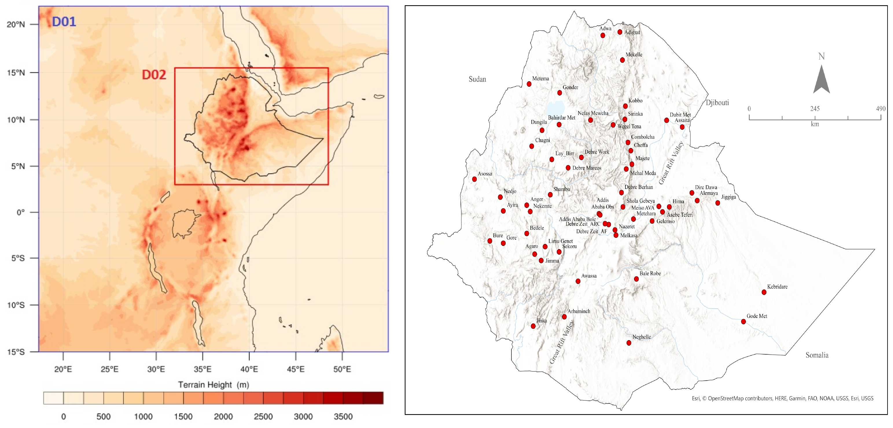
2.1. Verification Data

In order to address uncertainties associated with observations, three different datasets were used to evaluate the performance of WRF simulations: daily precipitation from 57 meteorological stations obtained from the National Meteorology Institute (NMI) of Ethiopia archive (Figure 1); gridded monthly precipitation from the Climate Hazards Infrared Precipitation with Stations version 2 (CHIRPS [29]); and the gauge-satellite blended rainfall estimate from the Enhancing National Climate Services initiative (ENACTS [30,31]). The CHIRPS dataset has a resolution of 0.05${ }^{\circ }$× 0.05${ }^{\circ }$ while ENACT has around a 0.1${ }^{\circ }$× 0.1${ }^{\circ }$ (∼≈ 10 km) resolution; they were mainly used to evaluate performance in terms of capturing the magnitude and spatial distribution of mean seasonal precipitation. To facilitate grid-to-grid comparison with WRF simulations, both the CHIRPS and ENACTS datasets were regridded from their native grid to the WRF simulation grid configuration using a bilinear interpolation routine from the Earth System Modeling Framework (ESMF) in NCAR Command Language (NCL) version 6.3 [32].

Despite having comparable spatial resolution to WRF simulations, the datasets exhibited lower spatial details in rainfall compared to WRF simulations, likely owing to the sparse network of weather stations used in developing these datasets. Thus, it is important to note the possible uncertainties this mismatch could impose when using these datasets to verify WRF simulations. However, even though these datasets are relatively the best available products over the region ([33,34]) and the station network over the area is sparse and uneven, they have been utilized for the evaluation. In addition, evaluation of performance related to intensity and frequency of rainfall events was performed with respect to weather stations only, as the gridded products lack data or are unreliable on daily time scales. For evaluations involving weather stations, data for WRF grid points nearest to respective stations were extracted.

2.2. Initial and Boundary Conditions

The initial and lateral boundary conditions (including SST) used to drive WRF were extracted from the Climate Forecast System Reanalysis (CFSR) dataset [35]. The CFSR surface variables have a 0.312${ }^{\circ }$× 0.312${ }^{\circ }$ resolution while pressure level data have a 0.5${ }^{\circ }$× 0.5${ }^{\circ }$ resolution, with the model top at 1 mb. These datasets (i.e., temperature, humidity, surface pressure, geopotential heights, and wind) were prescribed at 6 h intervals starting on May 1st and were obtained from the NCAR Research Data Archive [36].

2.3. Model Set Up: Domain and Integration Time

We used a two-domain configuration with one-way nesting for all simulations: parent domain (D01) and nested domain (D02), with resolutions of 12 km and 4 km, respectively (Figure 1). The parent domain (D01) was centered on Ethiopia, extending from 15${ }^{\circ }$ S to 22${ }^{\circ }$ N and 15${ }^{\circ }$ E to 55${ }^{\circ }$ E, encompassing the entire Greater Horn of Africa, central Africa, parts of southern Africa, Red Sea, parts of North Africa and the Middle East, Arabian Sea, and the western half of the Indian Ocean. The placement was intended to encompass, to the extent feasible, regions that include synoptic features and circulations which directly influence the summer climate over Ethiopia. Although the domain is not large enough to incorporate synoptic systems starting from their source regions (e.g., low-level flow from Atlantic Ocean to Ethiopia begins from the southern Atlantic ocean where the St. Helena high is located), findings from previous studies (e.g., [11,37]) suggest that the domain is large enough for systems to develop fully. For example, Ref. [11] carried out a sensitivity experiment using RegCM3 driven by an ECMWF seasonal hindcast to quantify the impact of domain size in simulating the spatial patterns of summer rainfall over Ethiopia using a two-domain setup, one covering the horn of Africa (23${ }^{\circ }$ E to 57${ }^{\circ }$ E, 5${ }^{\circ }$ S to 23${ }^{\circ }$ N) and the second smaller domain covering only Ethiopia. They found that the larger domain was far better in reproducing the observed summer rainfall pattern while the smaller domain performed relatively poorly to the extent that the location of rainfall maxima was misplaced. The above study, while showing the importance of domain size in simulating summer precipitation over Ethiopia, also partly justifies that the size of the outer domain used in our study (which extends further south and west by 10 degrees compared to the larger domain used in [11]) was sufficiently large not to be too constrained to reproduce errors in the driving reanalysis [17]. The nested domain (D02) on the other hand covers the whole of Ethiopia with a few extra grid cells on all sides to account for a relaxation zone. The results discussed in subsequent sections will be based on simulation outputs from D02.

As for the horizontal resolution, a uniform vertical resolution of 40 eta levels spaced closer together in the PBL were used across all simulations. The vertical level covered the whole troposphere, with the resolution decreasing slowly with height to allow low-level flow details to be captured. The first 20 levels are inside the atmospheric boundary layer (below 1500 m), with the first level at approximately 16 m, and the domain top at 100 hPa. Although it is recognized that the choice of model horizontal and vertical resolution, the size and location of domain boundary, and the choice of boundary conditions can be equally important for the choice of physics options (e.g., [17,28]), identifying the optimum configuration for these options was beyond the scope of this study. This sensitivity experiment was conducted for the anomalously dry summer season of 2002, with each simulation covering the period from May 1st to August 31st. The first month of the simulation (i.e., May) was considered as model spin-up and only the simulations from June through August were used for model evaluation.

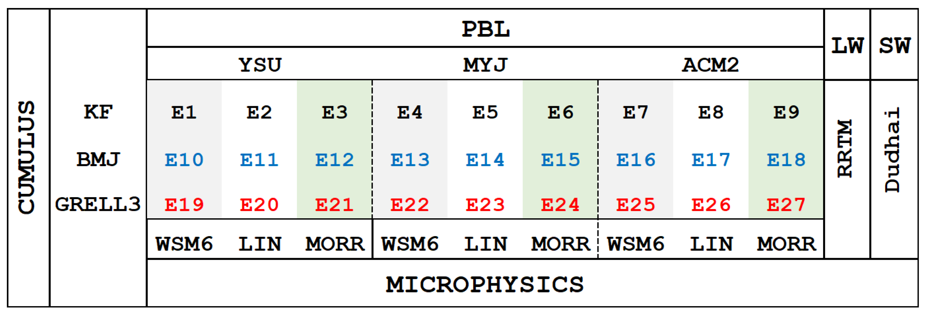
2.4. Experimental Setup

The WRF model comprises multiple options for most parameterization schemes that can be combined in any different way, enabling the user to optimize the model for a range of spatial and temporal resolutions and climatologically different geographical regions [21]. The options typically range from simple and efficient to sophisticated and more computationally costly, and from newly developed schemes to well-tried schemes such as those in current operational models. The accuracy of a WRF configured with a certain scheme cannot be uniquely attributed to a single parameterization but rather to the combination of them, since feedbacks are usually as important as the schemes themselves [38]. Furthermore, the suitability of a specific configuration strongly depends on the region, the season, or even the particular event considered, and hence, there is no single configuration appropriate for every situation. Thus, testing as many combinations of parameterization schemes as possible would be beneficial to identify an optimum configuration. However, since testing all possible combinations of parameterization schemes was not feasible, we considered a small subset based on the most commonly used schemes for selected physics options.

Figure 2 shows the parameterization schemes tested and how the different physics options for each were combined. The cumulus parameterization (CU) is the scheme with the highest impact on precipitation simulation and is used to predict the collective effects of convective clouds at smaller scales as a function of larger-scale processes and conditions. The options tested were Kain–Fritsch (KF [39]), Betts–Miller–Janjic (BMJ [40,41]) and Grell 3D (Grell [42,43]). It should be noted that the CU schemes were uniformly applied to both the outer and nested domains in all of our simulations. While there is a growing consensus that CU parametrization may not be necessary at resolutions such as 4 km to explicitly resolve convection, our preliminary tests conducted at this scale, both with and without CU parameterization showed no significant improvement and, in some cases, even deterioration in model performance when CU was omitted. These findings align with those reported by [16,44], suggesting that the exclusion of CU parameterization under the complex meteorological conditions of our study area does not notably benefit the simulation outcomes. Consequently, experiments without CU parameterization were not included in the sensitivity study. The planetary boundary layer (PBL) and surface layer schemes define boundary layer fluxes (heat, moisture, momentum) and the vertical diffusion processes. For the PBL (and surface layer) the Yonsei University (YSU [45]), Mellor–Yamada–Janjic scheme (MYJ [40]), and Asymmetric Convective Model (ACM2 [46]) were tested. In the WRF model, some PBL schemes are tied to particular surface layer schemes [19], so a single common surface layer scheme could not be used here. Thus, the Revised MM5 Monin–Obukhov scheme ([47]) was used with YSU and ACM2, and the Monin–Obukhov (Janjic Eta) scheme [48] was used with the MYJ scheme. The microphysics (MP) schemes allow the prediction of water phase transitions in the atmosphere and for consideration of snow and hail. The MP options tested were the WRF Single-Moment 6-class (WSM6 [49]), and the LIN [50] and Morrison double-moment scheme (MOR [51]). The combination of 3 options from CU, PBL, and MP resulted in 27 simulations with longwave (LW) and shortwave radiation (SW) parameterizations set to the Rapid Radiative Transfer Model (RRTM [52]) and Dudhia shortwave scheme (Dudhai [53]), respectively. In addition to the 27 simulations above, 3 more simulations were performed to test the sensitivity to the selection of radiation schemes where the RRTMG shortwave and longwave scheme (RRTMG [54]) was combined with Dudhia and RRTM schemes (

Table 1. Additional set of experiments for radiation parameterization sensitivity.

WRF Run	CU	PBL	MP	LW	SW
E28	KF	YSU	WSM6	RRTMG	Dudhia
E29	KF	YSU	WSM6	RRTM	RRTMG
E30	KF	YSU	WSM6	RRTMG	RRTMG
E31	KF	MYJ	LIN	RRTMG	RRTMG
E32	KF	MYJ	MOR	RRTMG	RRTMG
E33	KF	MYJ	WSM6	RRTMG	RRTMG
E34	KF	MYJ	LIN	RRTMG	RRTMG
E35	KF	MYJ	MOR	RRTMG	RRTMG

). Unlike the RRTM/Dudhia schemes that consider a binary measure of grid cloudiness, the RRTMG scheme uses overlapping cloud fraction algorithms to determine the cloudiness of the grid. Furthermore, the RRTMG scheme takes into account the concentrations of trace gases, aerosols, ozone, and carbon dioxide, and considers reflected shortwave radiation fluxes [25]. All the 35 experiments used the Noah land surface model [55], and MODIS 21-class land use data.

Due to the scarcity of region-specific WRF sensitivity studies for Ethiopia, the selection of options tested for each physics parameterization was primarily guided by their widespread adoption across diverse meteorological settings, which serves as a proxy for their effectiveness and adaptability. Consequently, we referred to the ‘WRF Physics Use Survey’ to identify the top two or three most favored schemes based on their frequency of use by the global WRF community [56]. Furthermore, a review of the limited regional climate modeling studies within the region (e.g., [8,9,28,57,58,59]) revealed that the schemes tested in this sensitivity study are among the most commonly utilized options. Although some of these studies did not directly compare scheme performances, they provided valuable insights into their practical applications.

2.5. Evaluation Statistics

The WRF-simulated and observed precipitation values from meteorological stations, as well as gridded precipitation products, are compared using four different statistics: the mean absolute error with respect to weather stations and gridded data (MAE_stn and MAE_grd), the pattern correlation coefficient (PCC), the Pearson correlation coefficient (R), and the daily intensity index and frequency of rainy days in the season. The gridded rainfall products (i.e., CHIRPS and ENACT) were used as observational references in calculating the first two statistics only, while daily rainfall from weather stations was used to calculate all but PCC. The MAE was used to measure the closeness of the modeled and observed values. For grid-based comparison, mean JJA rainfall was first computed for observations and WRF simulations and MAE was calculated over each grid-point pair with respect to both gridded datasets. For station-based comparison, absolute value of bias was calculated for each day and averaged over 92 days in the season. The PCC was computed from observed and simulated mean JJA rainfall (Equation (1)) according to the usual Pearson correlation operating on the M grid-point pairs from WRF and the gridded observations [60].

$$PCC={\displaystyle \frac{{\displaystyle \sum _{m=1}^M}(y_m-\overline{y})(o_m-\overline{o})}{{\left[{\displaystyle \sum _{m=1}^M}{(y_m-\overline{y})}^2{\displaystyle \sum _{m=1}^M}{(o_m-\overline{o})}^2\right]}^{1/2}}}$$

(1)

where $y\left(o\right)$ is WRF-simulated (observed) seasonal mean precipitation at the mth grid point and the over-bars refer to these variables averaged over M grid points (i.e., here, M refers to grid points within the boundary of Ethiopia). The PCC ranges from −1 to 1, with values closer to one indicating a higher skill of WRF in capturing the observed spatial patterns of mean seasonal precipitation over Ethiopia. The PCC was calculated with respect to both CHIRPS and ENACT and values reported here are averages of the two. The correlation coefficient (R) was used to quantify the ability of WRF simulations in reproducing the intra-seasonal variation of daily precipitation and was calculated from time series of daily precipitation from 1st June to 31st August 2002 between gauging stations and WRF grid points where the respective stations fall. The error in frequency of rainy days (ERD) was computed as the difference between simulated and observed (gauging stations) total number of rainy days (i.e., daily precipitation greater than 1 mm). Similarly, the mean daily intensity was compared by dividing the total precipitation in the season with the total number of rainy days in the season.

In order to rank the different combinations of physics options based on performance statistics, a new aggregate score (AS) was computed. As the above statistics have different units, range, and orientation, simple manipulations were applied to the scores before aggregation. First, evaluation metrics that were computed over multiple grid points or stations (i.e., all except PCC) were averaged (spatially) to create one score for each experiment. In terms of score orientation, R and PCC are positively oriented (larger value indicating higher performance) while MAE, MB, and ERD are negatively oriented. To facilitate aggregation, R and PCC were converted to negative orientation by subtracting the scores from 1 (1-R or 1-PCC). All statistical scores were then normalized using Equation (2) [61] to change their range to 0 to 1.

$$X_{norm}={\displaystyle \frac{X_i-X_{min}}{X_{max}-X_{min}}}$$

(2)

where X is a score and X${ }_{min}$ and X${ }_{max}$ are defined by the best and worst of the 27 simulations for any given score. Thereafter, the aggregate scores (ASs) were computed as the sum of the normalized (X_norm) values of R, PCC, MAE_stn, MAE_grd, and ERD (Equation (3)), as in [61]. As each of the five normalized terms has values ranging from 0 (for the best) to 1 (for the worst), the AS has a range between 0 (best) and 5 (worst).

$$AS=R_{norm}+PC{C}_{norm}+MA{E}_{norm\left(stn\right)}+MA{E}_{norm\left(grd\right)}+ER{D}_{norm}$$

(3)

3. Results and Discussion

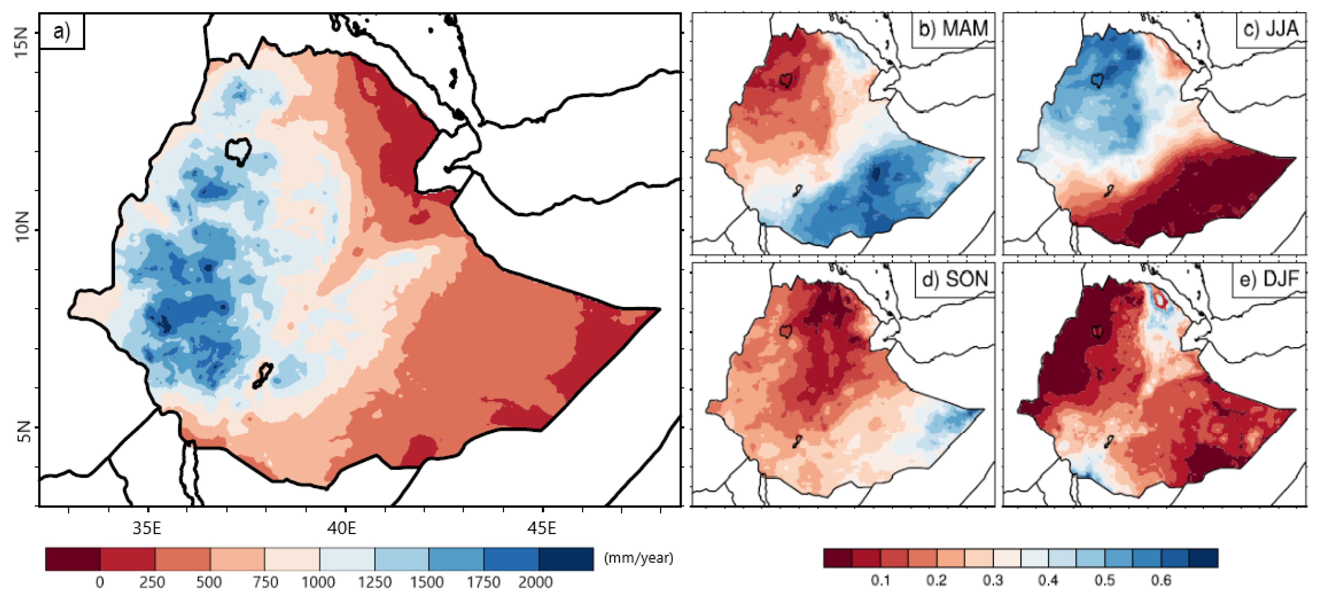
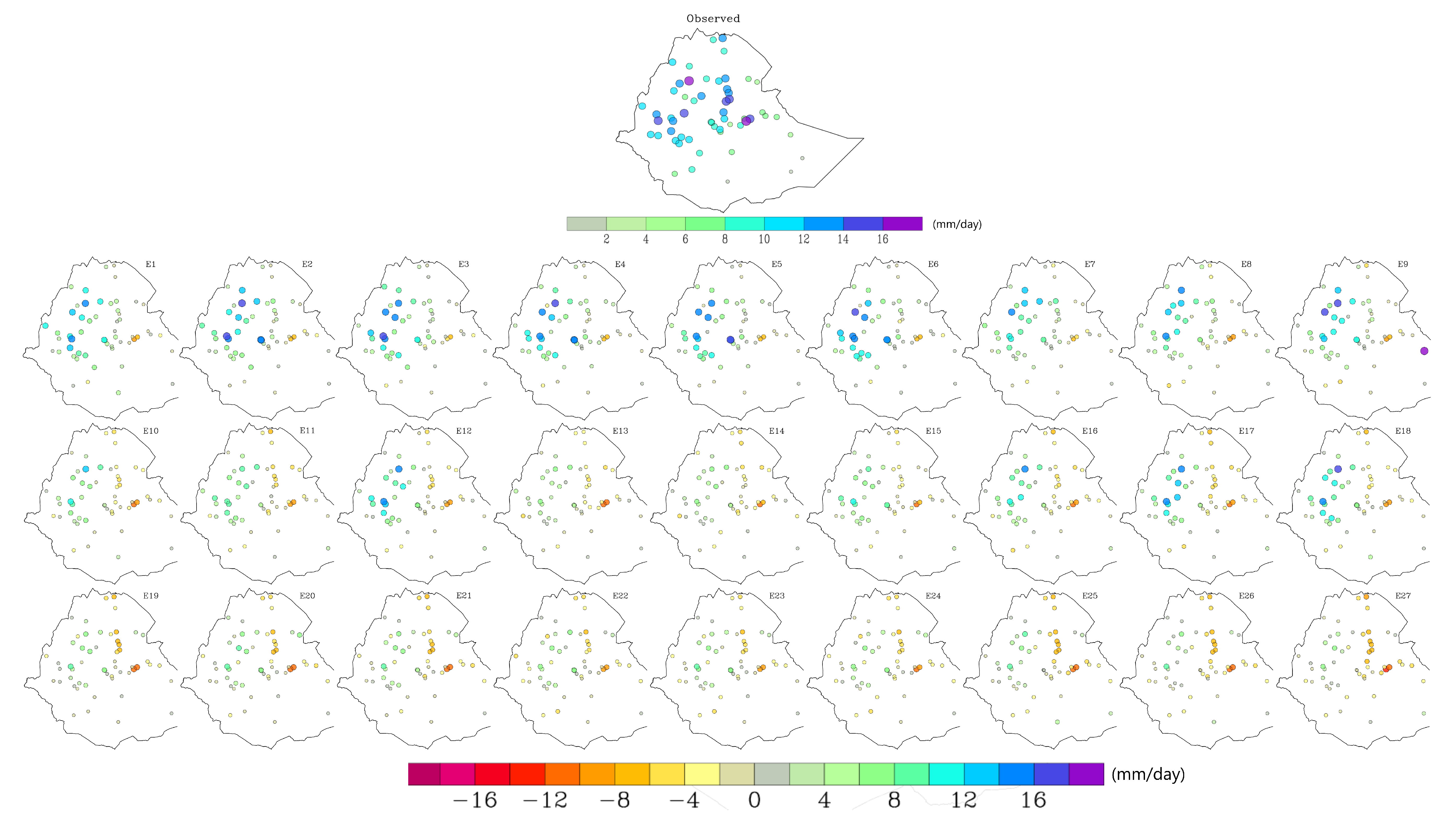
3.1. Mean Seasonal Precipitation

Based on the analysis of long-term rainfall records from CHIRPS and ENACTS, the northwestern, western, and central regions of Ethiopia (where summer is the main rainy season) receive on average more than 12 mm day⁻¹ of rainfall. The semi-arid regions of northeastern, eastern, southeastern, and southern Ethiopia on the other hand receive comparably less rainfall during the JJA season, accounting for less than 35% of the annual rainfall (Figure A1). The observed mean JJA rainfall in 2002 from the CHIRPS and ENACTS datasets is shown in Figure 3a and Figure 3b, respectively. As expected, the summer-rain receiving areas in western/northwestern Ethiopia received a higher amount of rainfall, up to 15 mm/day. The ENACTS dataset showed a slightly wetter summer, with patches as high as 21 mm day⁻¹ of rainfall. All 27 WRF simulations reproduced the observed spatial patterns of JJA rainfall (e.g., the north–south and east–west rainfall gradients, rainfall gradient within and on either side of Central Rift Valley, and fine-scale patterns associated with topography (Figure A1)). This was evident from the high PCC scores, ranging from 0.92 to 0.96 when compared with CHIRPS (Figure 4a) and 0.86 to 0.93 when compared with ENACTS (Figure 4b). However, despite reproducing spatial patterns of rainfall, all simulations consistently overestimated JJA rainfall, with prominent wet bias over the Ethiopian highlands (i.e., western, and northwestern Ethiopia, and the Bale Mountains on the eastern side of the Rift Valley) and to a lesser extent over the northeastern lowlands. In terms of dry bias, the southwestern and eastern parts of the country were locations where simulations consistently underestimated JJA rainfall. However, the magnitudes of the dry bias were significantly smaller than the wet bias (<4 mm day⁻¹). Ref. [62] also found a similar pattern in JJA rainfall climatology, where Regional Climate Model version 4 (RegCM4), despite reproducing spatial rainfall patterns, showed positive (negative) biases over the highlands in western Ethiopia (isolated lowland areas).

The wet bias was the highest for simulations using the KF CU followed by the BMJ CU scheme (Figure 3 and Figure A2). For the simulation using the KF CU, extreme wet bias as high as 20 mm day⁻¹ day can be seen covering a significant area in western and northwestern Ethiopia, and highlands east of the Central Rift Valley. For most of these areas, this magnitude of wet bias is more than 150% of the observed rainfall. The wet bias over the northeastern lowlands was smaller in magnitude compared to the highlands (<10 mm day⁻¹). However, given this location received less than 6 mm/day (mostly <3 mm day⁻¹), the bias translates into more than 150% of the observed JJA rainfall. For BMJ CU, the spatial extent of bias magnitudes on the order of 20 mm/day was significantly reduced to localized areas. However, wet bias of 4–10 mm day⁻¹ covering a significant area in the highlands still exists. The spatial pattern of bias in BMJ CU was mostly similar to KF CU, except over the northeast where the wet bias in KF CU (as well as Grell CU) switched to dry bias in BMJ CU. The differences in wet bias magnitudes between the KF and BMJ CU schemes are in line with those of [28,59], who also found KF to simulate a wetter climate than the BMJ scheme for Equatorial East Africa and the Nile River Basin, respectively. For Grell CU, wet bias magnitudes above 12 mm day⁻¹ were limited to a few small patches, and wet bias over similar locations as the KF and BMJ schemes were below 10 mm day⁻¹. However, wet bias over the northeast was more severe than KF, especially when used with the YSU and MYJ PBL schemes. Unlike KF CU, Grell CU simulations had a dry bias of up to 4 mm day⁻¹ over a narrow strip stretching from north-central to central Ethiopia. This dry bias was more pronounced when Grell CU was used with ACM2 PBL. This long stretching area of dry bias is characterized by a sharp transition in altitude from the northeastern lowlands with an altitude of below 250 m to highlands in the west with altitudes above 3000 m (Figure 1). The above wet bias pattern was to some extent observed in the BMJ CU scheme. The large wet bias over highlands of Ethiopia is in line with previous studies [57,63]. For example, Ref. [57] evaluated the ability of several RCMs in the CORDEX experiment to simulate the rainfall patterns over East Africa and found WRF to overestimate JJA rainfall climatology over the Ethiopian highlands. Although the horizontal resolution of 50 km used in [57] was coarser than this study, the model setup was fairly similar to E1 (KF CU, YSU PBL, and WSM6 MP schemes) of this study.

The wet bias for simulations with the KF CU scheme showed no significant difference when used with either the YSU or MYJ PBL schemes (Figure A2). This contrasts with findings from [59], who reported less biased rainfall when KF CU was combined with MYJ compared to YSU for the Nile River Basin. It is important to consider the differences in simulation setups that might contribute to these divergent results, such as our use of a finer resolution of 4 km compared to their 36 km for nested domain, and our specific focus on seasonal rather than annual rainfall patterns. However, in our configurations, KF showed improved performance when used with the ACM2 PBL scheme, particularly with significant reductions in wet bias over the highlands in west/northwest (up to 14 mm day⁻¹) and over the lowlands in the northeast (up to 6 mm day⁻¹). On the contrary, areas in the western and southwestern peripheries of the country became relatively drier when KF CU was used with ACM2 PBL. A similar dry bias pattern was also observed when the BMJ and Grell CU schemes were used with the ACM2 PBL scheme. There was no notable difference in bias when KF CU was used with any of the three MP schemes. When the KF and Grell CU schemes were used with the MYJ PBL scheme, there was a notable increase in wet bias over the northeastern lowlands. For the KF CU scheme, the wet bias increased in magnitude and extended further east when used with the MYJ PBL scheme. For the Grell CU scheme, the wet bias was present across all simulations, but the magnitude increased when used with the MYJ scheme. Unlike KF and Grell, the BMJ CU scheme performed better when used with the MYJ PBL scheme, with significantly smaller wet bias over the highlands and better representation of the precipitation gradient on either side of the Rift Valley. This is in line with the findings of [61] who pointed out that schemes that are developed together tend to perform better. The JJA rainfall was least sensitive to MP schemes. The increased magnitude of wet bias over west/northwest when the BMJ CU and YSU PBL schemes were used with the Morrison MP scheme was the only noticeable change in JJA rainfall compared to the WSM6 and LIN MP schemes.

The systematic overestimation of JJA rainfall observed across all simulations can be partly attributed to over-sensitivity to topography, as evidenced by the exaggerated details in WRF simulations when compared to the CHIRPS and ENACTS datasets, that have a comparable resolution to the WRF simulations. This phenomenon is particularly pronounced in regions characterized by complex terrain, such as the Ethiopian highlands [64]. Ref. [11] found a similar result in a dynamical downscaling study over East Africa using Regional Climate Model version 3 (RegCM3) and suggested misrepresented topographic forcing and the diagnostic nature of convective parametrization schemes that prevent advection of evolving convective systems from one grid cell to another as potential reasons [65].

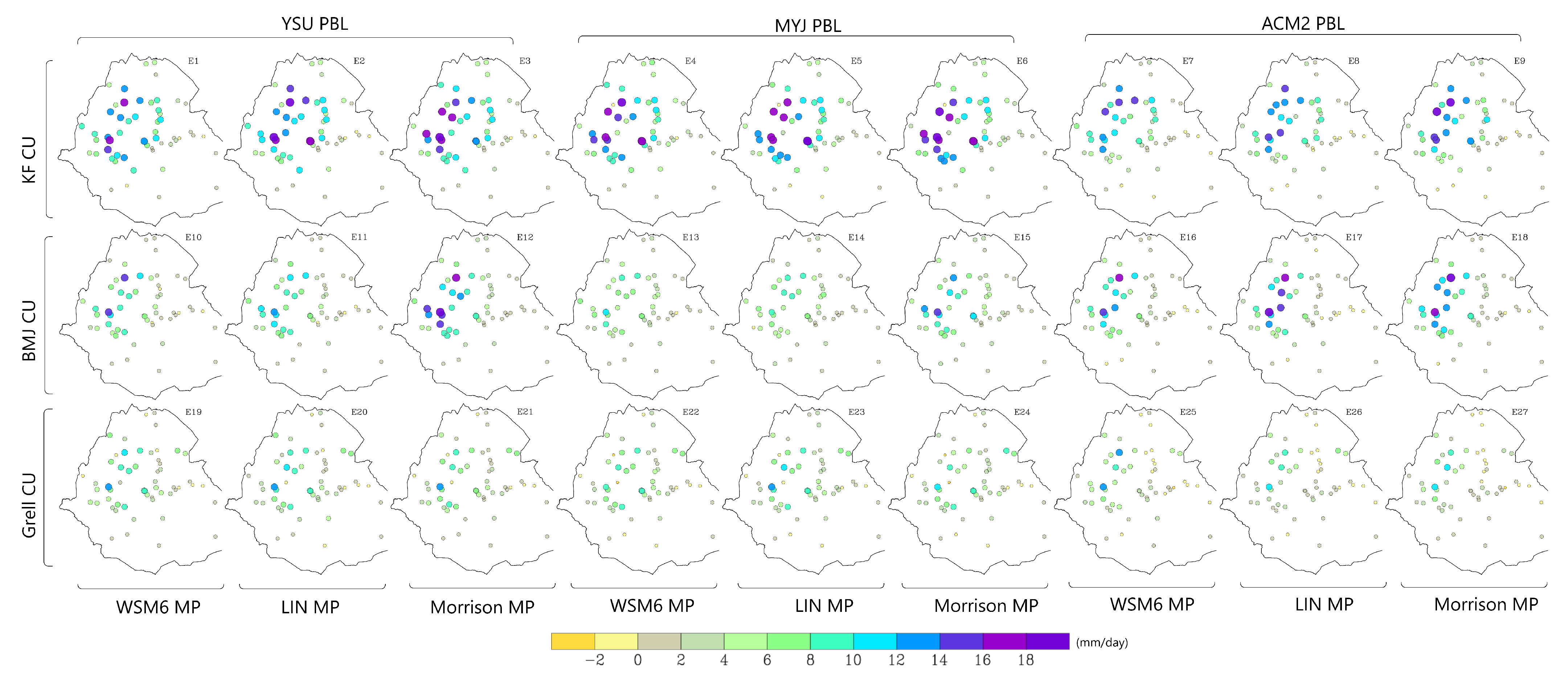
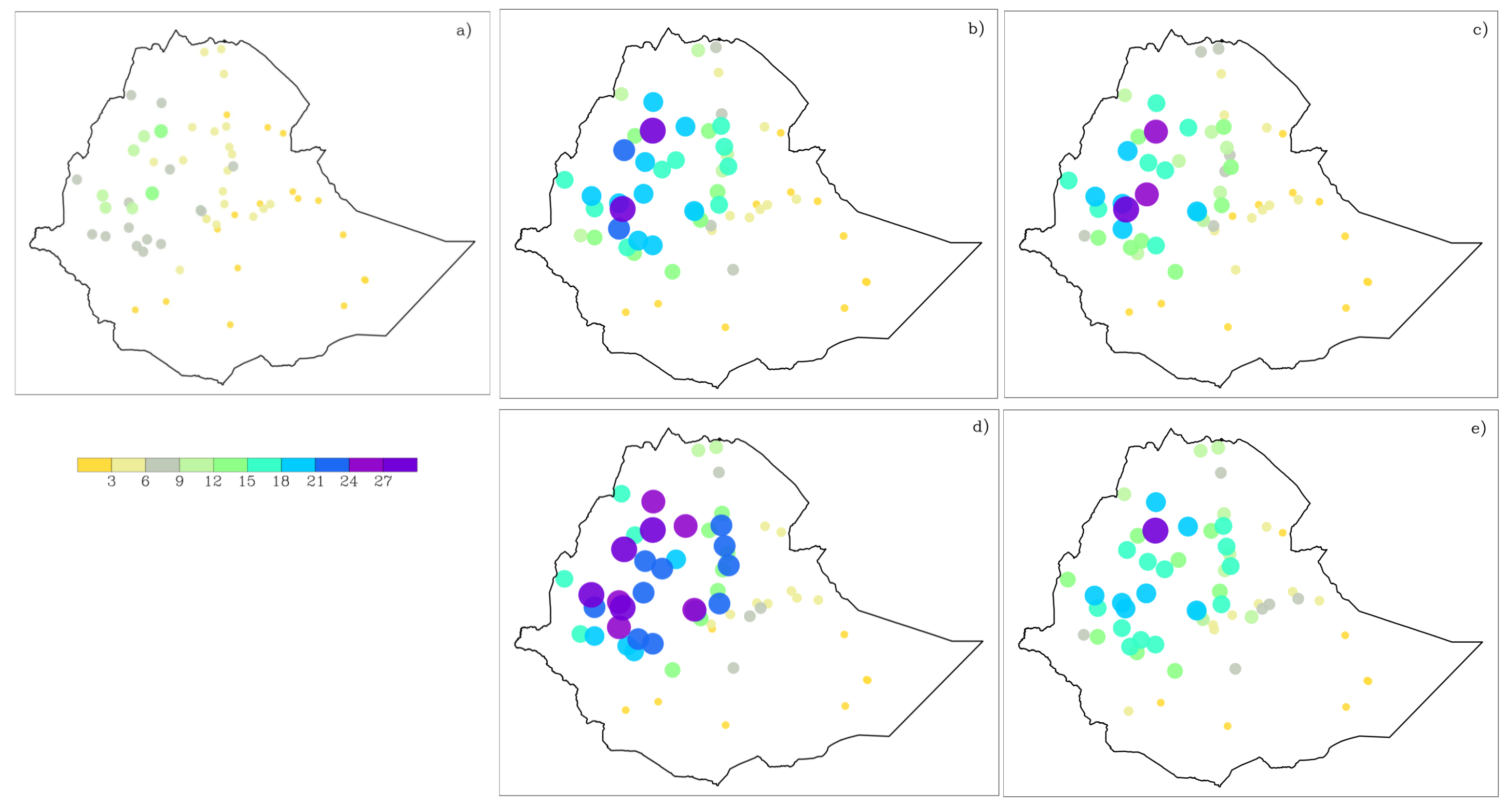
3.2. Rainy Day Frequency and Intensity

The WRF simulations were evaluated for their performance in reproducing the observed frequency of rainy days and the various categories of rainfall intensities over the 92 day simulation period. The observed rainy day frequency (Figure 5, top) showed large spatial variability, ranging from 0 days in the southern and southeastern lowlands, where JJA is not the main rainy season (e.g., 0, 0, 2, and 3 days over Kebridehar, Gode, Negelle, and Degehabour stations; see Figure 1 for location of stations), to more than 75 days over stations located in the western and northwestern highlands (e.g., Bahirdar, Debremarkos, Chagni, Nekemte, and Shambu). The significantly larger number of rainy days over western and northwestern Ethiopia was however expected as these locations receive a larger share of annual rainfall during the summer months. Overall, all the WRF simulations overestimated rainy days except for four stations in the south and southeast (i.e., Arba Minch, Negelle, Jijiga, and Degehabour) that underestimated the number of rainy days by 1 to 6 days for selected experiments. However, the above cases account for only 1.3% of the total station–experiment combinations (i.e., 20 cases out of 1512). Out of the 20 cases, 55% occurred at Negelle station, located in southern Ethiopia, and 50% (40%) of the 20 experiments used the KF (Grell) CU scheme.

Unlike the few cases of underestimated rainy days, the magnitude of positive bias was significantly larger and exceeded 65 days over the arid northeastern lowlands for simulations using the Grell CU scheme. As seen in Figure 5, rainy day bias followed a similar spatial pattern across experiments. The most prominent pattern was the relatively higher bias magnitudes at stations located around the western (stretching from north to central Ethiopia) and eastern escarpments of the Rift Valley (stretching from south to east following mountain ranges). This was contrary to the significantly fewer observed rainy days at these stations (<45 days) compared to those in western and northwestern parts of the country (Figure 5, top). The other consistent patterns were the lowest (highest) magnitude of bias at stations located in the southern and southeastern (northeastern) lowlands which had observed rainy day frequencies of less than 15 days.

In general, all simulations involving the Grell CU scheme (E19–E27) showed a higher bias compared to corresponding experiments utilizing the KF and BMJ CU schemes (

Table 2. Summary statistics for rainy day frequency averaged over parameterization options and weather stations.

Physics Option	Parameterization Scheme	Mean Bias	Mean Bias (ACM2-Only)	Bias Range
	KF	24.8	18.2	16.6–30.8
CU	BMJ	26.3	21.1	18.8–31.0
	Grell	31.1	25.8	25.4–35.6
	YSU	28.9	-	25.7–32.7
PBL	MYJ	31.6	-	28.4–35.6
	ACM2	21.7	-	16.6–26.0
	WSM6	27.0	21.0	17.3–35.0
MP	LIN	27.0	20.3	16.6–35.6
	MOR	28.3	23.8	20.8–34.7

). When averaged over all stations and experiments, rainy days bias for the nine Grell-only experiments had a bias of around 31.1 days while KF-only and BMJ-only simulations showed 24.8 and 26.3 days, respectively. The higher bias in rainy day frequency observed with the Grell scheme suggests its convective triggering mechanism might be too sensitive for the complex terrain of Ethiopia, potentially exacerbating frequency bias, as noted in similar studies [66]. The rainy day frequency was most sensitive to the selection of PBL schemes, with bias ranging from 21.6 days for ACM2-only experiments to 31.6 days for MYJ-only experiments. On the other hand, rainy day frequency was least sensitive to MP schemes, with only 1 day difference between MP schemes (Table 2). In general, all the CU and MP schemes performed better when used together with ACM2 PBL scheme. For example, the average bias increased from 18.2 days when KF CU (E7–E9) was used with ACM2 PBL to 25.9 and 30.3 days when KF CU was used with YSU PBL (E1–E3) and MYJ PBL (E4–E6), respectively. A similar difference was observed when bias was averaged over the PBL schemes (regardless of CU and MP options), where ACM2-only experiments (E7–E9, E16–E18, E25–E27) had a significantly lower bias (i.e., 21.7 days) compared to YSU-only (E1–E3, E10–E12, E19–E21; 28.9 days) and MYJ-only experiments (E4–E6, E13–E14, E22–E24; 31.6 days). In addition, out of the nine experiments with the least bias averaged over stations, seven used the ACM2 PBL scheme. When considering frequency of rainy days as an evaluation criteria, the above results suggest that simulation E8 (KF CU, ACM2 PBL, and LIN MP) followed by E7 (KF CU, ACM2 PBL, and Morrison MP) performed relatively better (Figure 5, Table 2 and

Table A1. Summary statistics for rainy day bias for 27 experiments averaged over 57 stations.

No. of Stations in Each Bias Category								Max. Bias (Days)	Avg. Bias (Days)
ID	0–10	10–20	20–30	30–40	40–50	50–60	60–70
E1	5	12	13	10	7	0	0	46	22.9
E2	6	13	15	7	9	0	0	47	23.7
E3	4	17	10	10	8	0	0	46	22.7
E4	4	10	10	8	10	3	0	53	26.7
E5	4	9	12	7	13	1	0	52	27.3
E6	5	12	12	6	11	3	0	54	26.9
E7	12	19	11	6	1	0	0	44	16
E8	13	14	13	5	1	0	0	42	15.5
E9	7	15	14	8	2	0	0	44	18.9
E10	3	14	12	14	4	1	0	53	25.6
E11	4	13	14	17	3	1	0	52	26.1
E12	5	9	18	14	4	2	0	56	27.1
E13	4	12	19	10	6	2	0	52	27.1
E14	4	9	15	16	5	2	0	53	27.8
E15	3	12	13	11	8	2	0	56	29.2
E16	6	18	17	6	2	0	0	47	19.3
E17	10	15	18	5	2	0	0	43	18.8
E18	6	14	16	12	4	0	0	47	23.7
E19	6	7	10	14	8	5	1	62	29.2
E20	4	9	10	14	9	4	0	59	29.2
E21	4	10	9	12	10	3	1	61	29.4
E22	3	10	10	8	12	4	2	68	30.9
E23	3	7	11	8	11	5	2	65	31.3
E24	4	9	11	10	11	4	2	69	30.9
E25	7	9	16	13	5	2	0	56	25.4
E26	3	14	12	14	6	2	0	56	25.3
E27	4	13	14	14	4	3	0	60	26.6

).

In terms of daily rainfall intensity, simulations showed a general spatial pattern where intensity was overestimated over the highlands (i.e., central, western, and northwestern Ethiopia) and either slightly overestimated or underestimated elsewhere (Figure 6). This pattern was a reverse of the bias in the rainy day frequency, where areas with larger (smaller) rainy day bias had a smaller (larger) bias in rainfall intensity. As for mean seasonal rainfall, intensity showed the most sensitivity to the selection of CU parameterization options followed by PBL, and MP options. For example, mean absolute bias (MAB) in rainfall intensity for experiments using KF CU (E1–E9) changed by a maximum of 1 mm day^$-1$ when changing PBL and MP options. On the other hand, changing KF CU to BMJ CU (E10–E18) or Grell CU (E19–E27) resulted in up to 2 mm day^$-1$ change in MAB in intensity (

Table A2. Summary statistics for rainfall intensity bias for 27 experiments averaged over 57 stations.

Exp. ID	Mean Bias (mm)			MAB (mm)	No. of Stations		MAB/Option
	Avg.	Min.	Max.		MAB < 5	MAB > 10
E1	4.1	−8.3	15.1	5.2	24	10	KF-only = 5.0
E2	4.1	−8	17.1	5.4	24	10	BMJ-only = 4.0
E3	4.3	−7	16.5	5.4	24	9	Grell-only = 3.4
E4	4	−8	17.3	5.2	22	11	YSU-only = 4.3
E5	4	−7.6	16.8	5.1	23	9	MYJ-only = 3.9
E6	4.2	−7.3	17.5	5.3	22	13	ACM2-only = 4.2
E7	3.2	−7.6	14.7	4.4	21	6	WSM6-only = 4.1
E8	2.9	−8.3	15.5	4.7	20	6	LIN-only = 4.1
E9	3.1	−8.9	17.9	4.6	18	10	MOR-only = 4.3
E10	0.6	−10.4	12	3.8	16	3
E11	0.8	−9.9	9.4	4.2	18	0
E12	2	−9.9	15	4.5	21	6
E13	0.2	−11	7.1	3.1	10	2
E14	0	−10.7	6.9	3	10	1
E15	1.2	−10.1	10.9	3.5	14	2
E16	1.1	−10.2	14.8	4.4	17	4
E17	1.1	−11.6	15.7	4.8	18	6
E18	1.9	−9.5	17.9	4.8	22	6
E19	−0.2	−10.2	8.9	3.4	18	2
E20	−0.3	−10.3	9.4	3.6	18	2
E21	−0.6	−11.3	8.2	3.6	19	2
E22	−0.6	−9.8	7.6	3.3	14	0
E23	−0.4	−9.3	8.8	3.2	13	0
E24	−0.9	−10.1	6.9	3.3	12	1
E25	−1	−11.7	9.6	3.7	13	2
E26	−1.8	−11.7	8.1	3.3	14	2
E27	−1.8	−12.1	7.9	3.3	15	2

). This can also be seen from a summary of MAB (Table A2, last column) where MAB averaged over similar CU options has a relatively larger difference (1.6 mm) compared to differences in the PBL (0.4 mm) and MP (0.2 mm) parameterizations.

The ACM2 PBL scheme outperformed the YSU and MYJ schemes due to its hybrid approach that combines nonlocal transport driven by convective plumes with local eddy diffusion. This design allows ACM2 to effectively simulate both supergrid- and subgrid-scale turbulent transport in the convective boundary layer (CBL), enhancing the model’s ability to accurately predict the vertical transport of momentum, heat, and moisture, leading to more accurate simulation of both the frequency and intensity of rainfall [46]. In contrast, YSU focuses on large-scale upward-moving plumes through a nonlocal closure approach, which may not capture detailed localized mixing [45], while MYJ, employing a local closure based on turbulent kinetic energy (TKE), often under-represents the intensity of vertical mixing during strong convective updrafts [40]. The effectiveness of ACM2 in addressing the range of turbulent processes necessary for accurate precipitation modeling, particularly in complex terrains like the Ethiopian highlands, likely explains the observed reductions in bias when using this scheme. This effectiveness is corroborated by prior studies which have demonstrated similar improvements in model performance under convective conditions [67].

Comparison of the observed and simulated daily precipitation at selected stations further reveals the previously mentioned bias patterns in the frequency and intensity of rainy days (Figure 7). For instance, at Dangila station in northwestern Ethiopia (Figure 1 and Figure 7a) and Addis Ababa station in central Ethiopia (Figure 7b), simulations using the KF CU (blue line) and BMJ CU schemes (green line) exhibited a positive bias in both rainy day frequency and intensity, resulting in simulated precipitation consistently exceeding the observed daily amounts (black line). Simulations with the Grell scheme (red line) were relatively closer to observations due to the smaller magnitude of intensity bias. At Mekele station in northern Ethiopia (Figure 7c), a significant overestimation in rainy day frequency and underestimated intensity, particularly in simulations using the BMJ and Grell CU schemes, led to a persistent dry bias during rainfall events. Figure 7e further illustrates the poor performance of the Grell CU scheme in the dry northeastern lowlands, where the frequency of daily precipitation was severely overestimated and intensity underestimated. Additionally, the analysis at Dire Dawa station in eastern Ethiopia (Figure 7d) highlighted a distinct pattern within the region where simulation performance varied markedly throughout the season; for example, the bias in accurately simulating the occurrence or non-occurrence of rainfall events decreased from 11 days (9 days) in June and July to just 4 days in August. Further analysis of daily rainfall, using the correlation coefficient, revealed that simulations were generally most accurate in capturing the temporal variations of daily precipitation for stations located around the eastern escarpment of the Rift Valley in northern Ethiopia (Figure 8, G1), followed by eastern Ethiopia (Figure 8, G5). The least accurate performances were observed in southern and southwestern Ethiopia (Figure 8, G4 and G3), where summer does not constitute the primary rainy season. When comparing different experiments, simulations employing the BMJ and Grell CU schemes demonstrated superior capability in capturing these temporal variations compared to those using the KF CU scheme, particularly in central and eastern Ethiopia, where correlations were notably lower for KF CU simulations. Although less pronounced than with the cumulus schemes, simulations incorporating the ACM2 and YSU schemes outperformed those using the MYJ scheme. For instance, of the 18 cases (i.e., simulation–station combinations) with a correlation coefficient above 0.5, 14 utilized the ACM2 PBL scheme.

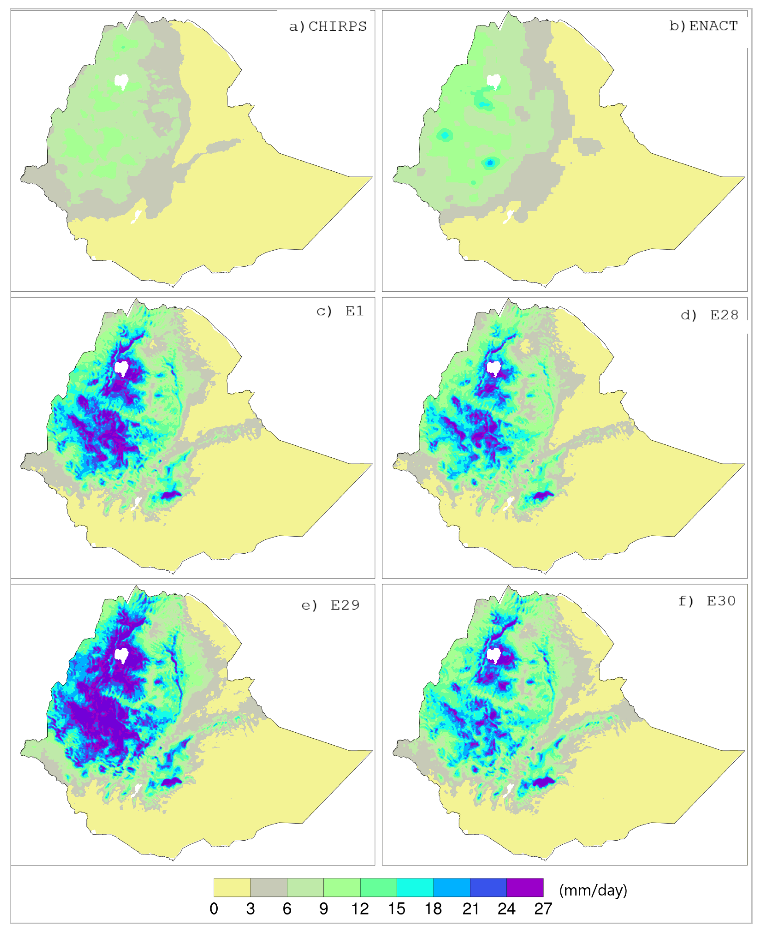
3.3. Radiation Schemes

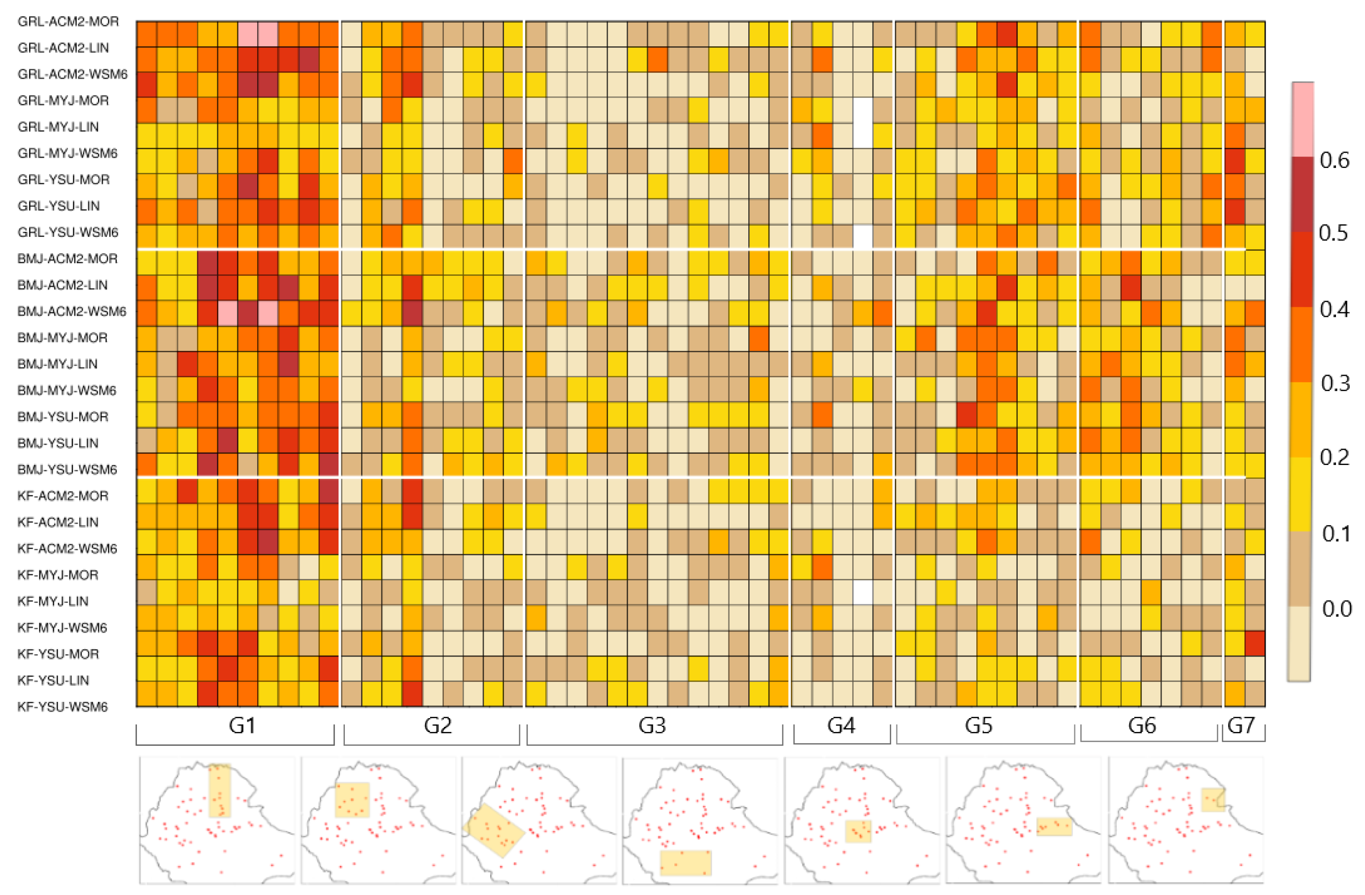
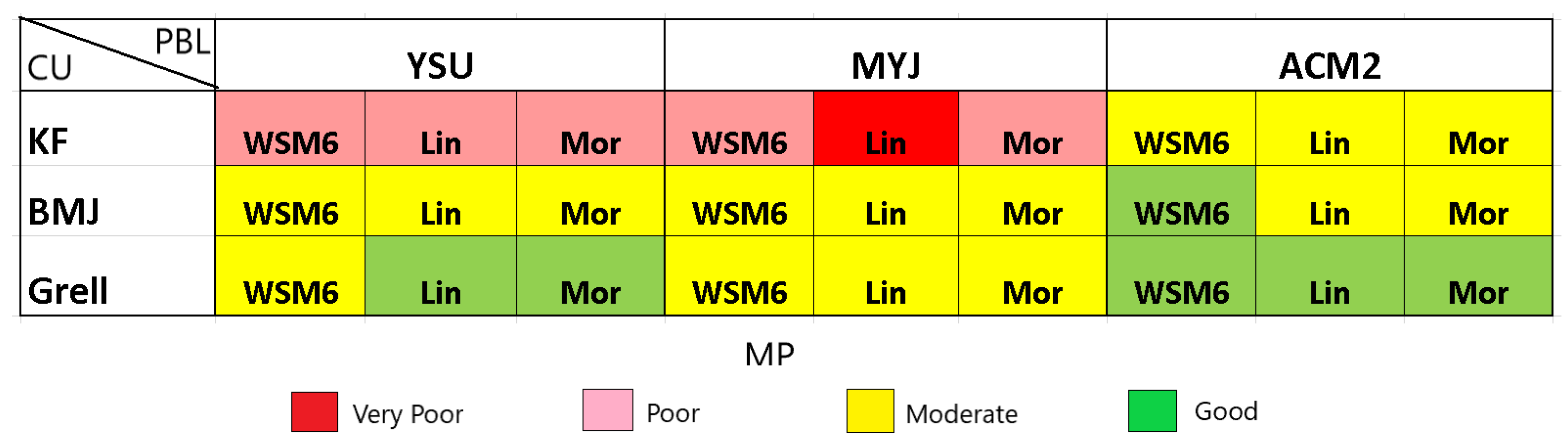
As stated in the methods section, assessing the sensitivity to radiation schemes (Table 1) was not part of the primary objectives of this study. Thus, the additional set of simulations (E28–E30) were run after completion of the 27 simulations that used fixed options for radiation parameterization (i.e., Dudhia for SW and RRTM for LW). These additional simulations were compared with E1, which used similar options for CU (i.e., KF), PBL (i.e., YSU), and MP (i.e., WSM6) as the three experiments. The LW (SW) schemes used in E1 were RRTM (Dudhai) while for E28, E29, and E30 they were RRTMG (Dudhai), RRTM (RRTMG), and RRTMG (RRTMG), respectively. Figure 9a–e shows a comparison of the mean JJA rainfall from the weather stations and radiation experiments E1, E28, E29, and E30, respectively. Given the fact that the KF CU scheme was used in all the four simulations, mean JJA rainfall was consistently overestimated at all stations. However, significant differences can be observed among the four experiments, with E29 (LW/SW: RRTM/RRTMG) performing the poorest with an average (maximum) wet bias of 9.1 mm (23 mm). Out of the 57 stations used for comparison, 41 stations have the highest bias for E29 and a wet bias of 10 mm or more for 26 out of the 57 stations. On the other hand, E28 (LW/SW: RRTMG/Dudhia) performed relatively better, with an average (maximum) wet bias of 5 mm (16 mm). In addition, E28 showed the least bias for 43 stations out of 57. Experiments E30 (LW/SW: RRTMG/RRTMG) and E1 (LW/SW: RRTM/Dudhia) performed in a similar way with average (maximum) biases of 6 mm (13 mm) and 6.4 mm (16 mm), respectively.

The wet bias was more sensitive to the changes in the SW than LW radiation schemes, as can be seen from the marked difference in wet bias between E1 and E29 compared to the difference between E1 and E28. This result is consistent with previous sensitivity studies (e.g., [6,28,63]) that found shortwave radiation schemes to have a strong precipitation response. The comparison with gridded observations also showed similar results as above (Figure 10). Replacing the RRTM LW radiation scheme with the RRTMG scheme (E1 vs. E28) significantly reduced the extreme wet bias over the western and northwestern highlands. However, replacing the Dudhia SW radiation scheme with RRTMG (E1 vs. E29) significantly increased the wet bias over the highlands, that already exhibit extreme wet bias in the E1 simulation. The simulated mean JJA rainfall was twice the magnitude of the observed rainfall over large portions of the Ethiopian highlands. The use of the RRTMG scheme for both LW and SW radiation parameterizations (E30) clearly improved the bias when RRTMG was used for SW only (E29). However, the improvements relative to E28 were relatively smaller.

It was reasonably expected that using RRTMG for both LW and SW parameterization would have a superior performance as this scheme utilizes complex algorithms (i.e., overlapping cloud fraction for determining grid cloudiness, and taking into account the concentrations of trace gases, aerosols, ozone, and carbon dioxide [25,54]), on top of the notion that using schemes developed together tends to lead to better performance [61]. However, the performance was only slightly better when RRTMG was used just for LW radiation, which might be insufficient to pick the RRTMG/Dudhia over the RRTMG/RRTMG LW/SW schemes. This might be attributed to either the limitations of the parameterization scheme or choice of schemes for other physics options (CU, PBL, and MP) or both. For example, Ref. [21] found that all simulations using the RRTMG radiation scheme with the KF CU and YSU PBL schemes perform poorly in reproducing storm events in eastern Australia. Thus, an additional set of five simulations were run (E31–E35, Table 1) to assess if the performance improved by changing schemes for other physics option while using the RRTMG scheme for both LW and SW radiation. These five preliminary simulations were limited to changes in the PBL and MP schemes compared to E30 (i.e., replacing YSU with MYJ PBL and/or WSM6 with the LIN or MOR MP schemes). Comparison of the simulated mean JJA rainfall with stations for E31–E35 showed that performance was more sensitive to changes in the MP scheme than PBL. Replacing YSU PBL with MYJ (E30 vs. E33) resulted in a 0.5 mm day⁻¹ rise in bias averaged over stations (i.e., from 6 mm day⁻¹ to 6.6 mm day⁻¹). On the other hand, replacing the WSM6 MP scheme in E30 with the LIN (E31) and MOR (E32) MP schemes increased mean bias from 6 mm day⁻¹ (E30) to 8.4 mm day⁻¹ and 8 mm day⁻¹, respectively. Similarly, replacing the WSM6 MP scheme in E33 (that used the MYJ PBL scheme) with LIN and MOR increased mean bias from 6.5 mm day⁻¹ to 8.9 mm day⁻¹ and 8 mm day⁻¹, respectively. Although not robust, this might possibly suggest that the RRTMG radiation scheme works well when used with the WSM6 MP scheme. On the other hand, E28, that used the RRTMG (Dudhai) scheme for LW (SW) radiation had the smallest mean bias (5 mm day⁻¹) compared to any of the experiments using RRTMG for both LW and SW radiation (E30–E35). However, it should be noted that additional changes in CU (using either the BMJ or Grell schemes) or PBL (using ACM2 instead of the YSU and MYJ PBL schemes) in radiation experiments (E28–E35) could yield a better performance.

3.4. Ranking

The WRF simulations were ranked using an aggregate score (AS) that comprised normalized mean absolute error with respect to weather stations and gridded data (MAE_Stn and MAE_Grd), mean error in frequency of rainy days (ERD), the Pearson correlation coefficient (R), and the pattern correlation coefficient (PCC) between observed (gridded) and simulated mean JJA rainfall (Equation (3)). Equal weights were assigned to each score during aggregation and lower (higher) AS indicated better (worse) performance of WRF simulations. Among the 27 experiments ranked, no simulation performed the best or worst across all five statistics (

Table 3. Ranking of simulations (1–27) based on aggregate score (AS). Normalized scores of MAEstn, MAEgrd, ERD, R, and PCC that make up AS are shown for each experiment.

Rank	ID	Description	MAEstn	MAEgrd	ERD	R	PCC	Agg. Score
1	E26	Grell-ACM2-LIN	0.00	0.00	0.63	0.15	0.28	1.06
2	E27	Grell-ACM2-MOR	0.00	0.00	0.73	0.16	0.30	1.19
3	E25	Grell-ACM2-WSM6	0.14	0.11	0.65	0.31	0.44	1.65
4	E16	BMJ-ACM2-WSM6	0.33	0.29	0.28	0.00	0.84	1.74
5	E21	Grell-YSU-MOR	0.20	0.31	0.89	0.36	0.05	1.81
6	E20	Grell-YSU-LIN	0.24	0.39	0.87	0.33	0.10	1.93
7	E22	Grell-MYJ-WSM6	0.23	0.33	1.00	0.46	0.03	2.04
8	E14	BMJ-MYJ-LIN	0.27	0.26	0.79	0.39	0.33	2.04
9	E24	Grell-MYJ-MOR	0.19	0.22	0.98	0.59	0.07	2.06
10	E13	BMJ-MYJ-WSM6	0.31	0.22	0.75	0.50	0.29	2.06
11	E19	Grell-YSU-WSM6	0.27	0.39	0.89	0.44	0.10	2.09
12	E17	BMJ-ACM2-LIN	0.36	0.30	0.26	0.21	1.00	2.13
13	E10	BMJ-YSU-WSM6	0.31	0.37	0.67	0.11	0.67	2.13
14	E15	BMJ-MYJ-MOR	0.43	0.45	0.88	0.41	0.04	2.20
15	E23	Grell-MYJ-LIN	0.27	0.34	1.00	0.61	0.00	2.21
16	E7	KF-ACM2-WSM6	0.59	0.45	0.01	0.49	0.75	2.29
17	E8	KF-ACM2-LIN	0.57	0.42	0.00	0.47	0.91	2.38
18	E18	BMJ-ACM2-MOR	0.48	0.40	0.54	0.26	0.75	2.43
19	E12	BMJ-YSU-MOR	0.52	0.56	0.77	0.23	0.40	2.47
20	E11	BMJ-YSU-LIN	0.38	0.38	0.70	0.32	0.71	2.49
21	E9	KF-ACM2-MOR	0.63	0.47	0.20	0.56	0.82	2.69
22	E1	KF-YSU-WSM6	0.83	0.79	0.47	0.56	0.68	3.33
23	E3	KF-YSU-MOR	0.92	0.85	0.45	0.71	0.43	3.36
24	E2	KF-YSU-LIN	0.90	0.88	0.52	0.64	0.66	3.61
25	E4	KF-MYJ-WSM6	0.98	0.93	0.71	0.81	0.35	3.78
26	E6	KF-MYJ-MOR	1.00	0.97	0.72	0.78	0.37	3.83
27	E5	KF-MYJ-LIN	1.00	1.00	0.77	1.00	0.38	4.15

). In general, simulations with the Grell (KF) CU scheme performed the best (worst) in terms of MAE (both station and grid-based). Simulations with Grell CU also performed the best (worst) in terms of PCC (ERD) while simulations with the BMJ CU scheme were the worst (best) in terms of PCC (R). Simulations using KF CU were best performing only in terms of capturing frequency of rainy days (ERD). It can also be noted that using the YSU and MYJ PBL schemes with the Grell CU scheme improved performance in terms of reproducing the spatial patterns of mean JJA rainfall (i.e., PCC) at the expense of deteriorating performance in terms of frequency of rainy days (i.e., ERD). All experiments that performed better in terms of MAE, ERD, and R used the ACM2 PBL scheme but the six worst performing experiments in terms of PCC used ACM2 PBL.

To better visualize the ranking of the scores, we subjectively defined performance categories of very good (AS < 1.0), good (1.0 < AS < 2.0), moderate (2.0 < A < 3.0), poor (3.0 < AS < 4.0), and very poor (AS > 4.0) based on the aggregate score (Figure 11). According to this classification, 22.2%, 55.6%, 18.5%, and 3.7% of experiments were assigned to the good, moderate, poor, and very poor categories, respectively. It can be seen that there is no significant difference between the MP used as their combinations with the same CU and PBL schemes fall within the same performance category (in most cases). For the CU schemes, five out of nine simulations with the Grell CU scheme produced good performance while KF performed poorly and very poorly with the YSU and MYJ PBL combinations. The KF CU performance improved to the moderate category when combined with ACM2 PBL. Among the three CU physics options, BMJ CU falls under the moderate category for all combinations except the one that used WSM6 MP and ACM2 PBL, falling under the good category. Overall, E26 (Grell CU, ACM2 PBL, and LIN MP) ranked top with an aggregated score of 1.06, followed by E27 and E25 that used the same CU and PBL but different MP schemes. Out of the top ten best performing experiments, seven used the Grell CU scheme, while the ten worst perming experiments used the KF CU scheme.

4. Conclusions

In this study, the performance of several combinations of parameterization schemes in the WRF model was investigated with respect to the spatial and temporal distribution of JJA rainfall in 2002 over a 4 km resolution nested domain encompassing Ethiopia. Different combinations of three CU, three PBL, three MP, two LW, and two SW parameterization schemes were tested in order to identify an optimum WRF configuration for further study aimed at assessing the performance of WRF to dynamically downscale operational seasonal climate prediction from coarse-resolution global models over the region. All of the simulations were run over the 4-month period from May to August 2002 but evaluation was conducted on 3 months (June–August) with May left as a model spin-up period. The WRF simulations were compared with both gridded and gauge-observed data and MAE, PCC, R, and ERD were used as criteria to evaluate performance with respect to both the spatial and temporal distribution of rainfall.

The findings of this study demonstrated that a suitable selection of parameterization schemes can improve the performance of simulations, which was evident from the range of skill scores among the different experiments. Summer rainfall was found to be most sensitive to the choice of CU parameterization schemes followed by PBL schemes. Out of the 27 simulations ranked using the aggregate score, the simulation that used the Grell CU, ACM2 PBL, and LIN MP schemes ranked the top in reproducing the observed spatiotemporal distribution of JJA rainfall and will be used in a subsequent study focused on dynamically downscaling operational seasonal forecasts.

We cannot exclude the fact that configurations that were not tested here might potentially perform better. In addition, changes in parameterization options and model configurations that were kept fixed in the simulations (e.g., land surface model, number of vertical levels, size and placement of domains, and source of initial and boundary conditions) could potentially affect the outcomes of this study. However, any additional consideration of these factors would tremendously increase the number of simulations (e.g., consideration of only one additional land surface model would double the number of simulations), being prohibitive regarding available time and computational resources required. For climate purposes, although a longer period (with contrasting climate conditions) is preferable when identifying configurations that best describe the local climate rather than particular periods [38], we have conducted the experiment during one season (i.e., summer of 2002). Future research that extends the study period for wet and normal years could potentially improve the robustness of the findings.

In this study, we followed the traditional technique where model results were directly compared with in situ observations, although this was not a like-with-like comparison. Site-specific measurements describe conditions at single stations affected by very local characteristics, whereas the WRF outputs average values of the variables over a grid box [38]. In areas with complex terrain, the “representation error” is of particular importance because the station might be at the extreme of the cell topographical diversity. Thus, other suggested techniques of evaluation, such as the use of upscaled observations, should be tested [68]. Upscaled observations involve averaging observational data over larger areas to better match the spatial scale of the model grid cells, providing a more comparable basis for evaluating model output. Additionally, the performance of WRF simulations should be evaluated in view of the uncertainties present in observational datasets, which can be high, especially over remote or mountainous areas [17]. To further validate these findings, benchmarking the WRF model outputs against outputs from other models under similar configurations is recommended. This approach can help assess the relative performance and identify specific areas where the WRF model may require adjustments or where it excels. Nevertheless, even with the above caveats, the findings of this study can serve as a benchmark for potential WRF users in the region to further investigate the use of WRF as a dynamical downscaling tool for seasonal rainfall prediction or for climate variability and change studies.

References

1. DíEz, E.; Orfila, B.; FríAs, M.D.; FernáNdez, J.; CofiñO, A.S.; GutiéRrez, J.M. Downscaling ECMWF seasonal precipitation forecasts in Europe using the RCA model. Tellus A Dyn. Meteorol. Oceanogr. 2011, 63, 757–762. [Google Scholar] [CrossRef]
2. Saha, S.; Moorthi, S.; Wu, X.; Wang, J.; Nadiga, S.; Tripp, P.; Behringer, D.; Hou, Y.T.; ya Chuang, H.; Iredell, M.; et al. The NCEP Climate Forecast System Version 2. J. Clim. 2014, 27, 2185–2208. [Google Scholar] [CrossRef]
3. Molteni, F.; Stockdale, T.; Alonso-Balmaseda, M.; Balsamo, G.; Buizza, R.; Ferranti, L.; Magnusson, L.; Mogensen, K.; Palmer, T.N.; Vitart, F. The New ECMWF Seasonal Forecast System (System 4); European Centre for Medium-Range Weather Forecasts Reading: Reading, UK, 2011. [Google Scholar] [CrossRef]
4. Zhong, A.; Hudson, D.; Alves, O.; Wang, G.; Hendon, H. Predictive Ocean Atmosphere Model for Australia (POAMA). In Proceedings of the 10th EMS Annual Meeting, Zürich, Switzerland, 13–17 September 2010; pp. 2010–2016. [Google Scholar]
5. Robertson, A.W.; Qian, J.H.; Tippett, M.K.; Moron, V.; Lucero, A. Downscaling of Seasonal Rainfall over the Philippines: Dynamical versus Statistical Approaches. Mon. Weather. Rev. 2012, 140, 1204–1218. [Google Scholar] [CrossRef]
6. Yuan, X.; Liang, X.Z.; Wood, E.F. WRF ensemble downscaling seasonal forecasts of China winter precipitation during 1982–2008. Clim. Dyn. 2012, 39, 2041–2058. [Google Scholar] [CrossRef]
7. Davis, N.; Bowden, J.; Semazzi, F.; Xie, L.; Önol, B. Customization of RegCM3 Regional Climate Model for Eastern Africa and a Tropical Indian Ocean Domain. J. Clim. 2009, 22, 3595–3616. [Google Scholar] [CrossRef]
8. Nikulin, G.; Asharaf, S.; Magariño, M.; Calmanti, S.; Cardoso, R.M.; Bhend, J.; Fernández, J.; Frías, M.; Fröhlich, K.; Früh, B.; et al. Dynamical and statistical downscaling of a global seasonal hindcast in eastern Africa. Clim. Serv. 2018, 9, 72–85. [Google Scholar] [CrossRef]
9. Kerandi, N.M.; Laux, P.; Arnault, J.; Kunstmann, H. Performance of the WRF model to simulate the seasonal and interannual variability of hydrometeorological variables in East Africa: A case study for the Tana River basin in Kenya. Theor. Appl. Climatol. 2016, 130, 401–418. [Google Scholar] [CrossRef]
10. Diro, G.T. Skill and economic benefits of dynamical downscaling of ECMWF ENSEMBLE seasonal forecast over southern Africa with RegCM4. Int. J. Climatol. 2015, 36, 675–688. [Google Scholar] [CrossRef]
11. Diro, G.T.; Tompkins, A.M.; Bi, X. Dynamical downscaling of ECMWF Ensemble seasonal forecasts over East Africa with RegCM3. J. Geophys. Res. Atmos. 2012, 117, D16103. [Google Scholar] [CrossRef]
12. Phan-Van, T.; Nguyen-Xuan, T.; Nguyen, H.; Laux, P.; Pham-Thanh, H.; Ngo-Duc, T. Evaluation of the NCEP Climate Forecast System and Its Downscaling for Seasonal Rainfall Prediction over Vietnam. Weather. Forecast. 2018, 33, 615–640. [Google Scholar] [CrossRef]
13. Ogwang, B.A.; Chen, H.; Li, X.; Gao, C. Evaluation of the capability of RegCM4.0 in simulating East African climate. Theor. Appl. Climatol. 2016, 124, 303–313. [Google Scholar] [CrossRef]
14. Siegmund, J.; Bliefernicht, J.; Laux, P.; Kunstmann, H. Toward a seasonal precipitation prediction system for West Africa: Performance of CFSv2 and high-resolution dynamical downscaling. J. Geophys. Res. Atmos. 2015, 120, 7316–7339. [Google Scholar] [CrossRef]
15. Cheneka, B.R.; Brienen, S.; Fröhlich, K.; Asharaf, S.; Früh, B. Searching for an Added Value of Precipitation in Downscaled Seasonal Hindcasts over East Africa: COSMO-CLM Forced by MPI-ESM. Adv. Meteorol. 2016, 2016, 4348285. [Google Scholar] [CrossRef]
16. Gao, X.; Shi, Y.; Han, Z.; Wang, M.; Wu, J.; Zhang, D.; Xu, Y.; Giorgi, F. Performance of RegCM4 over major river basins in China. Adv. Atmos. Sci. 2017, 34, 441–455. [Google Scholar] [CrossRef]
17. Giorgi, F.; Mearns, L.O. Introduction to special section: Regional Climate Modeling Revisited. J. Geophys. Res. Atmos. 1999, 104, 6335–6352. [Google Scholar] [CrossRef]
18. Xue, Y.; Janjic, Z.; Dudhia, J.; Vasic, R.; Sales, F. A review on regional dynamical downscaling in intraseasonal to seasonal simulation/prediction and major factors that affect downscaling ability. Atmos. Res. 2014, 147, 68–85. [Google Scholar] [CrossRef]
19. Skamarock, W.C.; Klemp, J.B.; Dudhia, J.; Gill, D.O.; Barker, D.M.; Duda, M.G.; Huang, X.Y.; Wang, W.; Powers, J.G. A Description of the Advanced Research WRF Version 3; NCAR Tech Note NCAR/TN 475 STR; UCAR Communications: Boulder, CO, USA, 2008; Volume 3000, 125p. [Google Scholar]
20. Ekström, M. Metrics to identify meaningful downscaling skill in WRF simulations of intense rainfall events. Environ. Model. Softw. 2016, 79, 267–284. [Google Scholar] [CrossRef]
21. Evans, J.P.; Ekström, M.; Ji, F. Evaluating the performance of a WRF physics ensemble over South-East Australia. Clim. Dyn. 2012, 39, 1241–1258. [Google Scholar] [CrossRef]
22. Ruiz, J.J.; Saulo, C.; Nogués-Paegle, J. WRF Model Sensitivity to Choice of Parameterization over South America: Validation against Surface Variables. Mon. Weather Rev. 2010, 138, 3342–3355. [Google Scholar] [CrossRef]
23. Borge, R.; Alexandrov, V.; del Vas, J.; Lumbreras, J.; Rodríguez, E. A comprehensive sensitivity analysis of the WRF model for air quality applications over the Iberian Peninsula. Atmos. Environ. 2008, 42, 8560–8574. [Google Scholar] [CrossRef]
24. Flaounas, E.; Bastin, S.; Janicot, S. Regional climate modelling of the 2006 West African monsoon: Sensitivity to convection and planetary boundary layer parameterisation using WRF. Clim. Dyn. 2011, 36, 1083–1105. [Google Scholar] [CrossRef]
25. Kala, J.; Andrys, J.; Lyons, T.J.; Foster, I.J.; Evans, B.J. Sensitivity of WRF to driving data and physics options on a seasonal time-scale for the southwest of Western Australia. Clim. Dyn. 2015, 44, 633–659. [Google Scholar] [CrossRef]
26. Ratna, S.B.; Ratnam, J.V.; Behera, S.K.; Rautenbach, C.D.; Ndarana, T.; Takahashi, K.; Yamagata, T. Performance assessment of three convective parameterization schemes in WRF for downscaling summer rainfall over South Africa. Clim. Dyn. 2014, 42, 2931–2953. [Google Scholar] [CrossRef]
27. Crétat, J.; Pohl, B.; Richard, Y.; Drobinski, P. Uncertainties in simulating regional climate of Southern Africa: Sensitivity to physical parameterizations using WRF. Clim. Dyn. 2012, 38, 613–634. [Google Scholar] [CrossRef]
28. Pohl, B.; Crétat, J.; Camberlin, P. Testing WRF capability in simulating the atmospheric water cycle over Equatorial East Africa. Clim. Dyn. 2011, 37, 1357–1379. [Google Scholar] [CrossRef]
29. Funk, C.; Peterson, P.; Landsfeld, M.; Pedreros, D.; Verdin, J.; Shukla, S.; Husak, G.; Rowland, J.; Harrison, L.; Hoell, A.; et al. The climate hazards infrared precipitation with stations—a new environmental record for monitoring extremes. Sci. Data 2015, 2, sdata201566. [Google Scholar] [CrossRef]
30. Dinku, T.; Hailemariam, K.; Maidment, R.; Tarnavsky, E.; Connor, S. Combined use of satellite estimates and rain gauge observations to generate high-quality historical rainfall time series over Ethiopia. Int. J. Climatol. 2014, 34, 2489–2504. [Google Scholar] [CrossRef]
31. Dinku, T.; Block, P.; Sharoff, J.; Hailemariam, K.; Osgood, D.; del Corral, J.; Cousin, R.; Thomson, M.C. Bridging critical gaps in climate services and applications in africa. Earth Perspect. 2014, 1, 15. [Google Scholar] [CrossRef]
32. NCAR. The NCAR Command Language (NCL); NCAR: Boulder, CO, USA, 2016. [Google Scholar] [CrossRef]
33. Bayissa, Y.; Tadesse, T.; Demisse, G.; Shiferaw, A. Evaluation of satellite-based rainfall estimates and application to monitor meteorological drought for the Upper Blue Nile Basin, Ethiopia. Remote Sens. 2017, 9, 669. [Google Scholar] [CrossRef]
34. Dinku, T.; Funk, C.; Peterson, P.; Maidment, R.; Tadesse, T.; Gadain, H.; Ceccato, P. Validation of the CHIRPS satellite rainfall estimates over eastern Africa. Q. J. R. Meteorol. Soc. 2018, 144, 292–312. [Google Scholar] [CrossRef]
35. Saha, S.; Moorthi, S.; Pan, H.L.; Wu, X.; Wang, J.; Nadiga, S.; Tripp, P.; Kistler, R.; Woollen, J.; Behringer, D.; et al. The NCEP Climate Forecast System Reanalysis. Bull. Am. Meteorol. Soc. 2010, 91, 1015–1057. [Google Scholar] [CrossRef]
36. Saha, S.; Moorthi, S.; Pan, H.L.; Wu, X.; Wang, J.; Nadiga, S.; Tripp, P.; Kistler, R.; Woollen, J.; Behringer, D.; et al. NCEP Climate Forecast System Reanalysis (CFSR) 6-Hourly Products, January 1979 to December 2010. 2010. Available online: https://data.ucar.edu/dataset/ncep-climate-forecast-system-reanalysis-cfsr-6-hourly-products-january-1979-to-december-2010 (accessed on 27 June 2024).
37. Segele, Z.T.; Leslie, L.M.; Lamb, P.J. Evaluation and adaptation of a regional climate model for the Horn of Africa: Rainfall climatology and interannual variability. Int. J. Climatol. 2009, 29, 47–65. [Google Scholar] [CrossRef]
38. Argüeso, D.; Hidalgo-Muñoz, J.M.; Gámiz-Fortis, S.R.; Esteban-Parra, M.J.; Dudhia, J.; Castro-Díez, Y. Evaluation of WRF Parameterizations for Climate Studies over Southern Spain Using a Multistep Regionalization. J. Clim. 2011, 24, 5633–5651. [Google Scholar] [CrossRef]
39. Kain, J.S. The Kain-Fritsch convective parameterization: An update. J. Appl. Meteorol. 2004, 43, 170–181. [Google Scholar] [CrossRef]
40. Janjić, Z.I. The step-mountain eta coordinate model: Further developments of the convection, viscous sublayer, and turbulence closure schemes. Mon. Weather Rev. 1994, 122, 927–945. [Google Scholar] [CrossRef]
41. Janjić, Z.I. Comments on “Development and Evaluation of a Convection Scheme for Use in Climate Models”. J. Atmos. Sci. 2000, 57, 3686. [Google Scholar] [CrossRef]
42. Grell, G.A. Prognostic evaluation of assumptions used by cumulus parameterizations. Mon. Weather. Rev. 1993, 121, 764–787. [Google Scholar] [CrossRef]
43. Grell, G.A.; Dévényi, D. A generalized approach to parameterizing convection combining ensemble and data assimilation techniques. Geophys. Res. Lett. 2002, 29, 38-1–38-4. [Google Scholar] [CrossRef]
44. Molinari, J.; Dudek, M. Parameterization of Convective Precipitation in Mesoscale Numerical Models: A Critical Review. Mon. Weather. Rev. 1992, 120, 326–344. [Google Scholar] [CrossRef]
45. Hong, S.Y.; Noh, Y.; Dudhia, J. A New Vertical Diffusion Package with an Explicit Treatment of Entrainment Processes. Mon. Weather. Rev. 2006, 134, 2318–2341. [Google Scholar] [CrossRef]
46. Pleim, J.E. A combined local and nonlocal closure model for the atmospheric boundary layer. Part I: Model description and testing. J. Appl. Meteorol. Climatol. 2007, 46, 1383–1395. [Google Scholar] [CrossRef]
47. Jiménez, P.A.; Dudhia, J.; González-Rouco, J.F.; Navarro, J.; Montávez, J.P.; García-Bustamante, E. A Revised Scheme for the WRF Surface Layer Formulation. Mon. Weather. Rev. 2012, 140, 898–918. [Google Scholar] [CrossRef]
48. Janjić, Z.I. The Step-Mountain Coordinate: Physical Package. Mon. Weather Rev. 1990, 118, 1429–1443. [Google Scholar] [CrossRef]
49. Hong, S.Y.; Lim, J.O.J. The WRF single-moment 6-class microphysics scheme (WSM6). J. Korean Meteor. Soc. 2006, 42, 129–151. [Google Scholar]
50. Lin, Y.L.; Farley, R.D.; Orville, H.D. Bulk parameterization of the snow field in a cloud model. J. Clim. Appl. Meteorol. 1983, 22, 1065–1092. [Google Scholar] [CrossRef]
51. Morrison, H.; Thompson, G.; Tatarskii, V. Impact of cloud microphysics on the development of trailing stratiform precipitation in a simulated squall line: Comparison of one-and two-moment schemes. Mon. Weather Rev. 2009, 137, 991–1007. [Google Scholar] [CrossRef]
52. Mlawer, E.J.; Taubman, S.J.; Brown, P.D.; Iacono, M.J.; Clough, S.A. Radiative transfer for inhomogeneous atmospheres: RRTM, a validated correlated-k model for the longwave. J. Geophys. Res. Atmos. 1997, 102, 16663–16682. [Google Scholar] [CrossRef]
53. Dudhia, J. Numerical study of convection observed during the winter monsoon experiment using a mesoscale two-dimensional model. J. Atmos. Sci. 1989, 46, 3077–3107. [Google Scholar] [CrossRef]
54. Iacono, M.J.; Delamere, J.S.; Mlawer, E.J.; Shephard, M.W.; Clough, S.A.; Collins, W.D. Radiative forcing by long-lived greenhouse gases: Calculations with the AER radiative transfer models. J. Geophys. Res. Atmos. 2008, 113. [Google Scholar] [CrossRef]
55. Tewari, M.; Chen, F.; Wang, W.; Dudhia, J.; LeMone, M.A.; Mitchell, K.; Ek, M.; Gayno, G.; Wegiel, J.; Cuenca, R.H. Implementation and verification of the unified NOAH land surface model in the WRF model. In Proceedings of the 20th Conference on Weather Analysis and Forecasting/16th Conference on Numerical Weather Prediction, Seattle, WA, USA, 12–16 January 2004; Volume 1115. [Google Scholar]
56. Survey, W.U. WRF Physics Use Survey—August 2015. 2015. Available online: https://www2.mmm.ucar.edu/wrf/users/physics/wrf_physics_survey.pdf (accessed on 4 March 2021).
57. Endris, H.S.; Omondi, P.; Jain, S.; Lennard, C.; Hewitson, B.; Chang’a, L.; Awange, J.L.; Dosio, A.; Ketiem, P.; Nikulin, G.; et al. Assessment of the Performance of CORDEX Regional Climate Models in Simulating East African Rainfall. J. Clim. 2013, 26, 8453–8475. [Google Scholar] [CrossRef]
58. Riddle, E.E.; Cook, K.H. Abrupt rainfall transitions over the Greater Horn of Africa: Observations and regional model simulations. J. Geophys. Res. Atmos. 2008, 113, D15109. [Google Scholar] [CrossRef]
59. Tariku, T.B.; Gan, T.Y. Sensitivity of the weather research and forecasting model to parameterization schemes for regional climate of Nile River Basin. Clim. Dyn. 2018, 50, 4231–4247. [Google Scholar] [CrossRef]
60. Wilks, D.S. Statistical Methods in the Atmospheric Sciences; Academic Press: Cambridge, MA, USA, 2011; Volume 100. [Google Scholar]
61. Gbode, I.E.; Dudhia, J.; Ogunjobi, K.O.; Ajayi, V.O. Sensitivity of different physics schemes in the WRF model during a West African monsoon regime. Theor. Appl. Climatol. 2019, 136, 733–751. [Google Scholar] [CrossRef]
62. Zeleke, T.; Giorgi, F.; Tsidu, G.M.; Diro, G.T. Spatial and temporal variability of summer rainfall over Ethiopia from observations and a regional climate model experiment. Theor. Appl. Climatol. 2013, 111, 665–681. [Google Scholar] [CrossRef]
63. Awan, N.K.; Truhetz, H.; Gobiet, A. Parameterization-Induced Error Characteristics of MM5 and WRF Operated in Climate Mode over the Alpine Region: An Ensemble-Based Analysis. J. Clim. 2011, 24, 3107–3123. [Google Scholar] [CrossRef]
64. Jeworrek, J.; West, G.; Stull, R. WRF Precipitation Performance and Predictability for Systematically Varied Parameterizations over Complex Terrain. Weather Forecast. 2021, 36, 893–913. [Google Scholar] [CrossRef]
65. Leung, L.R.; Ghan, S.J. A subgrid parameterization of orographic precipitation. Theor. Appl. Climatol. 1995, 52, 95–118. [Google Scholar]
66. Sugimoto, S.; Xue, Y.; Sato, T.; Takahashi, H.G. Influence of convective processes on Weather Research and Forecasting model precipitation biases over East Asia. Clim. Dyn. 2024, 62, 2859–2875. [Google Scholar] [CrossRef]
67. Pleim, J.E. A Combined Local and Nonlocal Closure Model for the Atmospheric Boundary Layer. Part II: Application and Evaluation in a Mesoscale Meteorological Model. J. Appl. Meteorol. Climatol. 2007, 46, 1396–1409. [Google Scholar] [CrossRef]
68. Göber, M.; Zsótér, E.; Richardson, D.S. Could a perfect model ever satisfy a naïve forecaster? On grid box mean versus point verification. Meteorol. Appl. 2008, 15, 359–365. [Google Scholar] [CrossRef]
Figure 1. Model domain and topography (left) and location of weather stations used for verification (right).
Atmosphere 15 00974 g001
Figure 2. Experimental set up. Each row contains experiments with KF, BMJ, and Grell CU schemes. First 3 columns: YSU PBL; columns 4–6: experiments with MYJ PBL scheme; and columns 7–9: ACM2 PBL scheme. Columns 1, 4, 7: WSM6 MP scheme; columns 2, 5, 8: LIN MP scheme; and columns 3, 6, 9: Morrison MP scheme. All 27 experiments utilize RRTM LW and Dudhia SW radiation schemes.
Atmosphere 15 00974 g002
Figure 3. Mean summer (JJA) rainfall (mm/day) in 2002 for (a) CHIRPS, (b) ENACTS, and WRF simulation. Simulations (ck), (lt), and (uad) used KF, BMJ, and Grell CU schemes, respectively. Rows 1–3: YSU; rows 4–6: MYJ; and rows 7–9: ACM2 PBL schemes. Rows 1, 4, and 7: WSM6; rows 2, 5, and 8: LIN; and rows 3, 6, and 9: Morrison MP scheme (Figure 2).
Atmosphere 15 00974 g003
Figure 4. Pattern correlation coefficient (PCC) for JJA mean rainfall between 27 WRF simulations and (a) CHIRPS and (b) ENACTS.
Atmosphere 15 00974 g004
Figure 5. Observed number of rainy days over weather stations (top) and bias in WRF-simulated number of rainy days (bottom) during JJA season of 2002 compared to weather stations. For rainy day bias, simulations E1–E9, E10–E18, and E19–E27 used KF, BMJ, and Grell CU schemes, respectively. Columns 1–3: YSU; columns 4–6: MYJ; and columns 7–9: ACM2 PBL schemes. Columns 1, 4, and 7: WSM6; columns 2, 5, and 8: LIN; and columns 3, 6, and 9: Morrison MP scheme.
Atmosphere 15 00974 g005
Figure 6. Observed mean rainfall intensity (total rainfall/number of rainy days) (top) and bias in WRF-simulated mean rainfall intensity (E1–E27) compared to weather stations during JJA season of 2002 for 27 experiments. For intensity bias (E1–E27) day bias, simulations E1–E9, E10–E18, and E19–E27 used KF, BMJ, and Grell CU schemes, respectively. Columns 1–3: YSU; columns 4–6: MYJ; and columns 7–9: ACM2 PBL schemes. Columns 1, 4, and 7: WSM6; columns 2, 5, and 8: LIN; and columns 3, 6, and 9: Morrison MP scheme.
Atmosphere 15 00974 g006
Figure 7. Comparison of observed and simulated daily precipitation (mm) during the summer of 2002 at selected weather stations: (a) Addis Ababa (Bole) (central Ethiopia: 8.985   N, 38.786   E), (b) Dangila (northwestern Ethiopia: 11.434   N, 36.846   E), (c) Mekele (northern Ethiopia: 13.467   N, 39.533   E), (d) Dire Dawa (eastern Ethiopia: 9.625   N, 41.854   E), (e) Asaita (northeastern Ethiopia: 11.53   N, 41.53   E), and (f) Bure (western Ethiopia: 8.233   N, 35.1   E). Observed precipitation is shown in black, with simulation using KF CU (E1–E9) in blue, BMJ CU (E10–E18) in green, and Grell CU in red).
Atmosphere 15 00974 g007
Figure 8. Pearson correlation coefficient between observed and simulated daily precipitation during the summer of 2002 for 27 WRF simulations. Y-axis labels show cumulus, PBL, and microphysics schemes for each of the 27 experiments. Red dots indicate the location of weather stations and yellow boxes indicate the weather stations in each geographic group shown as G1 to G7 on the x-axis.
Atmosphere 15 00974 g008
Figure 9. Mean JJA rainfall (mm/day): (a) observed (weather station), (b) E1 (LW/SW: RRTM/Dudhai), (c) E28 (LW/SW: RRTMG/Dudhia); (d) E29 (LW/SW: RRTMG/RRTM); and (e) E30 (LW/SW: RRTMG/RRTMG).
Atmosphere 15 00974 g009
Figure 10. Mean JJA rainfall (mm/day): (a) CHIRPS, (b) ENACT, (c) E1 (LW/SW: RRTM/Dudhai), (d) E28 (LW/SW: RRTMG/Dudhia); (e) E29 (LW/SW: RRTMG/RRTM); and (f) E30 (LW/SW: RRTMG/RRTMG).
Atmosphere 15 00974 g010
Figure 11. Rank category based on aggregate score (AS).
Atmosphere 15 00974 g011