Potential Impacts of Future Climate Change on Super-Typhoons in the Western North Pacific: Cloud-Resolving Case Studies Using Pseudo-Global Warming Experiments

Abstract

Potential impacts of projected long-term climate change toward the end of the 21st century on rainfall and peak intensity of six super-typhoons in the western North Pacific (WNP) are assessed using a cloud-resolving model (CRM) and the pseudo-global warming (PGW) method, under two representative concentration pathway (RCP) emission scenarios of RCP4.5 and RCP8.5. Linear long-term trends in June–October are calculated from 38 Coupled Model Intercomparison Project phase 5 (CMIP5) models from 1981–2000 to 2081–2100, with warmings of about 3 °C in sea surface temperature, 4 °C in air temperature in the lower troposphere, and increases of 20% in moisture in RCP8.5. The changes in RCP4.5 are about half the amounts. For each typhoon, three experiments are carried out: a control run (CTL) using analysis data as initial and boundary conditions (IC/BCs), and two future runs with the trend added to the IC/BCs, one for RCP4.5 and the other for RCP8.5, respectively. Their results are compared for potential impacts of climate change. In future scenarios, all six typhoons produce more rain rather consistently, by around 10% in RCP4.5 and 20% in RCP8.5 inside 200–250 km from the center, with increased variability toward larger radii. Such increases are tested to be highly significant and can be largely explained by the increased moisture and water vapor convergence in future scenarios. However, using this method, the results on peak intensity are mixed and inconsistent, with the majority of cases becoming somewhat weaker in future runs. It is believed that in the procedure to determine the best initial time for CTL, which yielded the strongest TC, often within a few hPa in minimum central sea-level pressure to the best track data, an advantage was introduced to the CTL unintentionally. Once the long-term trends were added in future runs, the environment of the storm was altered and became not as favorable for subsequent intensification. Thus, the PGW approach may have some bias in assessing the peak intensity of such super-typhoon cases, and caution should be practiced.

1. Introduction

The issue of global climate change has received great attention in recent decades, and how the various types of extreme and hazardous weather may change in their behavior and severity in a warmer climate in the future is of major concern not only from the scientific community but also from the general public. Much information on these issues can be found, for example, in the Fifth and Sixth Assessment Reports (AR5 and AR6) [1,2] and the special report [3] released within the last decade or so by the Intergovernmental Panel on Climate Change (IPCC). Among the hazardous weather systems, tropical cyclones (TCs) are of particular interest around the world due to their destructive power over wide areas along their path, including the western North Pacific (WNP) basin where the TCs, also known as typhoons, are the most active, intense, and devastating on average [4,5]. For example, Super-typhoon (STY) Haiyan (2013) hit the Philippines as the most intense TC ever recorded at landfall up to that point, estimated by the Joint Typhoon Warning Center (JTWC) to be 85 m s⁻¹ in maximum sustained wind speed (V_max) and 900 hPa in minimum central sea-level pressure (p_min), and caused over 6000 deaths and USD 2 billion in damage [6,7]. The more advanced countries are also vulnerable, as STY Hagibis (2019), estimated to be 85 m s⁻¹ in V_max and 890 hPa in p_min by the JTWC, made landfall near Tokyo, brought 922 mm of rainfall to Hakone and killed 80 people [8].

The general results of IPCC AR5 and AR6 [1,2] include a more definitive attribution of the observed warming phenomenon of Earth’s climate since the 1950s to anthropogenic emissions of greenhouse gases (GHGs), and the frequency and intensity of extreme rainfalls are projected to increase in the midlatitudes and moist regions in the tropics toward the end of this century. A standard set of representative concentration pathways (RCPs) has also been established and used, including RCP2.6, RCP4.5, RCP6.0, and RCP8.5. Among them, RCP4.5 and RCP 8.5 correspond to an increase in radiative forcing of 4.5 and 8.5 W m⁻² in 2100 compared to the pre-industrial level in 1750, a rise of global mean air temperature (GMAT) of 2.7 °C and 4.4 °C, and a GHG level of 538 and 936 ppm, respectively [1,2]. For TC activities, while their total number around the globe may not change or may even reduce, more intense storms may increase in some basins, including the WNP and the North Atlantic [1,9]. While the destructive power of TCs has been shown by Emanuel [10] to increase during the past decades, projections in different studies exhibit a considerable range and uncertainty. For example, Knutson et al. [11] estimated a decrease of 16% in global TC numbers but an increase of 24% or more in the most intense TCs (categories 4 and 5 on the Saffir–Simpson scale) toward the end of the century under the RCP4.5 scenario. Other studies yielded a decrease in total TC populations by about 20–35% but up to double the number of intense TCs, e.g., [1,2,5,9,11,12,13,14], while these changes are all by a larger margin under the RCP8.5 scenario. Overall, the robustness of these assessments has also increased over time. For TC rainfall projection, the assessment results are more consistent and of higher confidence, with an increase of around 14% in total rainfall and 20% within 200 km from TC centers, e.g., [1,2,11,12,13,14]. For more information, a comprehensive review can be found in Knutson et al. [14].

The assessments of likely changes in TC frequency and behavior, such as those mentioned above, are, in general, not easy to accomplish because TC formation, intensification, and rainfall production all involve complicated interactions across a wide range of scales from background environment to cloud microphysics and turbulence. Thus, on the one hand, to evaluate possible impacts of climate change, like those on a centennial timescale, on these aspects of TCs, a large TC over a long integration time from global climate models or general circulation models (GCMs) is often needed to establish statistical significance, e.g., [15,16,17]. On the other hand, to simulate the TCs themselves more realistically [18,19,20], downscaling experiments using high-resolution models from the results of GCMs are often needed, e.g., [21,22,23,24]. In other words, the studies must take into account both climate change on very long timescales and TC dynamics and evolution on the synoptic, mesoscale, and microscale. For example, Tsuboki et al. [25] took two groups of the 30 most intense typhoons in the WNP simulated by the 20 km Meteorological Research Institute (MRI) Atmospheric General Circulation Model (AGCM) [26,27], 1 during 1979–1993 and the other during 2074–2087 following the A1B emission scenario (with a projected CO₂ concentration of 700 ppm at 2100), and performed downscaling experiments using the Cloud-Resolving Storm Simulator (CReSS) [28,29] at 2 km grid size (Δx). After the downscaling experiments, the averaged intensity of the TCs increased from the present to future climate from 944 to 922 hPa in p_min and from 53 to 61 m s⁻¹ in V_max, and the number of STYs also grew from 3 to 12. While the averaged intensity of the TCs simulated by the MRI-AGCM in the future climate is stronger compared to the present climate to start with, the method adopted in this study can address the potential impact of climate change on certain aspects of the TCs. However, both the GCM and cloud-resolving model (CRM) experiments need a substantial amount of computation resources.

Instead of comparing two groups of TCs in different climate backgrounds, where each storm is different, has some uniqueness, and does not correspond to any historical event, an alternative approach has also been used based on past events. This approach involves an estimation of the projected changes in the mean climate state into the future, i.e., a long-term trend or delta “Δ” values, and compares the control experiment (CTL) of a selected case (its recreation in present-day climate) with the sensitivity test, with the Δ values added into the initial and boundary conditions (IC/BCs) with otherwise identical settings. Using this method, known as the pseudo-global warming (PGW) method, the impacts of future changes in the climate background on known events, often extreme and highly impactful ones, can be assessed. Much more feasible in terms of computational needs, several studies have employed this PGW approach, e.g., [30,31,32,33]. However, in these studies, the Δ values often contain only the thermodynamic and moisture variables. Depending on the need, there are also different ways to estimate the long-term trend, for example, from the differences in the averaged climate state from the present into the future by GCMs, e.g., [25,30,31,32,33], or for attribution studies of existing events to climate change, from past to present from analysis or re-analysis data [34,35], or between historical runs (with GHG forcing) and all-natural runs (without GHG forcing) of global models [31,36,37]. Another advantage of this approach is that by comparing the same event in CTL and the sensitivity test in CRMs, the impact of the long-term change, including the global warming effect, can be assessed quantitatively with high confidence. For example, Wang et al. [34,35,36] estimated that 4–7% of total rainfall from several rainy typhoons near Taiwan, including the devastating event of Typhoon (TY) Morakot (2009), can be attributed to the change in climate state over the past five decades or so. However, based on known events, questions like the future population of TCs, shifts in active regions, or changes in path and translation speed, e.g., [9,38], cannot be addressed through the PGW method.

Given the literature review above, we select six intense typhoons in the WNP that achieved super-typhoon status in their lifetime for an examination of the potential impact of projected future climate change on their rainfall and intensity using a CRM and the PGW approach. These TCs are Megi (2010), Haiyan (2013), Vongfong (2014), Soudelor (2015), Merainti (2016), and Yutu (2018). The goal of our study is twofold. The first is to add to the existing literature with a quantitative assessment of the potential changes in TC rainfall and intensity. In the WNP, such studies are still few compared to TCs in the North Atlantic. The second is to evaluate the effectiveness or suitability of the PGW method on the intensity of these TCs, as most past studies include only the thermodynamic and moisture variables, not the differences in circulation (wind field) in the Δ values. Through this study, the applicability and perhaps some limitations of the method can be elucidated and brought to the attention of the community.

Below in Section 2, the data, methodology, model, and experiments are described. The computed long-term trend is presented and discussed in Section 3. In Section 4, the control experiments of the six typhoon cases are shown and validated, and they are compared with the sensitivity tests in future climate backgrounds in Section 5. In Section 6, further discussion is offered, and finally, the conclusions and summary are given in Section 7.

2. Data, Methodology, and Model Experiments

2.1. Data

Several types of observational data are employed in this study, mainly to verify the model simulations, in particular the CTL experiments, of the six selected typhoon cases. First, the Joint Typhoon Warning Center (JTWC, Pearl Harbor, USA) and Japan Meteorological Agency (JMA, Tokyo, Japan) best tracks are used for track and intensity of the TCs. For precipitation, the final run data from the Global Precipitation Measurement (GPM) Integrated Multi-satellitE Retrievals for GPM (IMERG) are used, with a high resolution of 0.1° × 0.1° every 30 min [39,40,41]. For cloud structure of the TCs, TC images from the Tropical Rainfall Measuring Mission (TRMM) Precipitation Radar (PR) and TRMM Mapping Imager (TMI) [42], produced and provided by the Naval Research Laboratory (NRL), are used. However, not all these data will be shown in later sections.

In addition to the observational data, gridded data are also employed in this study, including those from various climate models used to estimate the long-term trend of climate change at the century timescale and those used to drive our cloud-resolving simulations of the six typhoon cases and tests on their sensitivity to the change in climate background. To avoid repetition, these datasets will be described in Section 2.2 and Section 2.3 below.

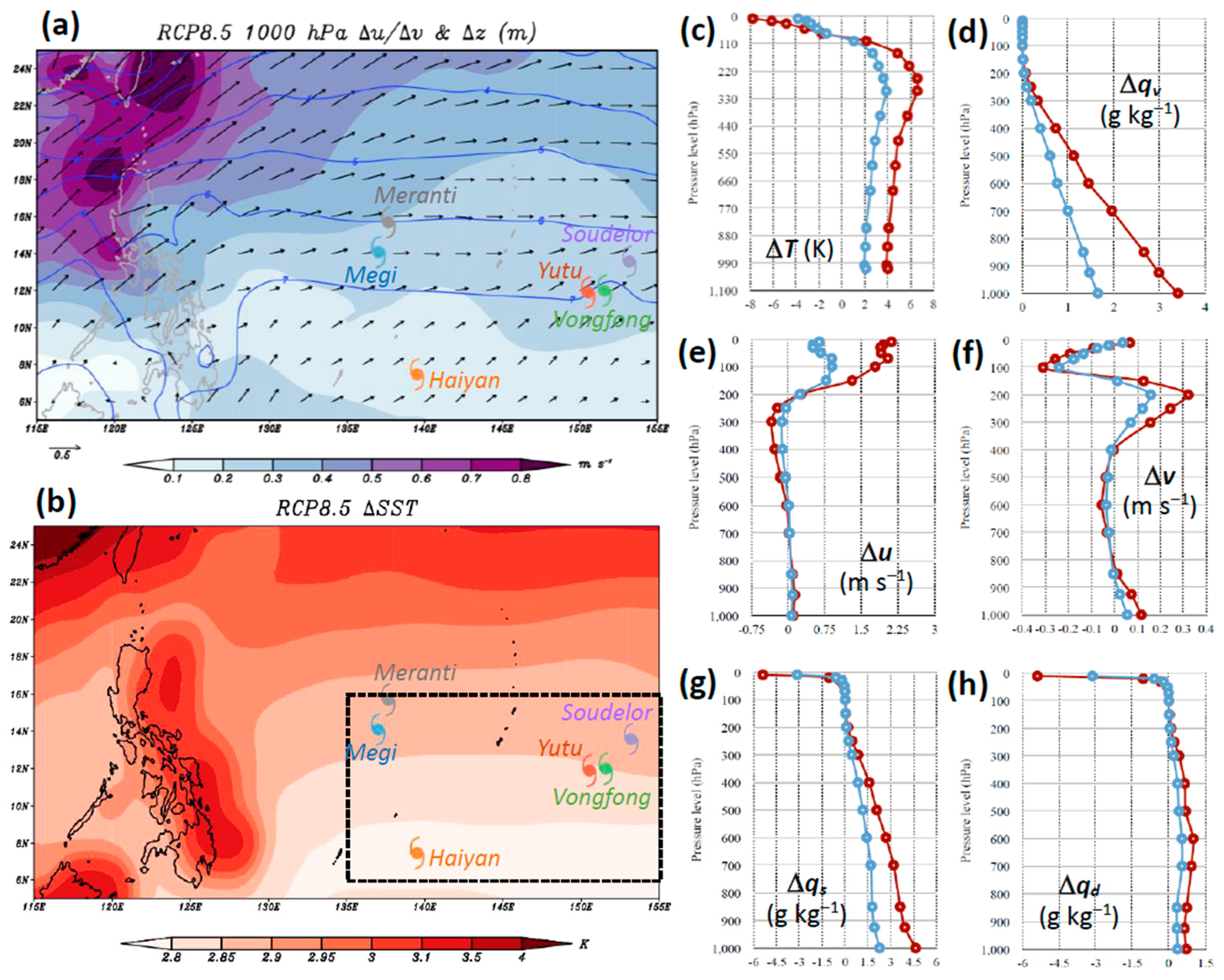
2.2. Estimation of Long-Term Climate Change

Outputs from a total of 38 climate models in the Coupled Model Intercomparison Project Phase 5 (CMIP5) [43,44] are used to compute the projected long-term trend of climate change over 100 years under two projected future emission scenarios, namely, RCP4.5 and RCP8.5, as their mean values. These two scenarios correspond to moderate and high GHG emissions, respectively. Given in

Table 1. List of the CMIP5 models used to compute the long-term trend of projected climate change for June–October from 1981–2000 to 2081–2100. Information includes model number, name, and developer ^#. * An asterisk in the model name indicates that the RCP4.5 results are not available.

No.	Model	Developer	No.	Model	Developer
1	ACCESS1.0	CSIRO-BOM,	21	GISS-E2-R	NASA-GISS, USA
2	ACCESS1.3	Australia	22	GISS-E2-R-CC
3	BCC-CSM1.1	BCC, CMA, China	23	HadGEM2-AO	NIMR-KMA, Korea
4	BCC-CSM1.1(m)		24	HadGEM2-ES	MO-HC, UK
5	CanESM2	CCCma, Canada	25	HadGEM2-CC
6	CCSM4	NCAR, USA	26	INM-CM4	INM, Russia
7	CESM1-BGC	NSF/DOE/NCAR,	27	IPSL-CM5A-LR	IPSL, France
8	CESM1-CAM5	USA	28	IPSL-CM5A-MR
9	CMCC-CM	CMCC, Italy	29	IPSL-CM5B-LR
10	CMCC-CMS		30	MIROC5	AORI/NIES/
11	CNRM-CM5	CNRM, France			JAMSTEC, Japan
12	CSIRO-Mk3-6-0	CSIRO, Australia	31	MIROC-ESM-CHEM *	JAMSTEC, Japan
13	FGOALS-g2	IAP-CAS, China	32	MIROC-ESM
14	FGOALS-s2		33	MPI-ESM-LR	MPI, Germany
15	FIO-ESM *	FIO, SOA, China	34	MPI-ESM-MR
16	GFDL-CM3	GFDL.NOAA, USA	35	MRI-ESM1	JMA-MRI, Japan
17	GFDL-ESM2G		36	MRI-CGCM3
18	GFDL-ESM2M		37	NorESM1-M *	NCC, Norway
19	GISS-E2-H	NASA-GISS, USA	38	NorESM1-ME
20	GISS-E-H-CC

^# For acronyms of models/developers, please refer to https://esgf-node.llnl.gov/projects/cmip5/ (accessed on 3 July 2018).

, the increment in the averages of these 38 CMIP5 models from 1981–2000 to 2081–2100 is calculated as the projected trend of climate change into the future at the centennial timescale (i.e., the Δ value). Only months from June to October are considered to reflect the conditions during the warm season. It is also noted that while all 38 models provide the RCP8.5 results, the RCP4.5 ones are available only in 35 of them. However, due to the large number of models involved, such differences in long-term mean values are considered small and negligible.

The ∆ values include all variables needed in the IC/BCs to drive the CReSS experiments but, of course, are only added into sensitivity tests for future climate scenarios. The results of the long-term trend will be presented and discussed in Section 3.

2.3. Cloud-Resolving Model and Experiments

In this study, all experiments are carried out using the CReSS model of Nagoya University [28,29] at Δx = 2.5 km. In the vertical, there are a total of 60 terrain-following levels, with a model top at 30 km. All clouds in CReSS are treated explicitly, and the double-moment bulk cold-rain scheme with six species [29,45,46,47,48,49] is used to allow for proper treatment in cloud microphysics, including latent heating/cooling (

Table 2. The basic setup and physical options in the CReSS model (v.3.4.3) used in this study.

Grid spacing (x, y, z) *	2.5 km × 2.5 km × 124–655 m (500 m)
Grid dimension	1440 × 1440 × 60 (for Meranti)
Domain size (km)	3660 × 3660 × 30 (for Meranti)
IC/BCs of atmosphere	NCEP FNL analyses (every 0.25° or 0.5°, 26 levels)
Sea surface temperature	HYCOM + NCODA (every 0.08°)
Cloud microphysics	Double-moment bulk cold-rain scheme (six species)
PBL turbulence	1.5-order closure with turbulent kinetic energy prediction
Surface processes	Momentum/energy fluxes and shortwave/longwave radiation
Upper ocean	1D slab model from 0 to 150 m in depth (60 levels)

* The vertical grid spacing (Δz) of CReSS is stretched and smallest at the bottom, and the averaged value is given in the parenthesis.

). Other physical options are mostly the same as in Wang et al. [34,35,36], including parameterizations of turbulence in the planetary boundary layer (PBL) [50,51] and energy/momentum and shortwave and longwave radiation at the surface [52,53], with a substrate model over land [29]. For the upper ocean, a one-dimensional (1D) slab model down to 150 m with 60 levels is used (Table 2).

The National Centers for Environmental Prediction (NCEP, Boulder, USA) Global Forecast System (GFS) final (FNL) analyses are used as the IC/BCs of all simulations [54,55]. This gridded dataset has a horizontal resolution of either 0.5° × 0.5° (before July 2015) or 0.25° × 0.25° (since July 2015) on 26 levels every 6 h (Table 1). Compared to similar analysis and re-analysis products from other major centers, tropical cyclones in the NCEP FNL are often more intense, which is a crucial aspect in the simulation of super-typhoons. For the sea surface temperature (SST), the Hybrid Coordinate Ocean Model (HYCOM) with Navy Coupled Ocean Data Assimilation (NCODA) is used [56]. This dataset is 0.08° × 0.08° in resolution and available at 3-h intervals.

Because of the different tracks of the six typhoons, different model domains and grid dimensions in the horizontal are used, as given in

Table 3. The horizontal grid dimension and simulation period of the six super-typhoon cases.

Typhoon	Grid Dimension (x, y)	Initial Time and Simulation Length
Megi (2010)	1440 × 1296	0000 UTC 15 October 2010, 96 h
Haiyan (2013)	1680 × 864	0000 UTC 6 November 2013, 72 h
Vongfong (2014)	1440 × 1440	1800 UTC 4 October 2014, 120 h
Soudelor (2015)	1824 × 1072	0000 UTC 1 August 2015, 96 h
Meranti (2016)	1440 × 1440	1200 UTC 10 September 2016, 96 h
Yutu (2018)	1728 × 928	0600 UTC, 23 October 2018, 72 h

, with a simulation length of either 3, 4, or 5 days. The model output frequency is set to every 3 h. For each typhoon, the CTL that used only the NCEP FNL analysis as IC/BCs and HYCOM + NDODA as the SST (as in Table 2), i.e., it is a recreation of the TC event as it occurred in modern-day climate, was first determined. This involved considerable testing on different initial times (t₀) until the best result in intensity was obtained, as shown in

Table 4. Comparison of intensity between the JTWC best track and model results (CTL, R4.5, and R8.5) for the six super-typhoon cases, including the minimum center sea-level pressure (p_min, hPa) and maximum wind speed (V_max, m s⁻¹) during their lifetime.

Typhoon	Minimum Pressure (hPa)				Maximum Wind Speed (m s−1)
	JTWC	CTL	R4.5	R8.5	JTWC	CTL	R4.5	R8.5
Megi (2010)	903.0	911.6	912.1	910.7	82.31	69.27	68.08	71.39
Haiyan (2013)	895.0	883.4	894.0	910.2	87.46	77.23	75.15	70.12
Vongfong (2014)	907.0	915.4	917.4	919.2	79.74	58.93	58.21	58.39
Soudelor (2015)	907.0	907.8	910.3	919.6	79.74	60.53	58.50	60.73
Meranti (2016)	895.0	900.1	903.4	905.7	87.46	74.87	69.43	67.64
Yutu (2018)	904.0	917.7	920.5	922.2	77.17	62.83	64.49	60.55

. Compared to the JTWC best-track estimates, the difference in p_min in the CTL runs is 13.7 hPa for Yutu (2018), and those for all other cases are, at most, 8.6 hPa. Likewise, the differences in maximum surface (10 m) wind speed are within 10–20 m s⁻¹ (Table 4). Such results are quite satisfactory for TC intensity, especially for p_min.

Once the CTL is in place, two sensitivity tests are performed for each typhoon using identical model setup in future-climate scenarios, one with the long-term trend (i.e., Δ values) of RCP4.5 scenario and the other with that of RCP8.5 scenario added to the IC/BCs of each time. Thus, we essentially place the historical TC events into a future climate background to test how they might change in rainfall and intensity. Below, these two sensitivity tests corresponding to different GHG-forcing scenarios will be termed simply as R4.5 and R8.5, respectively, and the results will be discussed in Section 5. In the CReSS model for simulations within 120 h, the CO₂ level is not considered.

2.4. Water Budget Analysis

As will be shown later, in R4.5 and R8.5 runs with pseudo-global warming, the typhoons tend to produce more rainfall. To explore deeper into the source of this increase and to better understand the processes involved, a water budget analysis is performed for three typhoons, as in some similar studies [34,35,36]. This analysis makes use of the equation of Trenberth and Guillemot [57], which represents the conservation of total water mass and can be written as

$${\displaystyle \frac{\partial }{\partial t}}\left(w_v+w_h\right)+P=-{{\displaystyle \int }}_0^{\infty }{\rho }_v\left(\nabla ·V\right)dz-{{\displaystyle \int }}_0^{\infty }\left(V·\nabla {\rho }_v\right)dz-{{\displaystyle \int }}_0^{\infty }\nabla ·\left({\rho }_{h}V\right)dz+E+R$$

(1)

where w_v and w_h are the vapor and hydrometeor content in the air column, P is precipitation, ρ_v and ρ_h are the vapor and hydrometeor density, V is the horizontal wind vector, E is evaporation, and R is the residual. The total water content, i.e., w_v + w_h, in the tendency term (TDC) on the left-hand side is defined as

$$w_v+w_h={{\displaystyle \int }}_0^{\infty }\left({\rho }_v+{\rho }_h\right)dz$$

(2)

On the right-hand side of Equation (1), the first three terms are vertical integrals of the convergence (CONV) and advection (ADV) of water vapor and the convergence of hydrometeor flux (CHF), respectively. By definition, the sum of CONV and ADV equals the convergence of vapor flux (CVF), but as a dominant term, it is broken down into two components in Equation (1) to facilitate discussion. In essence, Equation (1) states that the vertically integrated total convergence of water (vapor + hydrometeors) in an air column is used to either make precipitation or remain in the column to moisten the air, with R accounting for all sub-grid scale effects and computational errors. In addition, to a first degree, the difference in CONV between two experiments (such as CTL and R8.5) can be attributed to the difference in the total amount of precipitable water (PW) and/or the integrated horizontal convergence (IHC) in the lower to middle troposphere, so these two parameters are also computed from the surface (sea level) to 5.5 km in height as

$${\mathrm{PW}}_{5.5}={{\displaystyle \int }}_0^{5.5 \mathrm{km}}{\rho }_{v }dz, \mathrm{and}$$

(3)

$${\mathrm{IHC}}_{5.5}=-{{\displaystyle \int }}_0^{5.5 \mathrm{km}}\left(\nabla ·V\right)dz$$

(4)

The water budget calculation is performed over selected periods for a cylindrical volume, and thus, it is in a moving quasi-Lagrangian frame with its origin placed at the typhoon center. Therefore, V in Equations (1) and (4) is the wind vector relative to the TC. The results of the water budget analysis will be presented in Section 5.3.

3. Projected Long-Term Trend of Climate Change

Following the method described in Section 2.2, the long-term trend of climate background for the two RCP scenarios is obtained and shown in Figure 1 for selected variables to assess the likely changes in climate in the future. At 1000 hPa near the surface (Figure 1a), the projected change in winds over the WNP is an increase in southwesterly flow by about 0.2–0.8 m s⁻¹ in RCP8.5, in response to the larger increase in z to the south (by >7 gpm) than to the north (by <4 gpm). The winds change the most near the western periphery of the Pacific, in agreement with several studies on current and likely future changes in East Asian summer monsoons [58,59,60,61]. This, however, also corresponds to a weak anticyclonic shear in the region of the TCs. In Figure 1b, the SST also increases more to the north and near the Philippines (≥3 K) and amounts to a stronger warming over land than the ocean, as expected. The hydrostatic response of this warming pattern is in agreement with the changes in height and wind fields at low levels.

Averaged over the TC area at model initial times in CTL, the vertical profile of Δ for temperature (ΔT) shows warming of about 4 K at low levels that increases to 6.5 K in the upper troposphere for RCP8.5 (Figure 1c), whereas the specific humidity (q_v) increased by 3.4 g kg⁻¹ near the surface that reduces upward almost linearly with respect to pressure (p) until negligible levels near and above 200 hPa (Figure 1d). This amounts to roughly a 20% increase in moisture content. In agreement with Figure 1a, changes in wind components (Δu and Δv) are both positive (southwesterly flow) at low levels below about 750 hPa but become positive in the middle and/or upper levels, in agreement with stronger warming in the upper troposphere in the tropics (Figure 1e,f). While the water vapor content increases, the saturation amount (q_s) in RCP8.5 also increases, and by a greater margin due to the warming, about 4.5 g kg⁻¹ near the surface and decreasing upward (Figure 1g). Thus, although both q_v and relative humidity increase, the saturation deficit (q_d) also becomes larger, by about 0.7–1.1 g kg⁻¹ in the lower to middle troposphere (Figure 1h). In RCP4.5, the vertical profiles for all variables above are similar to those in RCP8.5 throughout the troposphere, except with only about half the magnitude (Figure 1c–h). The same applies to their spatial patterns, so Figure 1a,b only show those in RCP8.5. In summary, the higher water vapor content and SST in future climate are favorable for TC development, and the stronger southwesterly flow at low levels may also increase the moisture supply. However, not all changes are favorable for high intensity and more rainfall, as several other factors might have negative effects. These include the anticyclonic shearing vorticity at low levels (Figure 1a), a reduction in temperature lapse rate in the vertical with higher stability (Figure 1c), the increase in saturation deficit (Figure 1h), and a reduction in the temperature difference across the air/sea interface, since the increase in SST (<3 K) in Figure 1b is less than ΔT (~4 K) at the lowest level (Figure 1c). The increase in z at 1000 hPa (Figure 1a) also implies that the TC’s minimum central pressure p_min would be higher at t₀ of future-scenario runs by about 0.5 hPa for RCP8.5.

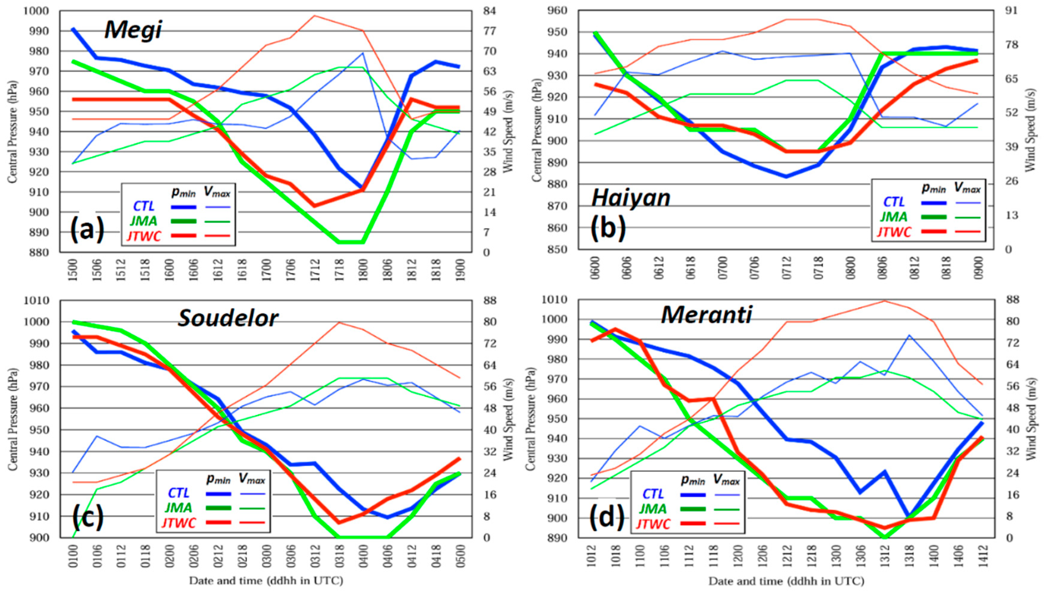
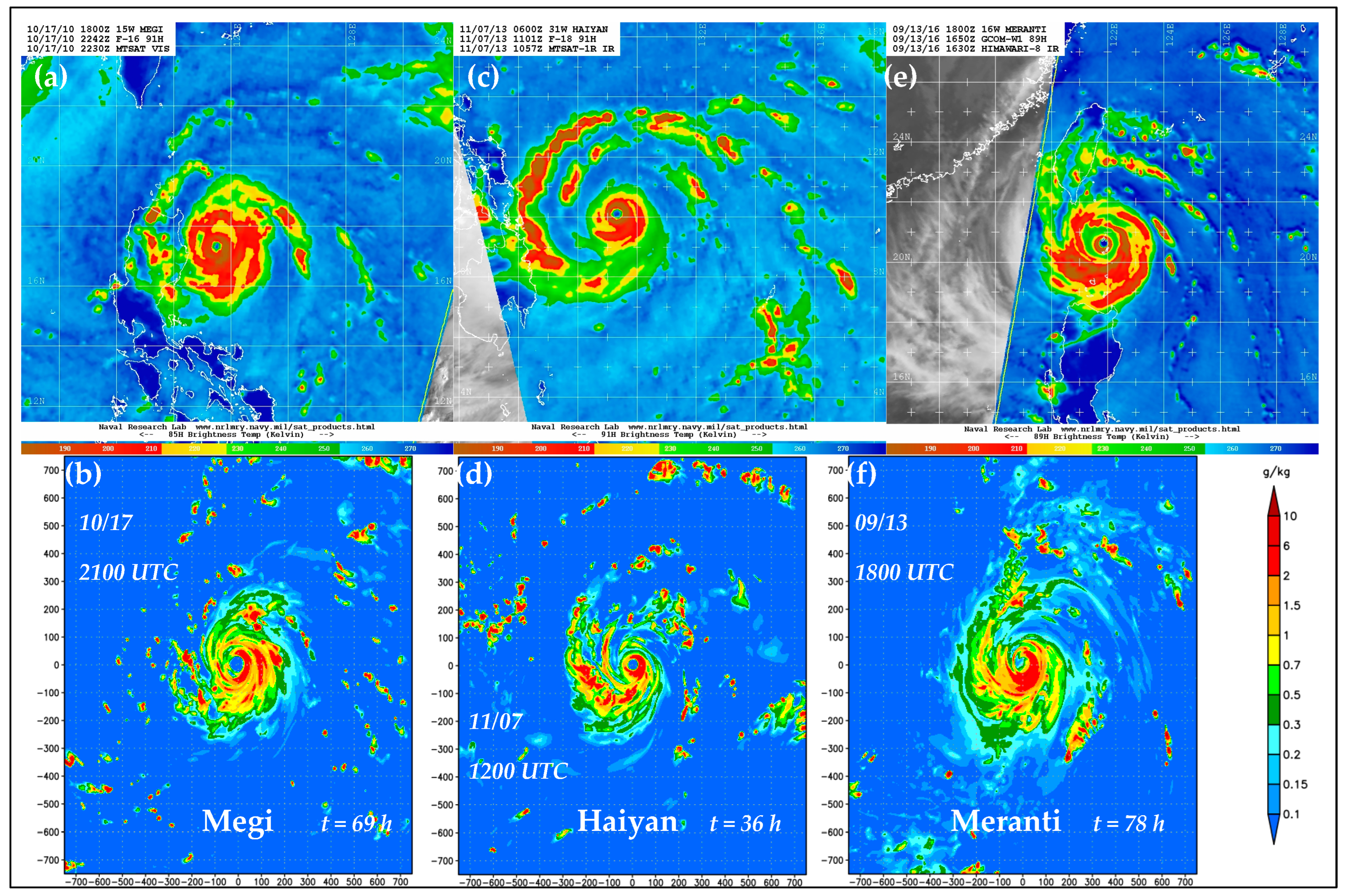
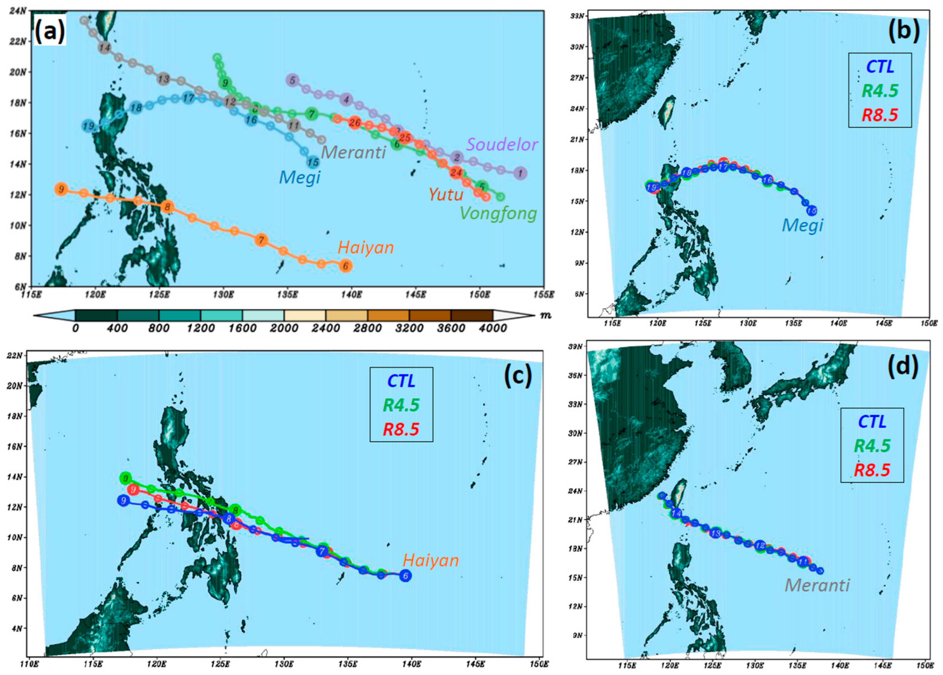
4. Overall Results of Control Experiments

In this section, the CTL results of the typhoons are validated against the observations. Figure 2 shows the comparison between the best tracks and model-simulated tracks in CTL for all six typhoons (note that the length scale is not the same among panels). Among them, the track errors around 0000 UTC 16 October for STY Megi (2010) are the largest, but still about 100 km and not too large (Figure 2a). For all other typhoons, the track errors rarely exceed about 60 km (Figure 2b–f). Thus, the overall performance in CTL runs in TC tracks is quite satisfactory.

While the information on peak intensity (p_min and V_max) attained in the CTL runs is included and compared with the JTWC best track in Table 4, the time evolution is shown in Figure 3 for 4 of the super-typhoons. Between the two best tracks, JMA tends to estimate a lower p_min than the JTWC at times, but considerably lower V_max as it uses 10-min averages, whereas the JTWC uses 1-min averages. Near peak intensity, their difference in V_max is about 15–20 m s⁻¹ or so and not small. As already discussed in Section 2.3, the CTL runs give satisfactory results in p_min, typically within 10 hPa to JTWC. For V_max, the model values tend to be closer to the JMA (e.g., Figure 3a,c) or between the two best tracks (e.g., Figure 3b,d). Note that the CTL for Haiyan is the only one that yielded a considerably lower p_min than the estimates (by 11.6 hPa). Not shown in Figure 3, the CTL result for Vongfong is similar to that for Soudelor, and that for Yutu is similar to Meranti. As mentioned, in terms of intensity, these CTLs are already the best results achievable with substantial testing.

In Figure 4, three pairs of observed and modeled convection and cloud structures are presented and compared, one pair for each of Megi, Haiyan, and Meranti at a selected time during or near their peak intensity with data available. In all three instances, one can see that the CReSS, with a Δx of 2.5 km, can simulate the cloud structure of these intense TCs quite realistically, even though the TRMM brightness temperature (T_B) and column-maximum mixing ratio of precipitating particles (rain, snow, plus graupel) are not identical quantities. The simulated rainfall accumulation at different stages also exhibits good agreement with the GPM IMERG data. Many past studies have also demonstrated and confirmed such a capability, e.g., [62,63,64]. In the case of Meranti, a minor deficiency also exists in that the small inner eyewall in the satellite image (Figure 4e) is not well captured in CTL (Figure 4f). Nevertheless, overall, the results of the CTL runs are realistic and satisfactory, and they will next serve as benchmarks for comparison when the same TCs are placed in future climate in the RCP4.5 and RCP 8.5 scenarios.

5. Potential Impacts of Future Climate Change on Intense Typhoons

5.1. Track and Intensity

From Figure 5, it is seen that the tracks of the three TCs shown in R4.5 and R8.5 tests are all very similar to those in CTL when the respective Δ values are added into the IC/BCs (while all other settings are identical). The largest differences in TC center positions occur near the end of the simulation for Haiyan, close to 100 km (Figure 5c), and the differences are also larger at roughly 55 km around 0000 UTC 17 October for Megi (Figure 5b). For Meranti, the differences are all within half of a degree (Figure 5d). For Soudelor, Vongfong, and Yutu, the track errors are comparable or smaller, and thus, their figures are not shown. Thus, adding Δ values into the IC/BCs has only small effects on the tracks of these intense TCs, in agreement with some earlier studies, e.g., [34,35,36,37].

In terms of intensity, the time series of p_min and V_max of all six typhoons in the three experiments of CTL, R4.5, and R8.5 are compared in Figure 6, and Table 4 also contains the highest values achieved at peak intensity. Between these two scenarios, RCP8.5 corresponds to larger changes in the long-term climate (Figure 1), and thus, we focus more on the R8.5 results here due to their greater responses. Among all cases, Megi is the only one for which the future scenario in RCP8.5 yields a more intense TC compared to the present-day climate, but only barely (Figure 6a). In R8.5, the p_min is 0.9 hPa deeper, and V_max is 2.1 m s⁻¹ stronger (also Table 4). The R4.5 run for Megi produces an intensity slightly weaker than the CTL during most of the simulation period, but the differences are rather small.

For all other five super-typhoons, their intensity tends to be weaker in future scenarios, especially the RCP8.5, than their present-day counterpart (Figure 6b–f). This is often true in both p_min and V_max but could be more obvious in one parameter than the other. For Vongfong, Meranti, and Yutu (Figure 6c,e,f), the differences in intensity are quite small, and the p_min is about 2–3 hPa higher in R4.5 (than the one in CTL), and another 2–3 hPa higher in R8.5. For Soudelor, the weakening in p_min in R8.5 is larger by comparison, at 11.8 hPa, but no reduction in V_max (Figure 6c, Table 4). The most obvious weakening occurs in Haiyan (Figure 6b), in which the p_min rises by 10.6 hPa and V_max reduces by 2.08 m s⁻¹ in R4.5 compared to CTL, and further by another 16.2 hPa and 5.03 m s⁻¹ from R4.5 to R8.5, respectively. In other words, the future scenarios for Haiyan are much weaker, particularly for the RCP8.5 scenario, and these deficits are apparent in Figure 6b prior to the TC’s landfall in the Philippines on 8 November. While slightly higher p_min values at t₀ in the experiments for future scenarios to begin with, as mentioned in Section 3, are also depicted and noticeable in Figure 6, for all cases except Megi, a weaker TC peak intensity in a warmer and moister climate background is nevertheless counter-intuitive and not expected. Possible reasons for such a result, especially for Haiyan, will be further explored and discussed in Section 6.

5.2. Precipitation

To assess changes in precipitation, the averaged rainfall (per 3 h) inside the radii of 200, 250, 300, 350, and 400 km from the TC center over the full simulation period in CTL, R4.5, and R8.5 for the six typhoons are presented in

Table 5. Areal-averaged rainfall (mm per 3 h) inside the radii of 200, 300, and 400 km from the TC center over the full simulation period in CTL, R4.5, and R8.5 for the six typhoons, and the percent change (%) in the two future RCP scenarios relative to CTL.

Typhoon	Exp.	200 km		250 km		300 km		350 km		400 km
		Rain	Ch.	Rain	Ch.	Rain	Ch.	Rain	Ch.	Rain	Ch.
Megi (2010)	CTL R4.5 R8.5	20.58 22.85 24.70	− +11.00 +19.99	16.47 17.84 19.37	− +8.33 +17.58	13.22 14.07 15.29	− +6.43 +15.64	10.66 11.32 12.14	− +6.17 +13.90	8.70 9.23 9.82	− +6.04 +12.85
Haiyan (2013)	CTL R4.5 R8.5	26.19 28.91 31.27	− +10.42 +19.43	20.49 22.00 24.82	− +7.4 +21.16	16.21 17.40 19.93	− +7.36 +23.00	13.18 14.43 16.59	− +9.51 +21.84	11.04 12.46 14.31	− +12.85 +29.60
Vongfong (2014)	CTL R4.5 R8.5	21.19 22.81 26.21	− +7.62 +23.70	16.66 18.00 18.80	− +8.10 +12.86	13.86 14.62 14.08	− +5.52 +1.61	11.55 11.76 10.81	− +1.87 −6.40	9.50 9.44 8.51	− −0.71 −10.40
Soudelor (2015)	CTL R4.5 R8.5	15.59 17.46 19.32	− +11.98 +23.90	12.80 14.04 15.27	− +9.63 +19.28	10.85 11.56 12.08	− +6.58 +11.29	9.16 9.48 9.73	− +3.43 +6.24	7.74 7.97 8.14	− +3.00 +5.15
Meranti (2016)	CTL R4.5 R8.5	20.14 21.33 24.09	− +5.92 +19.58	15.81 16.72 18.60	− +5.75 +17.65	13.03 13.50 15.07	− +3.64 +15.66	10.56 11.05 11.79	− +4.67 +11.67	8.73 9.13 9.28	− +4.63 +6.30
Yutu (2018)	CTL R4.5 R8.5	24.11 25.81 26.85	− +7.06 +11.37	19.18 19.97 20.90	− +4.13 +8.98	15.44 15.81 15.86	− +2.41 +2.76	12.06 12.22 11.92	− +1.35 −1.15	9.49 9.54 9.31	− +0.61 −1.82

, together with the percent changes in the two future scenarios from the CTL. For all TC cases, their rainfall increases in a warmer and wetter future climate, so results in rainfall are much more consistent in our study. In R4.5, the total rainfall increases by about 2.5–7% inside 300 km, 4–10% inside 250 km, and 6–12% inside 200 km, respectively. These figures are roughly doubled in R8.5 for most cases, and the increases are by about 2–23% inside 300 km, 9–21% inside 250 km, and 11.5–24% inside 200 km, respectively. At smaller radii near the inner core (e.g., 200 km), the increases are more consistent and less variable among the cases, by close to 10% in R4.5 and 20% in R8.5 in most cases. Further away from the TC center, a higher variability is seen among the cases, but the R8.5 runs also tend to produce more rain than the R4.5, except for Vongfong and Yutu. Overall, such increases are comparable to many earlier studies, e.g., [1,2,11,12,13,14], and the increase in the amount of moisture in the two scenarios. Note that the general agreement in rainfall changes also extends to studies for other basins, presumably because the projected long-term trend due to global warming is similar.

In Figure 7, radial profiles of azimuthally-averaged 3 h rainfall and the time series of areal-mean rainfall inside a selected radius over the simulation period for three TCs, Megi, Haiyan, and Meranti, are shown as examples. The chosen radius is 350 km for Megi, 250 km for Haiyan, and 300 km for Meranti, and the same are used later for water budget analysis. From the radial profiles, it is clear that all three TCs produce more rainfall in future scenarios inside about 200 km (Figure 7a,c,e), and similar differences also extend outward to almost 500 km for Haiyan. In the time series of mean rainfall inside the selected radius from the TC center, it is also seen that the increased rainfall in future climate scenarios is rather persistent throughout the full simulation length, except for occasional short periods of time (Figure 7b,d,f). For Megi and Meranti, the future runs also have less rainfall than the CTL in the first 6–9 h after t₀, most likely due to the increased deficit before saturation, as seen in Figure 1h. Overall, the more abundant TC rainfall in future climate is a robust feature among all six cases (Table 5). On the other hand, Haiyan’s peak rainfall in the eyewall occurs at a larger radius in both R4.5 and R8.5, indicative and consistent with the weaker simulated intensity in future scenarios.

Associated with warming (see Figure 1c), some changes in the mean structure of the TCs are also seen in R4.5 and R8.5 and are perhaps worthy of discussion. In Figure 8, the example of Haiyan is shown out to a radius of 400 km. In CTL, Haiyan develops to a height of roughly 17 km, with strong inflow below 2 km, upward motion between 30 and 60 km (inside the eyewall) from the center, and strong outflow over 13–17 km in height (Figure 8a). With the 0 °C isotherm (melting level) located near 5.2 km, graupel is mostly above 4 km, and raindrops are mostly below 5.5 km (Figure 8b,c). In R8.5, the storm can develop higher to almost 19 km, with eyewall updrafts also extending higher and producing outflow at 16–19 km (Figure 8d). On average, the rising motion strengthens along the outer edge of the eyewall but, however, weakens along the inner edge in R8.5, again signaling a larger eye and weaker intensity. Because the 0 °C isotherm is raised to at least 6 km in R8.5 (by ≥800 m), graupel now appears higher, and its amount reduces near 4.5–6 km (Figure 8e), where raindrops increase in amount instead (Figure 8f). Likewise, ice particles in R8.5 can appear higher as well, up to more than 20 km above the eyewall updrafts. Rather consistent among all six TCs, these changes in response to the warming are expected and quite interesting.

Owing to the fact that the statistical tests are performed for “paired” samples for the same events, as opposed to two groups of different, independent events in two different climate backgrounds, high confidence can be established from the results of PGW experiments with relative ease, as discussed in Section 1 and shown previously [34,35,36]. Thus, we also briefly present the test results for Megi, Haiyan, and Meranti here. For paired samples, the one-tail t-test is used, e.g., [65], on mean 3 h rainfall inside fixed radii from the TC center (as shown in the right column in Figure 7 for one radius). The null hypothesis here is that the rainfall does not increase in the future run from the CTL, and it is rejected, i.e., the increase is statistically significant if the computed t value exceeds the criterion at the selected confidence level. The results of this test are shown in

Table 6. The t-test results (t values) for 3 h rainfall changes (mm per 3 h) in the two future scenarios (R4.5—CTL and R8.5—CTL) inside the radii of 200, 250, 300, 350, and 400 km from the TC center over the full simulation period for Megi (n = 32), Haiyan (n = 24), and Meranti (n = 32, top half), and the criteria for t value at five confidence levels from 90.0% to 99.9% (bottom half).

Typhoon	n	Experiment	200 km	250 km	300 km	350 km	400 km
Megi (2010)	32	R4.5—CTL R8.5—CTL	5.183 7.700	6.249 8.432	5.100 8.646	4.306 7.443	4.805 6.761
Haiyan (2013)	24	R4.5—CTL R8.5—CTL	4.298 5.158	3.084 6.146	3.240 7.067	4.586 8.169	5.746 9.810
Meranti (2016)	32	R4.5—CTL R8.5—CTL	3.951 5.799	3.859 5.450	2.207 5.290	2.842 3.945	2.585 2.359
Confidence level			90.0%	95.0%	99.0%	99.5%	99.9%
n = 24			1.320	1.714	2.500	2.807	3.485
n = 32			1.309	1.696	2.453	2.744	3.375

. One can see that for rainfall increases in R8.5, the t values are all at least about 4 and were significant at the highest confidence level of 99.9%, with the lone exception at 400 km for Meranti (significant at 95%). For R4.5, where the amounts of increase are less (see Table 5), again, the increments are significant at a level of ≥99.5% for all five radii for the three cases, except for Meranti at 300 km (95%). Regardless, the increase in TC rainfall in the future climate is robust and tested to be highly significant statistically.

5.3. Water Budget Analysis

As described in Section 2.4, the water budget is calculated for a cylindrical column inside a selected radius r for Megi at r = 350 km, Haiyan at r = 250 km, and for Meranti at r = 300 km. Using plots like those in Figure 4 (bottom row), these radii are selected to include most of the TC rainfall. The calculation, however, is not for the full simulation period, but for t = 6–90 h (excluding the first and last 6 h) for both Megi and Meranti and for t = 24–72 h (excluding the first day) for Haiyan, so as to keep the residual (R) at a relatively low level. The water budget results are presented in

Table 7. Results of water budget analysis for Megi, Haiyan, and Meranti for a cylindrical column inside a selected radius over a chosen period in CTL, R4.5, and R8.5, and their differences (future minus present). The different terms are precipitation (P), tendency of total water contents (TDC), convergence of vapor flux (CVF), convergence of hydrometeor flux (CHF), evaporation (E), and residual (R). CVF is further partitioned into convergence (CONV) and advection (ADV) of vapor by horizontal winds. All units are in mm per 3 h (or kg m⁻² per 3 h).

Typhoon	Experiment	P	TDC	CVF	CONV	ADV	CHF	E	R
Megi (2010) (r = 350 km) (t = 6–90 h)	CTL R4.5 R8.5	10.79 11.48 12.47	0.21 0.25 0.29	9.48 10.37 11.31	10.58 11.45 12.50	−1.10 −1.07 −1.19	−0.08 −0.06 −0.06	1.41 1.46 1.54	+0.19 −0.04 −0.02
	R4.5—CTL R8.5—CTL	+0.69 +1.68	+0.04 +0.08	+0.89 +1.83	+0.87 +1.93	+0.03 −0.09	+0.02 +0.02	+0.05 +0.13	− −
Haiyan (2013) (r = 250 km) (t = 24–72 h)	CTL R4.5 R8.5	19.16 21.48 23.75	0.15 0.19 0.29	15.85 17.05 19.24	17.19 18.44 20.82	−1.34 −1.38 −1.58	+0.10 +0.07 +0.21	1.80 1.84 2.03	+1.57 +2.70 +2.57
	R4.5—CTL R8.5—CTL	+2.32 +4.59	+0.04 +0.14	+1.20 +3.39	+1.25 +3.63	−0.04 −0.24	−0.03 +0.11	+0.04 +0.23	− −
Meranti (2016) (r = 300 km) (t = 6–90 h)	CTL R4.5 R8.5	13.36 14.03 15.49	0.13 0.15 0.24	11.15 12.54 15.75	12.35 13.82 17.32	−1.21 −1.28 −1.58	+0.12 +0.11 −0.03	1.52 1.59 1.56	+0.70 −0.06 −1.55
	R4.5—CTL R8.5—CTL	+0.67 +2.13	+0.02 +0.11	+1.39 +4.60	+1.46 +4.97	−0.07 −0.37	−0.01 −0.15	+0.07 +0.03	− −

.

In Table 7, it is seen that the TC total precipitation P (10.8–23.8 mm, per 3 h) comes mainly from the CVF into the cylinder from the lateral side (9.5–19.2 mm), with a secondary source of water in evaporation E from the ocean beneath (1.4–2.0 mm). With absolute values within 0.2–0.3 mm (per 3 h), the TDC and CHF terms are both small and almost negligible, while R is also small in some runs and kept within about 12.5% of P (R4.5 of Haiyan), as the same period must be used in the same TC for all three runs of CTL, R4.5, and R8.5. The CVF is mainly contributed by the CONV term (10.6–20.8 mm), which tends to be larger than the CVF to offset the negative vapor advection effect by the low-level inflow from drier surroundings in ADV (roughly between −1.1 and −1.6 mm). For the increases in rainfall in R4.5 and R8.5 (0.7–4.6 mm per 3 h), they are also largely accounted for by increases in CONV (0.9–5.0 mm) in the CVF term (0.9–4.6 mm).

In

Table 8. Similar to Table 7, but showing the results of CONV (mm per 3 h, as in Table 7) and the two related parameters of precipitable water below 5.5 km (PW_5.5, mm) and integrated horizontal convergence below 5.5 km (IHC_5.5, 10⁻² m s⁻¹) in CTL and their changes in R4.5 and R8.5 (future minus present), respectively, in the three typhoons. The changes are also given in percent (%).

Typhoon	Experiment	CONV		PW5.5		IHC5.5
Megi (2010)	CTL	10.58		53.11		5.45
(r = 350 km) (t = 6–90 h)	R4.5—CTL R8.5—CTL	+0.87 +1.93	+8.2% +18.2%	+6.78 +12.66	+12.8% +23.8%	−0.17 −0.08	−3.0% −1.5%
Haiyan (2013)	CTL	17.19		53.11		10.29
(r = 250 km) (t = 24–72 h)	R4.5—CTL R8.5—CTL	+1.25 +3.63	+7.3% +21.1%	+7.04 +13.26	+13.3% +25.0%	−0.51 +0.08	−5.0% +0.7%
Meranti (2016)	CTL	12.35		54.39		7.64
(r = 300 km) (t = 6–90 h)	R4.5—CTL R8.5—CTL	+1.46 +4.97	+11.9% +40.2%	+7.12 +14.15	+13.0% +25.8%	−0.01 +0.64	−0.2% +8.4%

, the values of CONV (as in Table 7) are further broken down to the two relevant parameters of PW_5.5 and IHC_5.5, as shown in Equations (1), (3), and (4), and how much they change in R4.5 and R8.5 compared to the reference of CTL. While CONV increased by about 7–12% in R4.5 and by about 18–40% in R8.5, the increase in PW_5.5, which is between 53.1 and 54.4 mm in CTL, is almost the same, by 13% in R4.5 and 24–26% in R8.5. Such a nearly constant increase in precipitable water in the TC environment, somewhat higher than the Δ values, is perhaps not surprising. Compared to PW_5.5, the changes in IHC_5.5 are much more variable and are all slightly negative in R4.5 and between −1.5% and +8.5% in R8.5. In many instances in Table 8, the product of change in PW_5.5 and that in IHC_5.5 gives a fairly close approximation to the change in CONV. Overall, it can be concluded that the increase in rainfall in R4.5 and R8.5 is mainly due to increased moisture content (i.e., PW). The negative or less contribution from IHC_5.5 by comparison, is in general agreement with the limited difference in intensity.

6. Discussion

While consistent results are obtained in our PGW experiments for rainfall brought by all six super-typhoons in the WNP, with increases of roughly 10% in R4.5 and 20% in R8.5 inside a radius of 200–250 km from the TC center (Table 5 and Figure 7), mainly due to the more abundant moisture in the background in the two future scenarios (Table 8). For intensity, on the contrary, most TCs weaken slightly, but Haiyan weakens substantially in future climate (Table 4 and Figure 6). While some studies also suggest relatively few changes in TC intensity during the past several decades, e.g., [31,34,36,66], our result of the future projection of some of the most intense storms is still counter-intuitive and not consistent with most projection studies in the literature, e.g., [1,2,5,9,11,12,13,14]. Thus, here we discuss the likely reasons for our result and the limitation of the PGW approach to address issues like the intensity change of such intense TCs.

In Figure 1, some changes shown as Δ values are identified to potentially exert negative effects on subsequent TC intensity, such as a weaker cyclonic vorticity and higher p_min at t₀ (Figure 1a), a reduced temperature lapse rate with higher stability (Figure 1c), a smaller air/sea temperature difference (also Figure 1b), and an increase in saturation deficit (Figure 1h). The effects of a slightly weaker initial vortex and the increase in q_d have been discussed and seem to be small and confined to the first several hours of the experiment. Given the substantial increase in rainfall in future scenarios, the small changes in the lapse rate are also not likely to explain the weaker TC intensity.

In Section 1, the study of Tsuboki et al. [25] was reviewed as an example. In this study, 2 km downscaling experiments were performed on two groups of the 30 most intense TCs in the WNP simulated by a GCM, one in modern-day climate and the other in future climate (a total of 60 TCs). Since, on average, the storms in the future climate were stronger in the GCM to begin with, the 2 km runs further enlarged the differences among the two TC groups using an identical process for downscaling. Thus, it is a valid method to address the potential impact of climate change on TC intensity (but somehow not as easy to establish the statistical significance).

In the PGW method as adopted in this study, however, an advantage in CTL (under the present climate) was artificially and unintentionally introduced during the tests for the best t₀, which gave the strongest intensity, as described in Section 2.3. This means that the t₀ and IC/BCs selected were best suited for CTL to produce the strongest storm. This appears to be particularly true for Haiyan, as its CTL yielded a storm of 883.4 hPa in p_min, 11.6 hPa deeper than the JTWC estimate of 895 hPa (Table 4). Once the Δ values are added for R4.5 or R8.5, the IC/BCs are changed, which may be small within the TC vortex but not necessarily so in the environment farther away. Thus, apart from some negative impact of the Δ values as pointed out above, the interaction between the TC and its environment during the simulation of R4.5 and R8.5 became not as favorable for further rapid intensification, which is a very delicate and complex dynamical process involving latent heat release, e.g., [67,68,69,70]. Such small differences introduced by the Δ values apparently had more impact on Haiyan, so bifurcation in intensity starts to occur after 9 h in the three runs (Figure 6b). Compared to the other five storms, Haiyan also developed and traveled westward at a much lower latitude (see Figure 5a), where the increases in SST in the RCP scenarios are smaller (Figure 1b).

To provide further information regarding the effects of Δ values (i.e., long-term trend) in future scenarios, some additional tests were performed where certain variables were not added into the IC/BCs for the RCP8.5 scenario, particularly for Haiyan, as summarized in

Table 9. Results of additional sensitivity tests on p_min (hPa) by withholding some of the Δ values for the RCP8.5 scenario from adding into the IC/BCs for Haiyan, Megi, and Meranti. The Δ values are separated into three groups: wind field (u/v), thermodynamic field (z/T/SST), and moisture field (q_v). Those added are denoted by a check mark, and “cQd” means constant saturation deficit (q_d). The p_min values from CTL and R8.5 are the same as those in Table 4.

Experiment	Δ Values for RCP8.5			Minimum Pressure (pmin, hPa)
	u/v	z/T/SST	qv	Haiyan	Megi	Meranti
CTL R8.5	√	√	√	883.4 910.2	911.6 910.7	900.1 905.7
R8.5_nW R8.5_nQ R8.5_nWQ	√	√ √ √	√	909.5 911.9 900.3	910.4 928.3 931.6	905.1 907.6 909.2
R8.5_nWT R8.5_cQd	√	√	√ cQd	926.3 905.2	− −	− −

. All Δ variables are classified into three groups: kinematic (wind), thermodynamic, and moisture fields, and the same group is added or removed together as a unit (because it is inconsistent to have one or some without the others). While these additional tests should be compared with R8.5, Δq_v in moisture is more important than the other variables for Megi and Meranti (Table 9). This is especially true for Megi, as it is much weaker without the addition of Δq_v. For Haiyan, on the other hand, both Δu/Δv and Δq_v have a negative effect on intensity, which is apparently being helped the most by ΔSST. Among the new tests, the lowest p_min is 900.3 hPa in R8.5_nWQ when only the thermal fields are added. The second lowest p_min is 905.2 hPa when all Δ variables are added as in R8.5, except that Δq_s rather than Δq_v is added to keep q_d the same as in CTL. So, Haiyan’s intensity is also hampered by the increase in q_d in its environment at lower latitudes in R4.5 and R8.5. Without adding the thermal fields, the p_min rises substantially from 909.5 hPa in R8.5_nW to 926.3 hPa in R8.5_nWT, the weakest among all tests. Among the three thermal variables, the increase in SST is considered the most helpful to Haiyan’s intensity, as tested previously [71,72]. In [72], the authors suggested that the intensity of Haiyan would increase the most if only ΔSST is added, but not as much if the projected trend in T and moisture are also taken into account. Overall, while some aspects of our results are in agreement with earlier studies, it is recommended to practice caution when applying the PGW method similar to this one to assess the impact of global warming on the intensity of strong TCs. Perhaps t₀ in runs for future scenarios can also be tested and does not need to be kept the same, or an ensemble approach can be used, such that the advantage gained in the IC/BCs of the CTL can be remedied to some degree. In fact, for rainfall attribution of TY Morakot (2009), ref. [37] used a large ensemble size with random noises in the IC, and the ensemble mean was quite close to those from sensitivity tests without ensemble [34,35,36]. For intensity, nevertheless, the ensemble method might be worthwhile but is for further study in the future to consider.

7. Conclusions and Summary

In this study, potential impacts of long-term climate changes toward the end of the twenty-first century under RCP4.5 and RCP8.5 scenarios (medium and high emissions, respectively) on intense typhoons in the WNP are assessed using cloud-resolving simulations (with a grid size of 2.5 km) and the PGW approach, mainly in two aspects of the TCs: rainfall and intensity. A total of six super-typhoons in recent years are included: Megi (2010), Haiyan (2013), Vongfong (2014), Soudelor (2015), Meranti (2016), and Yutu (2018), while the long-term linear trends (Δ values) over 100 years in the two scenarios are estimated from 38 CMIP5 models between two 20-year averages for June–October (from 1981–2000 to 2081–2100). For each case, a control experiment (CTL) using the NCEP FNL analysis and HYCOM + NCODA SST as IC/BCs was first determined to best reproduce the event. Then, sensitivity tests, named simply as R4.5 and R8.5, were carried out for future climate scenarios with identical settings, except that the Δ values are added into the IC/BCs throughout the simulation. By comparing the three runs for each TC, the possible changes in the future scenarios can be assessed. The main results are summarized below.

Obtained from 38 CMIP5 models, the projected long-term trend at the centennial scale in the TC formation region of the WNP in RCP8.5 includes increases in SST of ~3 °C and in air temperature of ~4 °C at the lower troposphere, increasing to 6.5 °C near the tropopause, and increases in moisture by roughly 20%. Consistent with greater warming over land than the ocean, the East Asian southwesterly summer monsoon at low levels also strengthens by up to 0.7 m s⁻¹ near the land/sea boundary. Associated with these changes, a few factors may become less favorable for TC development, including a weaker initial vortex, a smaller air/sea temperature difference, and an increase in saturation deficit despite more moisture. All Δ values of RCP4.5 exhibit similar spatial patterns to those of RCP8.5 but at about half the magnitude.

In future scenarios, TC precipitation all increases inside 300 km from the center and is more consistent among the six super-typhoons by about 2–23% inside 300 km, 9–21% inside 250 km, and 11.5–24% inside 200 km, respectively, in R8.5 compared to the CTL. The corresponding figures in R4.5 are roughly halved. Inside 200–250 km, the rainfall increases near the inner core are also less variable and more consistent, by close to 10% in R4.5 and 20% in R8.5 in most cases, and can be largely explained by the more abundant background moisture and subsequent vapor convergence through the water budget analysis. As paired samples, the increase in rainfall is also tested to be highly significant statistically, mostly at the confidence level of 99.9% (all ≥95%). Associated with the warming, the total depth of the TCs also increases from about 17 to 19 km, and the melting level height is raised by around 0.8 km in RCP8.5.

For TC peak intensity in terms of p_min and V_max, however, except for Megi, all five other TCs become weaker in future scenarios. Evolving at lower latitudes, Haiyan’s weakening in p_min is particularly significant. Thus, our result is not consistent with most studies in the literature. It is believed that in determining the initial time (t₀) for CTL, which gave the strongest TC closest to the best track data, sometimes within a few hPa, an advantage is unintentionally introduced to the CTL. Once the Δ values are added in R4.5 and R8.5, small differences are introduced into the environment, which becomes not as favorable for subsequent TC intensification. Thus, the PGW approach adopted here may have some bias in assessing the peak strength of intense TCs. At least, caution needs to be practiced.

References

1. IPCC. Climate Change 2013: The Physical Science Basis. Contribution of Working Group I to the Fifth Assessment Report of the Intergovernmental Panel on Climate Change; Stocker, T.F., Qin, G.-K., Plattner, M., Tignor, S.K., Allen, J., Boschung, A., Nauels, Y., Xia, V., Bex, Midgley, P.M., Eds.; Cambridge University Press: Cambridge, UK; New York, NY, USA, 2013; p. 1535. [Google Scholar]
2. IPCC. Climate Change 2021: The Physical Science Basis. Contribution of Working Group I to the Sixth Assessment Report of the Intergovernmental Panel on Climate Change; Masson-Delmotte, V., Zhai, P., Pirani, A., Connors, S.L., Péan, C., Berger, S., Caud, N., Chen, Y., Goldfarb, L., Gomis, M.I., et al., Eds.; Cambridge University Press: Cambridge, UK; New York, NY, USA, 2021; in press. [Google Scholar] [CrossRef]
3. IPCC. 2018: Global Warming of 1.5 °C. An IPCC Special Report on the Impacts of Global Warming of 1.5 °C above Pre-Industrial Levels and Related Global Greenhouse Gas Emission Pathways, in the Context of Strengthening the Global Response to the Threat of Climate Change, Sustainable Development, and Efforts to Eradicate Poverty; Masson-Delmotte, V., Zhai, P., Pörtner, H.O., Roberts, D., Skea, J., Shukla, P.R., Pirani, A., Moufouma-Okia, W., Péan, C., Pidcock, R., et al., Eds.; in press; Available online: https://www.ipcc.ch/sr15/ (accessed on 25 March 2020).
4. Neumann, C.J. A Global Tropical Cyclone Climatology. Global Guide to Tropical Cyclone Forecasting WMO-No. 1194; World Meteorological Organization (WMO): Geneva, Switzerland, 2017; pp. 28–62. Available online: https://cyclone.wmo.int/ (accessed on 18 August 2020).
5. Li, Y.; Tang, Y.; Li, X.; Song, X.; Wang, Q. 2023: Recent increase in the potential threat of western North Pacific tropical cyclones. Npj Clim. Atmos. Sci. 2023, 6, 53. [Google Scholar] [CrossRef]
6. Normile, D. After the Deluge. Science 2014, 344, 355–357. [Google Scholar] [CrossRef] [PubMed]
7. Shimada, U.; Kubota, H.; Yamada, H.; Cayanan, E.O.; Hilario, F.D. Intensity and inner-core structure of Typhoon Haiyan (2013) near landfall: Doppler radar analysis. Mon. Weather Rev. 2018, 146, 583–597. [Google Scholar] [CrossRef]
8. Normile, D. Deadly typhoon forces Japan to face its vulnerability to increasingly powerful storms. Science 2019. [Google Scholar] [CrossRef]
9. Knutson, T.R.; McBride, C.J.; Emanuel, K.; Holland, G.; Landsea, C.; Held, I.; Kossin, J.P.; Srivastava, A.K.; Sugi, M. Tropical cyclones and climate change. Nat. Geosci. 2010, 3, 157–163. [Google Scholar] [CrossRef]
10. Emanuel, K.A. Increasing destructiveness of tropical cyclones over the past 30 years. Nature 2005, 436, 686–688. [Google Scholar] [CrossRef]
11. Knutson, T.R.; Sirutis, J.J.; Zhao, M.; Tuleya, R.E.; Bender, M.; Vecchi, G.A.; Villarini, G.; Chavas, D. Global projections of intense Tropical cyclone activity for the late twenty-first century from dynamical downscaling of CMIP5/RCP4.5 scenarios. J. Clim. 2015, 28, 7203–7224. [Google Scholar] [CrossRef]
12. Tsou, C.-H.; Huang, P.-Y.; Tu, C.-Y.; Chen, C.-T.; Tzeng, T.-P.; Cheng, C.-T. Present simulation and future typhoon activity projection over western North Pacific and Taiwan/east coast of China in 20-km HiRAM climate model. Terr. Atmos. Ocean. Sci. 2016, 27, 687–703. [Google Scholar] [CrossRef]
13. Bacmeister, J.T.; Reed, K.A.; Hannay, C.; Lawrence, P.; Bates, S.; Truesdale, J.E.; Rosenbloom, N.; Levy, M. Projected changes in tropical cyclone activity under future warming scenarios using a high-resolution climate model. Clim. Chang. 2018, 146, 547–560. [Google Scholar] [CrossRef]
14. Knutson, T.; Camargo, S.J.; Chan, J.C.L.; Emanuel, K.; Ho, C.-H.; Kossin, J.; Mohapatra, M.; Satoh, M.; Sugi, M.; Walsh, K.; et al. Tropical cyclones and climate change assessment: Part II: Projected response to anthropogenic warming. Bull. Amer. Meteor. Soc. 2020, 101, E303–E322. [Google Scholar] [CrossRef]
15. Knutson, T.R.; Sirutis, J.J.; Garner, S.T.; Vecchi, G.A.; Held, I.M. Simulated reduction in Atlantic hurricane frequency under twenty-first-century warming conditions. Nat. Geosci. 2008, 1, 359–364. [Google Scholar] [CrossRef]
16. Allan, R.P.; Soden, B.J. Atmospheric warming and the amplification of precipitation extremes. Science 2008, 321, 1481–1484. [Google Scholar] [CrossRef] [PubMed]
17. Alexander, L.A.; Tebaldi, C. Climate and Weather Extremes: Observations, Modeling and Projections. In The Future of the World’s Climate; Henderson-Sellers, A., McGuffie, K., Eds.; Elsevier: Amsterdam, The Netherlands, 2011; pp. 253–288. [Google Scholar]
18. Emanuel, K.A. Downscaling CMIP5 climate models shows increased tropical cyclone activity over the 21st century. Proc. Natl. Acad. Sci. USA 2013, 110, 12219–12224. [Google Scholar] [CrossRef] [PubMed]
19. Knutson, T.R.; Sirutis, J.J.; Vecchi, G.A.; Garner, S.; Zhao, M.; Kim, H.S.; Bender, M.; Tuleya, R.E.; Held, I.M.; Villarini, G. Dynamical downscaling projections of twenty-first-century Atlantic hurricane activity: CMIP3 and CMIP5 model-based scenarios. J. Clim. 2013, 26, 6591–6617. [Google Scholar] [CrossRef]
20. Davis, C.A. Resolving tropical cyclone intensity in models. Geophys. Res. Lett. 2018, 45, 2082–2087. [Google Scholar] [CrossRef]
21. Murakami, H.; Wang, Y.; Yoshimura, H.; Mizuta, R.; Sugi, M.; Shindo, E.; Adachi, Y.; Yukimoto, S.; Hosaka, M.; Kusunoki, S.; et al. Future changes in tropical cyclone activity projected by the new high-resolution MRI-AGCM. J. Clim. 2012, 25, 3237–3260. [Google Scholar] [CrossRef]
22. Sillmann, J.; Kharin, V.V.; Zwiers, F.W.; Zhang, X.; Bronaugh, D. Climate extremes indices in the CMIP5 multimodel ensemble: Part 2. Future climate projections. J. Geophys. Res. Atmos. 2013, 118, 2473–2493. [Google Scholar] [CrossRef]
23. Scoccimarro, E.; Gualdi, S.; Villarini, G.; Vecchi, G.A.; Zhao, M.; Walsh, K.; Navarra, A. Intense precipitation events associated with landfalling tropical cyclones in response to a warmer climate and increased CO2. J. Clim. 2014, 27, 4642–4654. [Google Scholar] [CrossRef]
24. Stott, P.A.; Gillett, N.P.; Hegerl, G.C.; Karoly, D.J.; Stone, D.A.; Zhang, X.; Zwiers, F. Detection and attribution of climate change: A regional perspective. Wiley Interdiscip. Rev. Clim. Chang. 2010, 1, 192–211. [Google Scholar] [CrossRef]
25. Tsuboki, K.; Yoshioka, M.K.; Shinoda, T.; Kato, M.; Kanada, S.; Kitoh, A. Future increase of super typhoon intensity associated with climate change. Geophys. Res. Lett. 2015, 42, 646–652. [Google Scholar] [CrossRef]
26. Mizuta, R.; Oouchi, K.; Yoshimura, H.; Noda, A.; Katayama, K.; Yukimoto, S.; Hosaka, M.; Kusunoki, S.; Kawai, H.; Nakagawa, M. 20-km-mesh global climate simulations using JMA-GSM model—Mean climate states. J. Meteor. Soc. Jpn. 2006, 84, 165–185. [Google Scholar] [CrossRef]
27. Kitoh, A.; Ose, T.; Kurihara, K.; Kusunoki, S.; Sugi, M.; KAKUSHIN Team-3 Modeling Group. Projection of changes in future weather extremes using super-high-resolution global and regional atmospheric models in the KAKUSHIN Program: Results of preliminary experiments. Hydrol. Res. Lett. 2009, 3, 49–53. [Google Scholar] [CrossRef]
28. Tsuboki, K.; Sakakibara, A. Large-scale parallel computing of cloud resolving storm simulator. In High Performance Computing; Zima, H.P., Jou, K., Sato, M., Seo, Y., Shimasaki, M., Eds.; Springer: Berlin/Heidelberg, Germany, 2002; pp. 243–259. [Google Scholar]
29. Tsuboki, K.; Sakakibara, A. Numerical Prediction of High-Impact Weather Systems. In The Textbook for the Seventeenth IHP Training Course in 2007; Hydrospheric Atmospheric Research Center, Nagoya University, and UNESCO: Nagoya, Japan, 2007; p. 273. Available online: https://cicr.isee.nagoya-u.ac.jp/ihp/textbook/ihp_textbook.html (accessed on 3 December 2018).
30. Lackmann, G.M. Hurricane Sandy before 1900 and after 2100. Bull. Amer. Meteor. Soc. 2014, 96, 547–560. [Google Scholar] [CrossRef]
31. Patricola, C.M.; Wehner, M.F. Anthropogenic influences on major tropical cyclone events. Nature 2018, 563, 339–346. [Google Scholar] [CrossRef] [PubMed]
32. Jung, C.; Lackmann, G.M. Extratropical transition of hurricane Irene (2011) in a changing climate. J. Clim. 2019, 32, 4847–4871. [Google Scholar] [CrossRef]
33. Liu, M.; Yang, L.; Smith, J.A.; Vecchi, G.A. Response of extreme rainfall for landfalling tropical cyclones undergoing extratropical transition to projected climate change: Hurricane Irene (2011). Earth’s Future 2020, 8, e2019EF001360. [Google Scholar] [CrossRef]
34. Wang, C.-C.; Lin, B.-X.; Chen, C.-T.; Lo, S.-H. 2015: Quantifying the effects of long-term climate change on tropical cyclone rainfall using a cloud-resolving model: Examples of two landfall typhoons in Taiwan. J. Clim. 2015, 28, 66–85. [Google Scholar] [CrossRef]
35. Wang, C.-C.; Tseng, L.-S.; Huang, C.-C.; Chuang, P.-Y.; Su, N.-C.; Chen, C.-T.; Lo, S.-H.; Tsuboki, K. Effects of long-term climate change on typhoon rainfall associated with southwesterly monsoon flow near Taiwan: Mindulle (2004) and Morakot (2009). Asia-Pac. J. Atmos. Sci. 2024, 60, 345–364. [Google Scholar] [CrossRef]
36. Wang, C.-C.; Tseng, L.-S.; Huang, C.-C.; Lo, S.-H.; Chen, C.-T.; Chuang, P.-Y.; Su, N.-C.; Tsuboki, K. How much of Typhoon Morakot’s extreme rainfall is attributable to anthropogenic climate change? Int. J. Climatol. 2019, 39, 3453–3464. [Google Scholar] [CrossRef]
37. Lo, S.H. Attribution of the Impact of Anthropogenic Effect on Morakot (2009) and Associated Rainfall Extremes. Doctor’s Dissertation, National Taiwan Normal University, Taipei, Taiwan, 2021. (In Chinese). [Google Scholar] [CrossRef]
38. Lau, W.K.M.; Zhou, Y.P. Observed recent trends in tropical cyclone rainfall over the North Atlantic and the North Pacific. J. Geophys. Res. 2012, 117, D03104. [Google Scholar] [CrossRef]
39. Hou, A.Y.; Kakar, R.K.; Neeck, S.; Azarbarzin, A.A.; Kummerow, C.D.; Kojima, M.; Oki, R.; Nakamura, K.; Iguchi, T. The Global Precipitation Measurement Mission. Bull. Amer. Meteor. Soc. 2014, 95, 701–722. [Google Scholar] [CrossRef]
40. Kubota, T.; Aonashi, K.; Ushio, T.; Shige, S.; Takayabu, Y.N.; Kachi, M.; Arai, Y.; Tashima, T.; Masaki, T.; Kawamoto, N.; et al. Global Satellite Mapping of Precipitation (GSMaP) products in the GPM era. In Satellite Precipitation Measurement. Advances in Global Change Research; Levizzani, V., Kidd, C., Kirschbaum, D., Kummerow, C., Nakamura, K., Turk, F., Eds.; Springer: Cham, Switzerland, 2020; Volume 67, pp. 355–373. [Google Scholar] [CrossRef]
41. Huffman, G.J.; Bolvin, D.T.; Braithwaite, D.; Hsu, K.; Joyce, R.; Kidd, C.; Nelkin, E.J.; Sorooshian, S.; Tan, J.; Xie, P. Algorithm Theoretical Basis Document (ATBD) Version 06: NASA Global Precipitation Measurement (GPM) Integrated Multi-satellite Retrievals for GPM (IMERG), NASA/GSFC, Greenbelt, MD, USA 2020. Available online: https://gpm.nasa.gov/sites/default/files/2020–05/IMERG_ATBD_V06.3.pdf (accessed on 16 November 2022).
42. Huffman, G.J.; Bolvin, D.T.; Nelkin, E.J.; Wolff, D.B.; Adler, R.F.; Gu, G.; Hong, Y.; Bowman, K.P.; Stocker, E.F. The TRMM Multisatellite Precipitation Analysis: Quasi-global, multiyear, combined-sensor precipitation estimates at fine scale. J. Hydrometeor. 2007, 8, 38–55. [Google Scholar] [CrossRef]
43. Hurrell, J.; Visbeck, M.; Pirani, A. WCRP Coupled Model Intercomparison Project Phase 5 (CMIP5)—Special Issue No. 56. CLIVAR Exch. 2011, 16, 51. Available online: https://www.clivar.org/node/236 (accessed on 7 March 2020).
44. Taylor, K.E.; Stouffer, R.J.; Meehl, G.A. An overview of CMIP5 and the experiment design. Bull. Amer. Meteor. Soc. 2012, 93, 485–498. [Google Scholar] [CrossRef]
45. Lin, Y.-L.; Farley, R.D.; Orville, H.D. Bulk parameterization of the snow field in a cloud model. J. Clim. Appl. Meteor. 1983, 22, 1065–1092. [Google Scholar] [CrossRef]
46. Cotton, W.R.; Tripoli, G.J.; Rauber, R.M.; Mulvihill, E.A. Numerical simulation of the effects of varying ice crystal nucleation rates and aggregation processes on orographic snowfall. J. Clim. Appl. Meteor. 1986, 25, 1658–1680. [Google Scholar] [CrossRef]
47. Murakami, M. Numerical modeling of dynamical and microphysical evolution of an isolated convective cloud—The 19 July 1981 CCOPE cloud. J. Meteor. Soc. Jpn. 1990, 68, 107–128. [Google Scholar] [CrossRef]
48. Ikawa, M.; Saito, K. Description of a nonhydrostatic model developed at the Forecast Research Department of the MRI. MRI Tech. Rep. 1991, 28, 238. [Google Scholar]
49. Murakami, M.; Clark, T.L.; Hall, W.D. Numerical simulations of convective snow clouds over the Sea of Japan: Two-dimensional simulation of mixed layer development and convective snow cloud formation. J. Meteor. Soc. Jpn. 1994, 72, 43–62. [Google Scholar] [CrossRef]
50. Deardorff, J.W. Stratocumulus-capped mixed layers derived from a three-dimensional model. Bound.-Layer Meteor. 1980, 18, 495–527. [Google Scholar] [CrossRef]
51. Louis, J.F.; Tiedtke, M.; Geleyn, J.F. A short history of the operational PBL parameterization at ECMWF. In Proceedings of the Workshop on Planetary Boundary Layer Parameterization, 25–27 November 1981; ECMWF: Reading, UK, 1982; pp. 59–79. [Google Scholar]
52. Kondo, J. Heat balance of the China Sea during the air mass transformation experiment. J. Meteor. Soc. Jpn. 1976, 54, 382–398. [Google Scholar] [CrossRef]
53. Segami, A.; Kurihara, K.; Nakamura, H.; Ueno, M.; Takano, I.; Tatsumi, Y. 1989: Operational mesoscale weather prediction with Japan Spectral Model. J. Meteor. Soc. Jpn. 1989, 67, 907–924. [Google Scholar] [CrossRef]
54. Kanamitsu, M. Description of the NMC global data assimilation and forecast system. Wea. Forecast. 1989, 4, 335–342. [Google Scholar] [CrossRef]
55. Kleist, D.T.; Parrish, D.F.; Derber, J.C.; Treadon, R.; Wu, W.S.; Lord, S. 2009: Introduction of the GSI into the NCEP global data assimilation system. Wea. Forecast. 2009, 24, 1691–1705. [Google Scholar] [CrossRef]
56. Smedstad, O.M.; Cummings, J.A.; Metzger, E.J.; Hurlburt, H.E.; Wallcraft, A.J.; Franklin, D.S.; Shriver, J.F.; Thoppil, P.G. Evaluation of the 1/12° Global HYCOM Nowcast/Forecast System; Layered Ocean Model Workshop: Miami, FL, USA, 2009; Available online: https://www.hycom.org/dataserver (accessed on 18 June 2019).
57. Trenberth, K.E.; Guillemot, C.J. 1995: Evaluation of the global atmospheric moisture budget as seen from analyses. J. Clim. 1995, 8, 2255–2272. [Google Scholar] [CrossRef]
58. Lu, R.; Dong, B. Westward extension of North Pacific Subtropical High in summer. J. Meteor. Soc. Jpn. 2001, 79, 1229–1241. [Google Scholar] [CrossRef]
59. He, B.; Li, Z. Role of atmospheric heating over the South China Sea and western Pacific regions in modulating Asian summer climate under the global warming background. Clim. Dyn. 2016, 46, 2897–2908. [Google Scholar] [CrossRef]
60. Wang, S.Y.; Lin, Y.H.; Wu, C.H. Interdecadal change of the active phase summer monsoon in East Asia (Meiyu) since 1979. Atmos. Sci. Lett. 2016, 17, 128–134. [Google Scholar] [CrossRef]
61. Jin, Y.; Stan, C. Changes of East Asian summer monsoon due to tropical air-sea interactions induced by a global warming scenario. Clim. Chang. 2019, 153, 341–359. [Google Scholar] [CrossRef]
62. Wang, C.-C.; Huang, S.-Y.; Chen, S.-H.; Chang, C.-S.; Tsuboki, K. Cloud-resolving typhoon rainfall ensemble forecasts for Taiwan with large domain and extended range through time-lagged approach. Wea. Forecast. 2016, 31, 151–172. [Google Scholar] [CrossRef]
63. Wang, C.-C.; Ma, S.-K.; Johnson, R.H. A numerical study on the influences of Sumatra topography and synoptic features on tropical cyclone formation over the Indian Ocean. Mon. Weather Rev. 2020, 148, 2777–2799. [Google Scholar] [CrossRef]
64. Wang, C.-C.; Chen, S.-H.; Chen, Y.-H.; Kuo, H.-C.; Ruppert, J.H., Jr.; Tsuboki, K. Cloud-resolving time-lagged rainfall ensemble forecasts for typhoons in Taiwan: Examples of Saola (2012), Soulik (2013), and Soudelor (2015). Wea. Clim. Extrem. 2023, 40, 100555. [Google Scholar] [CrossRef]
65. Barber, G.M. Elementary Statistics for Geographers; The Guilford Press: New York, USA, 1988; p. 513. ISBN 0-89862-777-X. [Google Scholar]
66. Kossin, J.P.; Knapp, K.R.; Olander, T.L.; Velden, C.S. Global increase in major tropical cyclone exceedance probability over the past four decades. Proc. Natl. Acad. Sci. USA 2020, 117, 11975–11980. [Google Scholar] [CrossRef] [PubMed]
67. Hendricks, E.A.; Peng, M.S.; Fu, B.; Li, T. Li Quantifying environmental control on tropical cyclone intensity change. Mon. Weather Rev. 2010, 138, 3243–3271. [Google Scholar] [CrossRef]
68. Rogers, R.; Reasor, P.; Lorsolo, S. Airborne Doppler observations of the inner-core structural differences between intensifying and steady-state tropical cyclones. Mon. Weather Rev. 2013, 141, 2970–2991. [Google Scholar] [CrossRef]
69. Zawislak, J.; Jiang, H.; Alvey, G.R., III; Zipser, E.J.; Rogers, R.F.; Zhang, J.A.; Stevenson, S.N. Observations of the structure and evolution of Hurricane Edouard (2014) during intensity change. Part I: Relationship between the thermodynamic structure and precipitation. Mon. Weather Rev. 2016, 144, 3333–3354. [Google Scholar] [CrossRef]
70. Kuo, H.-C.; Tsujino, S.; Huang, C.-C.; Wang, C.-C.; Tsuboki, K. Diagnosis of the dynamic efficiency of latent heat release and the rapid intensification of Supertyphoon Haiyan (2013). Mon. Weather Rev. 2019, 147, 1127–1147. [Google Scholar] [CrossRef]
71. Takayabu, I.; Hibino, K.; Sasaki, H.; Shiogama, H.; Mori, N.; Shibutani, Y.; Takemi, T. Climate change effects on the worst-case storm surge: A case study of Typhoon Haiyan. Environ. Res. Lett. 2015, 10, 064011. [Google Scholar] [CrossRef]
72. Nakamura, R.; Shibayama, T.; Esteban, M.; Iwamoto, T. Future typhoon and storm surges under different global warming scenarios: Case study of typhoon Haiyan (2013). Nat. Hazards 2016, 82, 1645–1681. [Google Scholar] [CrossRef]
Figure 1. The averaged long-term trend (Δ values) of (a) height (gpm, blue contours, every 1 gpm) and horizontal wind (m s−1, vector and color, reference vector length and scale at bottom) at 1000 hPa and (b) SST (K) in the WNP, between Jun and Oct of 1981–2000 and 2081–2100 from 38 CMIP5 models for the RCP8.5 scenario. Initial positions of the six typhoons in CTL are marked (typhoon symbols). (ch) Vertical profiles of areal-mean Δ values over the domain of 6°–16° N, 135°–155° E, i.e., dashed box in (b), for the RCP4.5 (blue) and RCP8.5 (scarlet) scenarios for the changes in (c) temperature (ΔT, K), (d) specific humidity (Δqv, g kg−1), (e) u- and (f) v-components of wind (Δu and Δv, m s−1), (g) saturation specific humidity (Δqs, g kg−1), and (h) deficit in specific humidity to saturation (Δqd, Δqd = Δqv − Δqs, g kg−1), respectively.
Atmosphere 15 01029 g001
Figure 2. Comparison between JTWC (red) and JMA (green) best tracks and the CReSS-simulated track in CTL (blue) for each of the six super-typhoons: (a) Megi (2010), (b) Haiyan (2013), (c) Vongfong (2014), (d) Soudelor (2015), (e) Meranti (2016), and (f) Yutu, respectively. Typhoon center locations are given every 6 h in UTC (circles) during the simulation period, with solid dots at 0000 UTC with the date labeled. The topography (m) is also plotted (scale at lower right).
Atmosphere 15 01029 g002
Figure 3. Similar to Figure 2, but for comparison of TC intensity in minimum central (sea-level) pressure pmin (hPa, thick curves and left axis) and maximum wind speed Vmax (m s−1, thin curves and right axis) between JTWC (red) and JMA (green) best tracks and the CTL simulation (blue) for four typhoons: (a) Megi (2010) in October, (b) Haiyan (2013) in November, (c) Soudelor (2015) in August, and (d) Meranti (2016) in September, respectively. Data points are 6 h apart, and the time is in UTC.
Atmosphere 15 01029 g003
Figure 4. (a) TRMM satellite brightness temperature observation (TB, K) at 2242 UTC and (b) column-maximum mixing ratio of precipitation (g kg−1, rain + snow + graupel) in CTL at 2100 UTC, both on 17 Oct for STY Megi (2010). (cf) As in (a,b), except (c) at 1101 UTC for TRMM TB and (d) at 1200 UTC for model mixing ratio in CTL on 7 Nov for STY Haiyan (2013), and (e) at 1650 UTC for TRMM TB and (f) at 1800 UTC for model mixing ratio in CTL on 13 Sep for STY Meranti (2016), respectively. The domain of the upper panels is approximately 15° × 15° and that of lower panels is 750 km × 750 km, with the model simulation time (h) also labeled inside. (Source of TRMM images: NRL).
Atmosphere 15 01029 g004
Figure 5. As in Figure 2, except showing (a) model-simulated tracks of the six super-typhoons in CTL (color), and (bd) for comparison between tracks in CTL (blue), R4.5 (green), and R8.5 (red) for STYs (b) Megi (2010), (c) Haiyan (2013), and (d) Meranti (2016), respectively. Typhoon locations are given every 3 h in UTC (circles), with solid dots at 0000 UTC (date labeled). The scale for topography (m) is at the bottom of panel (a).
Atmosphere 15 01029 g005
Figure 6. As in Figure 3, but for comparison of intensity in pmin (hPa, thick curves) and Vmax (m s−1, thin curves) between CTL (blue), R4.5 (green), and R8.5 (red) for the six typhoons: (a) Megi (2010) in October, (b) Haiyan (2013) in November, (c) Vongfong (2014) in October, (d) Soudelor (2015) in August, (e) Meranti (2016) in September, and (f) Yutu (2018) in October, respectively. Data points are 3 h apart.
Atmosphere 15 01029 g006
Figure 7. (a) Radial profile of azimuthally-averaged rainfall from 0 to 500 km and (b) time series of areal-mean rainfall (both in mm per 3 h) inside the radius of 350 km over the full simulation period for TY Megi (2010) in CTL (blue), R4.5 (green), and R8.5 (red), respectively. The observation from GPM IMERG is also plotted (black) in (b). (c,d) As in (a,b), except for TY Haiyan (2013) and inside 250 km. (e,f) As in (a,b), except for TY Meranti (2016) and inside 300 km.
Atmosphere 15 01029 g007
Figure 8. The mean radius–height profiles of (a) tangential wind (m s−1, isotachs every 4 m s−1) and radial wind and vertical velocity (w, m s−1, vectors, reference length at lower right of panel), with w colored (scale at bottom), and mixing ratio of (b) graupel and (c) rain (both in g kg−1, scale at bottom), respectively, from 0 to 400 km and averaged azimuthally and over the full simulation period for Haiyan in CTL. (df) As in (ac), except for their differences of R85 minus CTL.
Atmosphere 15 01029 g008