Abstract
Assessing air quality in urban areas is vital for protecting public health, and low-cost sensor networks help quantify the population’s exposure to harmful pollutants effectively. This paper introduces an innovative method to calibrate air-quality sensor networks by combining CFD modeling with dependable AQ measurements. The developed CFD model is used to simulate traffic-related PM10 dispersion in a 1.6 × 2 km2 urban area. Hourly simulations are conducted, and the resulting concentrations are cross-validated against high-quality measurements. By offering detailed 3D information at a micro-scale, the CFD model enables the creation of concentration maps at sensor locations. Through regression analysis, relationships between low-cost sensor (LCS) readings and modeled outcomes are established and used for network calibration. The study demonstrates the methodology’s capability to provide aid to low-cost devices during a representative 24 h period. The precision of a CFD model can also guide optimal sensor placement based on prevailing meteorological and emission scenarios and refine existing networks for more accurate urban air quality representation. The usage of cost-effective air quality networks, high-quality monitoring stations, and high-resolution air quality modeling combines the strengths of both top-down and bottom-up approaches for air quality assessment. Therefore, the work demonstrated plays a significant role in providing reliable pollutant monitoring and supporting the assessment of environmental policies, aiming to address health issues related to urban air pollution.
1. Introduction
Accurate monitoring of air pollution in urban environments is crucial for protecting citizens’ health. Measuring their exposure to harmful pollutants is a cornerstone of proactive health measures. The rise of urban air pollution, fueled largely by traffic emissions, is associated with a spectrum of health issues, ranging from respiratory illnesses to heart disease and even cancer [1,2]. Various approaches are employed for this purpose, including the establishment of monitoring stations equipped with high-quality instrumentation, the deployment of cost-effective sensors, and the utilization of modeling techniques to quantify pollutant concentrations. High-quality monitoring stations, while providing reliable information, suffer from limitations such as high cost, which restricts their deployment to only a few locations, even in major cities, and low temporal resolution [3]. On the other hand, low-cost sensor networks provide real-time monitoring of air pollution within urban areas, but their effectiveness is often compromised by significant inaccuracies in their indications. These inaccuracies are due to various environmental factors, such as relative humidity and temperature, which exert significant influence on the sensors’ performance [4]. Additionally, exposure to intense meteorological conditions can lead to damage to the devices, further impacting their reliability and accuracy [5]. Therefore, although low-cost sensor networks provide decent spatial coverage for monitoring air pollution, their reliability and accuracy issues limit their ability to offer accurate and dependable data for environmental pollution monitoring.
To address the limitations of low-cost sensor networks and ensure their reliability and accuracy, calibration methods are crucial for turning inaccurate data into reliable information [4,6]. The calibration of low-cost sensors refers to the process of adjusting the sensor according to known reference values. Neglecting investment in calibration procedures may introduce significant uncertainties, compromising the accuracy and timeliness of air quality data crucial for quantification of human exposure [7].
Several studies have proposed methods to calibrate low-cost air quality networks in urban settings, but achieving standardization remains a significant challenge. Common methods to calibrate a network of nodes involve using various reference air quality (AQ) stations for analysis. A wide-spread method is to install low-cost devices alongside high-cost stations, evaluate the discrepancies, and calibrate based on reference values. This adjustment can then be applied to other nodes within the domain [8,9,10]. It is important to emphasize the variability in statistical analysis methods, including linear and multiple linear regression, as well as the potential of machine learning techniques for device calibration [6,11]. Some methods present limitations when nodes are distributed across different positions within the domain, as the low spatial resolution of reference stations may not fully represent the entire area. To address this, studies applied interpolation schemes to construct pollutant gradients based on high-quality station indications to provide a reference for calibration [12,13]. However, spatial interpolation for low-cost sensor calibration can be severely limited by the lack of spatial representativeness, leading to inaccurate calibration across different locations. Additionally, it may overlook complex environmental factors influencing sensor readings, such as the intensity of the wind, building configurations, and the influence of local emissions. These limitations underscore the critical need for alternative approaches to reference data creation, ensuring that the reference for calibration represents the conditions of the area in which low-cost sensors operate.
This paper aims to address the challenge of the quality of data used for calibration of low-cost sensors by introducing a novel approach: constructing dense datasets for calibration through computational fluid dynamics (CFD) air quality modeling. No other study was found to use a CFD model in combination with an existing urban air-quality sensor network. Unlike traditional calibration methods relying only on limited, high-quality measurements, this innovative approach uses CFD modeling, incorporating emission releases based on traffic activity, meteorological data, and reliable observations. CFD models offer high spatial accuracy of pollutant concentrations in 3D with respect to the geometrical configuration of the examined areas, making them ideal for urban air quality representation [14,15,16] as well as for environmental policy assessment [17,18]. By integrating validated 3D pollution maps derived from CFD modeling with local, reliable observations, this methodology introduces a novel way to provide aid for calibrating smartAQnet, a monitoring network situated in Augsburg, Germany. Ultimately, this method has the potential to improve the accuracy and reliability of low-cost air pollution monitoring in urban environments, merging the bottom-up and top-down approaches, leading to more reliable and cost-effective air quality assessment.
2. Methodology
2.1. Test Case Area and Computational Grid
The case-study area covers a 2 × 1.6 km2 region containing a significant portion of Augsburg city. Figure 1a depicts the wider area of the city, and Figure 1b shows the boundaries of the study area and the location of the air-quality sensors. In the city of Augsburg, the smart air quality network (smartAQnet), a hybrid air-quality network containing low-cost sensors, is operating under the supervision of the Karlsruhe Institute of Technology and Augsburg University [19]. In the examined area, five low-cost sensors belong to smartAQnet: Karlstraße (KS), Königsplatz (KP), Rosenaustraße (RS), Rotes (RT), and container (CN), as shown in Figure 1b. Additionally, two high-quality monitoring stations at KS and KP are operated by the Bavarian State of Environment and give out indications of various pollutant concentrations such as CO, NOx, and PM10. On the northern side of the domain, an urban background monitoring station at Bourges-Platz (BP), 1.5 km from the city center, provides urban background concentration data.
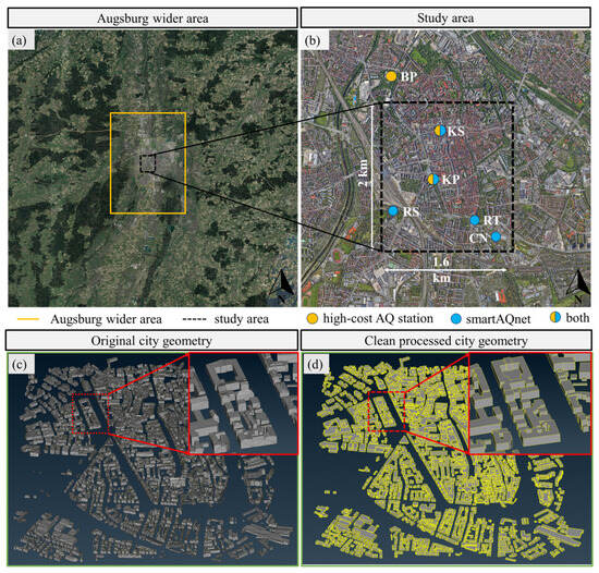
Figure 1.
Wider area of interest (a). Test case area containing smartAQnet sensors and official AQ stations (b). OpenStreetMap (OSM) representation of the city (c) and clean geometry of the urban area used for CFD modeling (d).
Accurately representing the geometric characteristics of the urban environment under study is crucial for effective air quality modeling using computational fluid dynamics (CFD) to provide precise representations of pollution levels and support accurate urban planning efforts [20]. To achieve this, the 3D geometry of the area of interest is obtained from OpenStreetMap (OSM), and processing is performed to clean and refine the surfaces of the buildings. This preparation is crucial when creating a digital grid on the designed area, smoothly incorporating the 3D model. Figure 1c shows the representation of the city from OSM (accessed December 2021) with a focus on specific buildings. Figure 1d shows the geometry used in this study after the cleanup process. This process was carried out by creating new 3D elements with the same geometrical characteristics as the OSM geometry. This step is performed with the use of ANSYS Spaceclaim 2018, a CAD software from the ANSYS package that is used for geometry creation and processing [17].
Figure 2a shows the digital domain of the urban area, confined within the density box. The computational domain’s height is set to 6Hmax, with an upstream distance of 15Hmax, where Hmax represents the tallest building’s height in the area, a chapel at 83.5 m [21], following established practices [22]. The labels N, E, S, and W correspond to the northern, eastern, southern, and western boundaries of the domain.
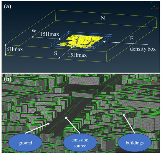
Figure 2.
Computational domain developed according to common practices (a). Focus on computational mesh developed on the buildings, ground, and emission sources (b).
A computational grid is developed that covers the digital model of the city using the ANSA commercial pre-processor. Focusing on an area containing the KP station, in Figure 2b, it can be seen that a surface mesh is developed on the buildings and ground’s surfaces. The rectangular objects shown also in Figure 2b at ground level represent the emission sources that are strategically positioned across main and smaller roads. Each emission source represents sections of roads where traffic activity releases pollutants into the surrounding environment. The purpose of the density box shown in Figure 2a is to include the area of the city and set a minimum grid size, in this case 4 m, to achieve the best refinement in the areas of interest included in the box, such as the emission sources and the buildings.
For this study, two computational grids are developed to examine their suitability. The volume mesh developed that covers all the domains for both grids uses tetrahedral unstructured elements with a growth rate of 1.2. The resolution on the buildings and the ground shown in Figure 2b is set at 1 m and on the emissions sources at 0.25 m for the medium-sized grid, allowing for high spatial accuracy of the CFD outputs with high refinement in areas near the emission sources and sensor locations. The parameter y+ indicating the quality of the grid at cells near to the wall is calculated for the ground and buildings at a value of 255 and 151, respectively, both within the range of 30–300 stated in the literature [23]. The medium computational grid consists of a total of 48 million elements, achieving the demanding accuracy for the convergence of the simulations for a 1.6 × 2 km2 urban area. The fine grid was developed with the same principle, with a resolution of 0.20 m on the emission sources and 0.8 m on the buildings. The total elements of the fine grid consisted of 72 million cells. The CFD simulations are performed on computer nodes with Intel(R) Core ™ i9-10980XE@3.00 GHz CPUs. Comparisons of the two grids indicated that the medium grid’s computational time was 19 h and the fine grid’s was 37 h, running on a total of 108 cores, both achieving scaled residuals of parameters of governing equations under the limit of 10−6 as proposed [24]. For computational purposes, the medium grid was selected for this study, given that it solves the cases two times faster and has also been used in other published studies [17,21].
2.2. Description of smartAQnet
As mentioned, this work aims to calibrate smartAQnet air quality network by integrating reference monitoring stations and a CFD model. The monitoring network is established in the city of Augsburg, Bavaria, and is composed of low-cost, mid-cost, and high-cost measuring devices. It was funded by the German Federal Ministry of Transport and Digital Infrastructure (BMVI), and it ran from 2017 until 2020 [16,19,25]. The backbone of the network are low-cost sensors called “Scientific Scouts”, which were developed as prototypes by the company GRIMM during the time of the project. The network monitors meteorological properties and aerosol concentrations with multiple sensors recording temperature, humidity, precipitation, and concentrations of PM10, PM2.5, and PM1 [25]. The temporal resolution of recordings ranges from minutes to hours. In the current work, all data were aggregated to hourly values. The KS, KP, and RT devices are placed in a traffic hot-spot area directly affected by vehicular activity, and the RS and CN provide urban background data. The network covers a total area of 16 × 16 km2 with a considerable number of sensors within a rectangular area of 6 × 4 km2, which covers urban and suburban areas of Augsburg [17].
During the development of the smartAQnet project, the first measurement phase in 2018 included using the “Scientific Scouts” EDM80NEPH sensors, developed by GRIMM. These nephelometric sensors were previously calibrated next to an EDM164 sensor that was used as a reference, also developed by GRIMM [19]. Local calibration demonstrated that one reference device can calibrate 5–10 scouts, with calibration frequency depending on site characteristics and pollution levels, and new PM algorithms were developed to account for environmental factors [26]. Another set of low-cost Nova Fitness SDS011 sensors was used in the project to measure PM that is considered to be of lower accuracy compared to the EDM80NEPHs. Budde et al. (2018) [27] examined the performance of the SDS011 sensors and stated that the devices do not capture PM10 satisfactorily if the size distribution of the particle measured changes, particularly if the distribution shifts towards larger particles. The sensors were then deployed in various positions throughout the urban area to begin the measurement campaign. More information about the architecture and development of the network can be found on the project website (www.smartaq.net).
In the period that this study focuses on, in September 2019, when traffic activity and more data to demonstrate this methodology was available, the readings of smartAQnet at RS, RT, and CN positions were given by newly installed optical counter devices (EDM80OPC). These new-generation devices, also manufactured by GRIMM, measure raw data across 24 size channels that range from 0.35 μm to 37 μm. The count data are then processed by an internal black-box algorithm to generate PM measurements. The sensors use equipment for measuring ambient and airflow temperature and humidity that their algorithm uses to adjust the PM predictions, which are translated into the smartAQnet readings that we use in this study. The added benefit of the approach introduced in this paper is that it provides adjustment at the point of their deployment to create new, more reliable datasets, combining CFD modeling and high-cost monitoring stations.
To tackle the inaccuracy of the network, attempts for re-calibration have been made in previous studies using gaussian processes to calibrate a set of Scientific Scouts and SDS011 sensors [13]. The re-calibration process involved using the monthly median of an official urban background station (BP) as a baseline, acknowledging potential under-calibration in traffic environments, and later comparing calibrated results with non-calibrated predictions to assess validity. The authors emphasized that the crucial factor for accurate predictions lies in individually calibrating the low-cost sensors according to their surrounding characteristics. Variability in pollutant concentrations across urban domains means that devices that are dispatched in various positions do not share the same reference, as meteorological and emission conditions vary. Capturing the demanded variability in pollutant concentration can be established with the use of CFD modeling [16]. This approach is followed here in this work by developing a spatially accurate air-quality model, incorporating dominant meteorological conditions, street emissions, and reference measurements to combine with low-cost sensors to create more reliable datasets.
2.3. Calibration Methodology
The calibration method employed in this study for smartAQnet is depicted in Figure 3. Initially, a CFD model is constructed using detailed traffic emissions and meteorological data, as elaborated in later Section 2.4 and Section 2.5. As a second step, the wind gradients produced by the CFD model are compared and validated against actual wind speed measurements within the studied area. Furthermore, we integrate reference urban background measurements with the simulated PM10 concentrations, and the modeled datasets are compared with readings from two official AQ stations located in KS and KP to assess the model’s performance in predicting pollutant concentrations. The validation process is thoroughly explained in Section 3.2. Upon validating the model and establishing its suitability, its modeled concentrations are used for calibrating the low-cost sensors.
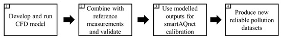
Figure 3.
Methodology followed to enhance smartAQnet PM measurements and to create more reliable PM concentration datasets.
This study takes a simple approach to calibrating the sensors. It compares their readings (a variable we want to adjust) with the produced pollutant concentrations (the variable we rely on) over a representative 24 h period. By performing linear fitting, we find a line that best aligns with the modeled data points used for calibration. The results of this approach are elaborated in Section 3.3 and Section 3.4.
2.4. Numerical Model
OpenFOAM (v2106), an open-source computational fluid dynamics (CFD) software, is used to simulate traffic-related pollutants in the surrounding urban environment. To produce the velocity field in the examined area, the modeling approach was based on the steady-state simpleFoam solver that uses the Reynolds-averaged Navier–Stokes (RANS) [28]. This solver is modified to encompass the passive-scalar transport equation to allow for pollutant dispersion [29]. Equation (1) denotes the advection–diffusion equation implemented in the solver. The term Deff represents the sum of the turbulent diffusion coefficient (Dt) and the molecular diffusion coefficient (Dm). Bonifacio et al. (2014) [30] performed particle dispersion simulation using CFD and concluded that the molecular term was 9 orders of magnitude smaller than the turbulent one. For that reason and because the test cases examined in this work concern low-wind speed conditions, where turbulent diffusivity is more dominant, Dm could be overall neglected in the simulations. Also, the mass conservation principle in the modeling approach can adequately predict PM concentrations over short distances, such as the distance between the road and the sensor [31]. This aligns with our study, as the emissions are close to the sensors, minimizing the chance of major coagulation phenomena during the simulation timeframe.
The k-epsilon turbulent model is employed in this study [32], as it is the most common used in urban applications of dispersion using CFD models, although it faces some limitations in terms of near-wall treatment and anisotropic flows. A review on common practices using CFD for pollutant dispersion applications examined the usage and suitability of turbulent models [24]. The authors explained that 78% of the cases used the k-epsilon model in all of their forms, including the realizable, RNG, and standard due to its robustness and computational efficiency in the RANS approach.
The computation of Dt relies on the turbulent Schmidt number (Sct) denoted in Equation (2), using the value Sct = 0.7 as proposed in the literature [33]. The turbulent viscosity term (vt) in Equation (2) derives from the atmospheric condition’s kinematic velocity and delineates the airflow characteristics at each timestep of the simulation. Each CFD steady-state simulation has a time resolution of one hour because the meteorological data as well as the high-cost measurements are given in hourly values. The inlets that are used for the introduction of air flow in the domain are the four boundaries that are shown in Figure 2a (N, E, S, W). The implementation of an ABL profile helps produce reliable wind fields in the domain, depicting accurately the wind profile observed in urban areas. Every simulation corresponding to the investigated hour used the measured wind characteristics shown in Figure 4(ai) for the 24 h period examined. The atmospheric boundary layer (ABL) profile is used in the inlets of the computational domain, as shown in Equation (3) [34]. In Equation (3), u* is the friction velocity, κ is the Von Karman constant, and z0 is the aerodynamic roughness length [35].
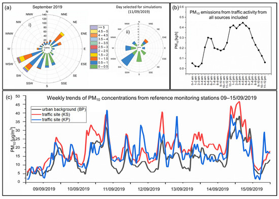
Figure 4.
Rose graph indicating wind direction and wind speed of September (ai) and for the day selected for simulations (aii) in Augsburg. Traffic originating PM10 emissions from all traffic sources included in the model (b). Demonstration of measured PM10 concentrations observed by reference monitoring stations between 9 and 15 of September (c).
In Table 1, the boundary conditions used in the CFD model are shown for three important parameters: velocity U, k, and epsilon. Depending on the wind direction, the condition atmBoundaryLayerInletVelocity is implemented in the inlet for U in the boundaries of the domain, and a fixedValue of k and epsilon is calculated based on the turbulent intensity (I), the turbulent length scale (l), and the inlet velocity (U). The condition for the outlet for velocity (U) is pressureInletOutletVelocity and inletOutlet for k and epsilon. In Table 1, it is also shown that for every parameter examined, the boundary condition on the top boundary was set at symmetry, as 44% of the cases found in the literature involving CFD for pollutant dispersion in urban areas use this constraint [24].

Table 1.
Boundary condition types used in the CFD model for inlets, outlets, buildings, emissions sources, ground, and top boundary for velocity (U), k, and epsilon.
2.5. Traffic Emissions and Meteorological Data
During September 2019, meteorological data indicated that the prevailing wind direction predominantly originated from the southwest, with an average speed of 0.83 m/s as shown in Figure 4(ai). The instrument responsible for observing these wind patterns is positioned on the southeastern side of the domain, specifically within the container area, and remains unaffected by the surrounding urban layout and buildings in the city center. To generate enough simulated data to showcase this methodology for calibrating the low-cost sensors, a comprehensive 24 h period is examined. Specifically, the selected day for this examination is Wednesday, 11th September 2019. This chosen day shares common characteristics with dominant wind conditions of September 2019, featuring southwest-directed winds with an average speed of 0.61 m/s (Figure 4(aii)).
In Figure 4b, the emissions during the examined 24 h period from all the emission sources included in the model show a typical weekday trend with morning and afternoon peaks. Within the digital model developed for this purpose, a setup of 69 emission sources has been integrated. The emission sources are strategically placed along major arterial roads and other smaller yet highly active roads within the area, ensuring a comprehensive traffic emission activity representation within the model.
Figure 4c shows the weekly trends of PM10 concentrations as indicated by the official AQ stations in the area. During the week between 9 and 15 September 2019, the two traffic sites at KS and KP had an average PM10 concentration of 20 μg/m3 and 16.6 μg/m3 and the urban background station at BP reported an average PM10 concentration of 14 μg/m3. On the selected 24 h period, the average PM10 concentration measured at KS, KP, and BP was 22 μg/m3, 18.9 μg/m3, and 15.8 μg/m3, respectively. These values indicate that the selected day is within the representative range of PM10 concentrations measured during that period, making it suitable as a test case for demonstrating the methodology applied in this work.
The setup of the emission sources shown in Figure 2b and explained in this section relies on specific road segments within the broader Augsburg area to capture traffic activity. These segments, identified as road IDs, constitute parts of the area’s roads. Detailed analysis conducted for the month of September has produced hourly deviations from the average daily traffic volumes (ADTV) for every individual ID. These deviations are used to produce a detailed traffic activity profile for urban conditions in the examined area, enabling a comprehensive temporal breakdown on an hourly basis [16]. PM10 is the pollutant examined, and it is selected because it is the only particulate matter pollutant that is observed by the official AQ stations in the area, to combine with the CFD results and to validate the model. Emission factors for PM10 from road traffic are calculated using the COPERT software (https://copert.emisia.com/), which is a European emission inventory model used to calculate air pollutants from road transport provided by EMISIA SA. The driving mode was selected at 50% urban peak and 50% off peak and an average speed of 30 km/h that indicates typical urban driving for various vehicle technologies. The Federal Motor Transport Authority provides information on the vehicle classification of the area of Augsburg examined for 2019, with 73.69% passenger cars, 12.45% light commercial vehicles, 7.49% motorcycles, 5.74% heavy duty trucks, and 0.63% buses. Using this information, a uniform emission factor for PM10 is used to calculate traffic emissions based on the number of vehicles and the length of the road for every hour.
3. Results and Discussion
3.1. Model Results
This section presents the outcomes of the CFD model regarding the modeled concentrations within the examined area. Figure 4b illustrates that the most severe traffic scenario, in terms of emitted mass, occurred between 16:00 and 17:00, with a prevailing wind direction from the southwest measured at 247 degrees. Hence, this scenario is chosen as representative for showcasing the CFD results in this section. All the simulations reached a level of residuals within the range of 10−6, indicating acceptable convergence as found in the literature [24]. Figure 5a depicts the location of the KS device on the northern side of the road at a height of 2.5 m, while the KP device (Figure 5c) is positioned at a 4 m height between two roads, capturing emissions from both east and west-bound traffic. Both stations are marked with a red dot. Figure 5b,d shows the respective locations on the model, along with the CFD-generated distribution of pollutant concentration. The corresponding point where the sensor is located in the digital model is indicated with a black dot.
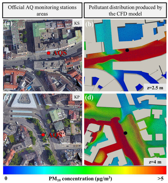
Figure 5.
Karlstrasse (KS) and Köningsplatz (KP) areas (a,c). Air quality stations depicted by the red dot. CFD pollutant concentration for KS and KP at the height of the sensors (b,d) and extraction points for AQS comparison depicted by the black dot.
This section highlights the CFD model’s high spatial resolution, which shows the assessment of pollutant variability at a street-scale level within the study area. By using the same modeling approach, within constrained areas at a street-canyon scale, differences of up to 68% in pollutant concentrations can be established [16]. Taking advantage of this, we are able to provide more representative pollution information on sensor locations. This precision is attained through turbulent modeling and fine mesh development, accurately portraying urban domain geometrical characteristics within the model [22], and can provide important information on the distribution of pollutants. This level of detail is a distinctive advantage of the CFD approach in air-quality modeling compared to Gaussian and Lagrangian models, enhancing the reliability of modeled concentrations in urban environments [36,37].
3.2. Model Validation
This section presents the model’s validation by comparing the model’s outputs with high-quality observed PM10 concentrations and wind speed data. Assessing the model’s performance against observations in the examined domain and period is crucial for the reliability of the modeled outputs. Figure 6a presents a comparison between modeled and observed wind speed values at the sensor point for wind field validation. There, it can be seen that the wind speed generated by the CFD model at that point appears to have lower values in the morning and night periods with distinguishable peaks during the mid-day period, the same trend observed by the measuring device. Figure 6b shows the regression analysis for both CFD and measured wind speeds, with a coefficient R = 0.87 and an average deviation of 7% during the day. Other studies also performed regression analysis with measured and modeled wind speeds to assess the performance of their CFD model, with deviations below 30% [38]. This analysis strongly supports the conclusion that the wind field produced by the CFD model is reliable, emphasizing the credibility of the model’s results.
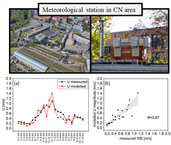
Figure 6.
Comparison between measured wind speeds and modeled ones (a) and regression analysis between modeled WS and meteorological station’s (b).
Two official air quality stations provide hourly concentrations of PM10 and are compared to the modeled PM10 concentrations. To directly compare modeled PM10 with measurements, urban background PM10 concentrations from Bourges-Platz (BP) high-cost AQ station (Figure 4c) for the selected period are added to the CFD-generated PM10 concentrations, considering that the background PM10 is distributed uniformly in the urban domain [39]. In Figure 7a,c, it is shown that the modeled PM10 concentrations follow the trends of the measurements for KS and KP, respectively. Peaks are observed during the morning period and late afternoon, and the average absolute daily deviation of the modeled pollutant concentrations from observations is 18% for KS and 13% for KP. Figure 7b,d shows the regression analysis performed for both stations. For KS, a correlation coefficient R = 0.96 and R = 0.86 for KP are established. The correlation coefficients calculated are within the accepted criteria of R > 0.8 found in the literature [40,41]. Statistical metrics for modeled results evaluation based on reference measurements are used for performance assessment, such as FAC2, FB, and NMSE [42]. These metrics are described in Equations (5)–(9) using normalized concentrations from observed (O) and predicted (P) values. Equation (4) describes how the normalized concentrations were calculated: C is the calculated concentration, Uref is the wind speed for every hour examined, Q is the emission rate, and H is the average building height of the study area, estimated at 15 m.
Factor of two (FAC2) counts the fraction of data points where the predictions are within a factor of two of the observations.
Fractional bias (FB) is a linear measure of the mean bias.
Normalized mean square error (NMSE) measures the scatter of the data.
Geometric mean bias (MG) is a logarithmic measure of the mean bias.
Geometric variance (VG) shows the scatter in the data and contains systematic and random errors.
Hit rate (q) specifies the fraction of model results that differ within an allowed range from comparison data.
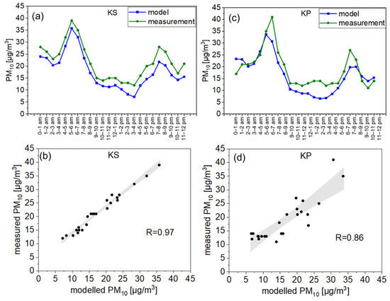
Figure 7.
Comparison between modeled concentrations and official measurements for Karlstraße (KS) (a) and Königsplatz (KP) (c). Regression analysis between model and measurement for KS (b) and KP (d).
For both reference stations, the modeled concentrations achieved a metric FAC2 between 0.91 and 0.96, FB between 0.08 and 0.23, and NMSE between 0.05 and 0.07. Any value above 0.5 is accepted for FAC2, below 1.5 for NMSE, and metrics calculated between −0.3 and 0.3 for FB also meet the criteria for acceptance as a validation of air-quality model performance against measurements [43,44].
Using reliable observations in the domain examined is crucial for drawing safe conclusions when applying air quality modeling. In this section, we showcased that during the examined 24 h period, which is taken to be representative of the meteorological conditions of September 2019, the wind field developed by the CFD model is accurate. The correlation between modeled and measured wind speeds in the area of observation shows an R = 0.87 and an average 7% deviation. Comparisons with PM10 concentrations at two high-quality AQ stations, showcased an average 15.5% deviation from modeled concentrations and indicated a shared correlation coefficient of R = 0.91. This outcome confirms that both the dispersion and the emission modeling approach used are accurate.
The model dataset produced is a combination of reference high-quality measurements given by the background station (BP) and high-resolution CFD modeling. The CFD model accounts for the street increment in the locations of deployed sensors. The accepted performance of the model’s results based on meteorological observations and high-quality PM10 concentrations supports the argument that it could be used in integration with low-cost air quality networks to produce more accurate pollution representation. The information that will be produced by using a combination of reference measurements, CFD modeling and indications of smartAQnet will provide more reliable concentrations of pollutants, that will benefit of the strength of measurements as top-down and high-resolution AQ modeling as bottom-up approaches. The application proposed in this work could be used to fill in missing values on low-cost sensors in case of malfunctions and to periodically calibrate their indications.
3.3. Comparison with smartAQnet Indications
The modeled concentrations are distributed in the examined digital domain and then compared to the indications of the smartAQnet sensors. These comparisons occur at the exact location and height, a benefit provided by the high spatial resolution of the CFD model. Figure 8a–c illustrates the contrast between the observed PM10 levels from the sensor network and the predicted modeled concentrations. The aim is to analyze and refine the smartAQnet readings using the model outputs. The best practice to assess the performance of the calibration would be to compare the calibrated datasets in KS and KP with the reference monitoring stations. During the period examined, when traffic activity data were available, the smartAQnet indications for KS and KP were the same as the official AQ concentrations measured at the corresponding areas. Any correction applied would just deviate from the reliable measurements given by the reference instruments, so the correction is only performed at RS, RT, and CN.
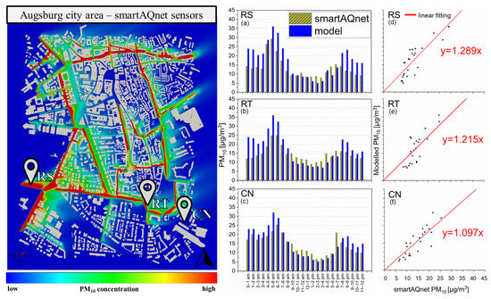
Figure 8.
Modeled concentrations vs. smartAQnet indications. Hour-to-hour comparison (a–c) and regression analysis with linear fitting to produce calibration equations (d–f).
Figure 8a–c depicts an underestimation in PM10 levels on RS, RT, and CN sensors by smartAQnet throughout the day, compared to the model. During the examined timeframe, the disparities between the RS, RT, and CN sensors’ readings and the modeled PM10 concentrations were evaluated. The CN sensor exhibited an overall average difference of 1 μg/m3, while the RS and RT sensors showed differences of 4 μg/m3 and 3 μg/m3, respectively on PM10 concentrations. On average, the absolute deviations from the reference modeled PM10 concentrations amounted to 23%, 15%, and 9% for the RS, RT, and CN sensors. Figure 8d–f presents regression analyses conducted for each sensor. The correlation factors (R) established for RS, RT, and CN were 0.83, 0.81, and 0.85, respectively. These correlation factors indicate that the trends observed by the sensors in terms of PM10 concentrations align with the values produced by the model, but there are differences in the levels of concentrations produced.
Linear fitting was employed to establish equations depicted in Figure 8d–f for the device’s calibration, using the modeled PM10 concentrations as targets. A linear fitting of y = ax was employed to correct for zero calibration, ensuring alignment of the sensor’s readings with reference values when it reads zero. In regression analysis, the slope (a) signifies the rate of change in the dependent variable y (model reference) per unit change in the independent variable (x) (low-cost sensor). An α > 1 indicates an underestimation of values by the low-cost sensors compared to the model’s dataset used for calibration. This discrepancy is also evident when comparing the indications of the three sensors (RS, RT, and CN) to those of the official AQ stations KS and KP. Figure 9a–c shows that the PM10 concentrations of the official stations KS and KP are higher than those of the smartAQnet sensors (RS, RT, and CN). The slope of the three sensors relative to the official stations during that time ranged from 1.118 to 1.694. Figure 8d–f reveals slopes of 1.289 for RS, 1.215 for RT, and 1.097 for CN compared to the modeled values, indicating the provided adjustment agrees with the official observations of PM10. This calibration method uses the advantages provided by the CFD model, as the values are given in the exact location of each sensor, so every calibration is unique, achieving more accurate reference. This consideration accounts for environmental characteristics such as wind intensity and turbulence influenced by surrounding buildings and local emissions of traffic PM10 emitted from nearby roads that differ from area to area.
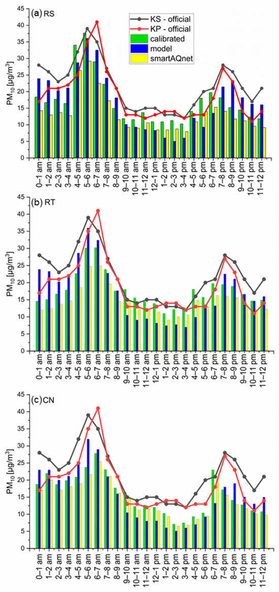
Figure 9.
SmartAQnet PM10 concentrations, modeled PM10 values, and calibrated PM10 dataset for RS (a), RT (b), and CN (c), respectively, and indications of high-cost measurements from KS and KP during the examined 24 h period.
3.4. Calibration of SmartAQnet Indications
The regression analysis in Figure 8 produced equations representing the relationship between sensor readings and PM10 concentrations. The calibration equations were then applied to correct the PM10 concentration dataset obtained from smartAQnet measurements, as depicted in Figure 9. In Figure 9a, the calibrated values from the RS sensor are shown with the original smartAQnet readings and the modeled values. Notably, the calibrated values exhibit a deviation of 1% from the modeled PM10 concentrations, an improvement compared to the previous 23%. Figure 9b,c illustrates the indications from the RT and CN sensors, respectively, showcasing daily deviations of 3% and 2% from the modeled dataset. The initial deviation of smartAQnet from the modeled dataset was 15% and 9%, respectively, for RT and CN.
To further demonstrate the impact of the calibration, the KS and KP PM10 concentrations from the high-cost monitoring stations are shown in Figure 9a–c. For the RS sensor, the calibrated dataset exhibited a deviation of 21% and 9% from the reference station in KS and KP, respectively, during the examined period, showcasing an improvement compared to the previous 39% and 30% daily deviation. In the case of RT, the new calibrated dataset deviated 19% and 6% from KS and KP, compared to the 33% and 23% deviation that the initial smartAQnet had. Finally, the CN calibration also exhibited improvement; as shown in Figure 9c, the calibrated dataset is closer to the KS and KP values compared to the initial one, demonstrating deviations of 27% and 16% from KS and KP, compared to the previous 34% and 24% daily average deviation. Overall, the calibration process has notably improved the alignment of sensor measurements with high-cost reference monitoring stations in the city and modeled values produced at the same points.
To assess the suitability of the calibration, statistical metrics that show the strength of the correlation between the corrected smartAQnet and the model are calculated after calibration. Table 2 shows the statistical metrics calculated for the linear fittings of smartAQnet for RS, RT, and CN when compared to the modeled results using dimensionless concentrations. These metrics are shown in Section 3.2. For RS, FB was reduced from the out-of-range 0.36 to 0.11. The HIT RATE calculated for every sensor was not acceptable before the calibration as it was lower than 0.66 [43], but after the correction brought it to an acceptable value. For all the cases, the calibration approach provided better statistical metrics that were closer to the ideal value. So, subsequently, the calibration applied to the sensors is determined to be suitable for calibrating the low-cost PM sensors, given that by applying the correction, a lower deviation from the model-target dataset and a better correlation with it are achieved. These metrics can be used to assess the performance of urban air quality networks and to indicate if there is an under- or over-prediction compared to target values. The new calibrated datasets created in the three locations of the low-cost sensors also exhibited a better correlation with the two high-cost reference monitoring stations, as explained in Section 3.4.
Table 2.
Statistical metrics between smartAQnet and calibrated datasets from modeled PM10 concentrations for RS, RT, and CN nodes.
4. Conclusions
This study proposed a method for calibrating low-cost sensor networks by combining reliable observations with modeled concentrations generated by computational fluid dynamics (CFD) modeling. The CFD model considers the examined area’s geometry and incorporates traffic emissions based on Augsburg’s traffic activity and fleet characteristics during the chosen period. The simulated 24 h period represents typical wind direction and speed for that month, ensuring representative results. The modeled PM10 concentrations exhibited high correlation (R = 0.97 and 0.86) with two official air quality stations, with deviations of only 18% and 13%, respectively. Similarly, the wind field showed strong agreement with observed data (R = 0.87, average daily deviation of 7%).
Regression analysis established correlation equations between modeled PM10 concentrations and sensor readings, enabling linear fitting calibration for each device. Applying this calibration to sensors requiring correction resulted in an average deviation of only 2% from target values. Statistical metrics like NMSE, FB, HIT RATE, and MG confirmed significant improvements in sensor-to-model value correlation, bringing them closer to ideal values. The new calibrated datasets exhibited a better correlation with two reference monitoring stations in the area, with reductions in deviation ranging from −7% to −21%. A limitation of this method is the exclusion of temperature and relative humidity, which can influence sensor performance [45]. Future research could incorporate all parameters affecting particle dispersion and all pollution sources for a more comprehensive air quality assessment and sensor calibration.
This method offers several advantages. It allows generating a database of modeled pollutant concentrations at various time scales under various meteorological and emission scenarios. The model’s results can calibrate sensors exhibiting systematic errors and fill in missing data caused by sensor malfunctions. The integration of cost-effective air quality networks, high-quality monitoring stations, and high-resolution air quality modeling leverages the advantages of both top-down and bottom-up approaches for comprehensive air quality assessment. Urban air quality networks can be used to assess the performance of air-quality models, and the modeling approaches can provide guidance on sensor installation and periodical calibration. By improving the accuracy and reliability of air quality data, this approach can enhance public health by enabling more effective pollution control measures. It can raise public awareness by providing communities with accessible, real-time information on air quality, empowering them to take proactive steps to reduce exposure to harmful pollutants in the frameworks of smart cities.
Author Contributions
Conceptualization, G.I., T.R. and L.N.; Methodology, G.I., P.T., C.L., T.R., N.R., C.B. and L.N; Software, G.I., N.R. and C.B.; Validation, G.I.; Formal analysis, G.I.; Investigation, G.I., N.R. and C.B.; Resources, G.I., P.T., C.L. and T.R.; Data curation, G.I., P.T., C.L. and T.R.; Writing—original draft preparation, G.I. and L.N.; Writing—review & editing, G.I. and L.N.; Visualization, G.I.; Supervision, T.R. and L.N.; Project administration, T.R. and L.N. All authors have read and agreed to the published version of the manuscript.
Funding
The research was funded by the Helmholtz Association of German Research Centres, through the GRACE foundation under funding number 51, in the frameworks of HEPTA project.
Institutional Review Board Statement
Not applicable.
Informed Consent Statement
Not applicable.
Data Availability Statement
Data are contained within the article.
Acknowledgments
Acknowledgements to the university of GRAZ for providing traffic information and the KIT for smartAQnet data. By using the CFD software we acknowledge OPENFOAM® as a registered trademark of OpenCFD Limited, producer and distributor of the OpenFOAM software v2106 via www.openfoam.com (accessed on 15 October 2021).
Conflicts of Interest
The authors declare no conflicts of interest.
References
- Piracha, A.; Chaudhary, M.T. Urban Air Pollution, Urban Heat Island and Human Health: A Review of the Literature. Sustainability 2022, 14, 9234. [Google Scholar] [CrossRef]
- Schwela, D.H.; Haq, G. Strengths and Weaknesses of the WHO Urban Air Pollutant Database. Aerosol Air Qual. Res. 2020, 20, 1026–1037. [Google Scholar] [CrossRef]
- Munir, S.; Mayfield, M.; Coca, D.; Jubb, S.A.; Osammor, O. Analysing the Performance of Low-Cost Air Quality Sensors, Their Drivers, Relative Benefits and Calibration in Cities—A Case Study in Sheffield. Environ. Monit. Assess. 2019, 191, 94. [Google Scholar] [CrossRef] [PubMed]
- Giordano, M.R.; Malings, C.; Pandis, S.N.; Presto, A.A.; McNeill, V.F.; Westervelt, D.M.; Beekmann, M.; Subramanian, R. From Low-Cost Sensors to High-Quality Data: A Summary of Challenges and Best Practices for Effectively Calibrating Low-Cost Particulate Matter Mass Sensors. J. Aerosol Sci. 2021, 158, 105833. [Google Scholar] [CrossRef]
- Raysoni, A.U.; Pinakana, S.D.; Mendez, E.; Wladyka, D.; Sepielak, K.; Temby, O. A Review of Literature on the Usage of Low-Cost Sensors to Measure Particulate Matter. Earth 2023, 4, 168–186. [Google Scholar] [CrossRef]
- Schmitz, S.; Towers, S.; Villena, G.; Caseiro, A.; Wegener, R.; Klemp, D.; Langer, I.; Meier, F.; Von Schneidemesser, E. Unravelling a Black Box: An Open-Source Methodology for the Field Calibration of Small Air Quality Sensors. Atmos. Meas. Tech. 2021, 14, 7221–7241. [Google Scholar] [CrossRef]
- Liang, L. Calibrating Low-Cost Sensors for Ambient Air Monitoring: Techniques, Trends, and Challenges. Environ. Res. 2021, 197, 111163. [Google Scholar] [CrossRef]
- Stavroulas, I.; Grivas, G.; Michalopoulos, P.; Liakakou, E.; Bougiatioti, A.; Kalkavouras, P.; Fameli, K.M.; Hatzianastassiou, N.; Mihalopoulos, N.; Gerasopoulos, E. Field Evaluation of Low-Cost PM Sensors (Purple Air PA-II) Under Variable Urban Air Quality Conditions, in Greece. Atmosphere 2020, 11, 926. [Google Scholar] [CrossRef]
- Frederickson, L.B.; Sidaraviciute, R.; Schmidt, J.A.; Hertel, O.; Johnson, M.S. Are Dense Networks of Low-Cost Nodes Really Useful for Monitoring Air Pollution? A Case Study in Staffordshire. Atmos. Chem. Phys. 2022, 22, 13949–13965. [Google Scholar] [CrossRef]
- Bisignano, A.; Carotenuto, F.; Zaldei, A.; Giovannini, L. Field Calibration of a Low-Cost Sensors Network to Assess Traffic-Related Air Pollution along the Brenner Highway. Atmos. Environ. 2022, 275, 119008. [Google Scholar] [CrossRef]
- Bagkis, E.; Kassandros, T.; Karatzas, K. Learning Calibration Functions on the Fly: Hybrid Batch Online Stacking Ensembles for the Calibration of Low-Cost Air Quality Sensor Networks in the Presence of Concept Drift. Atmosphere 2022, 13, 416. [Google Scholar] [CrossRef]
- Liang, C.J.; Yu, P.R. Assessment and Improvement of Two Low-Cost Particulate Matter Sensor Systems by Using Spatial Interpolation Data from Air Quality Monitoring Stations. Atmosphere 2021, 12, 300. [Google Scholar] [CrossRef]
- Paul, T.; Riedel, T.; Matthias, B. Spatial Interpolation of Air Quality Data with 616 Multidimensional Gaussian Processes. In INFORMATIK 2021, Proceedings of the Workshop Künstliche Intelligenz 618 in der Umweltinformatik (KIUI-2021), Berlin, Germany, 27 September 2021–1 October 2021; Gesellschaft für Informatik: Bonn, Germany, 2021; pp. 269–286. PISSN: 1617-5468; ISBN 978-3-88579-708-1. [Google Scholar] [CrossRef]
- Santiago, J.L.; Martín, F.; Martilli, A. A Computational Fluid Dynamic Modelling Approach to Assess the Representativeness of Urban Monitoring Stations. Sci. Total Environ. 2013, 454–455, 61–72. [Google Scholar] [CrossRef]
- Du, Y.; Blocken, B.; Abbasi, S.; Pirker, S. Efficient and High-Resolution Simulation of Pollutant Dispersion in Complex Urban Environments by Island-Based Recurrence CFD. Environ. Model. Softw. 2021, 145, 105172. [Google Scholar] [CrossRef]
- Ioannidis, G.; Li, C.; Tremper, P.; Riedel, T.; Ntziachristos, L. Application of CFD Modelling for Pollutant Dispersion at an Urban Traffic Hotspot. Atmosphere 2024, 15, 113. [Google Scholar] [CrossRef]
- Antoniou, A.; Ioannidis, G.; Ntziachristos, L. Realistic Simulation of Air Pollution in an Urban Area to Promote Environmental Policies. Environ. Model. Softw. 2024, 172, 105918. [Google Scholar] [CrossRef]
- Boikos, C.; Rapkos, N.; Ioannidis, G.; Oppo, S.; Armengaud, A.; Siamidis, P.; Tsegas, G.; Ntziachristos, L. Factors Affecting Pedestrian-Level Ship Pollution in Port Areas: CFD in the Service of Policy-Making. Build. Environ. 2024, 258, 111594. [Google Scholar] [CrossRef]
- Schäfer, K.; Budde, M.; Cyrys, J.; Emeis, S.; Gratza, T.; Grimm, H.; Hank, M.; Hinterreiter, S.; Pesch, M.; Petersen, E.; et al. Smart Air Quality Network for Spatial High-Resolution Monitoring in Urban Area; SPIE-Intl Soc Optical Eng: St Bellingham, WA, USA, 2018; p. 10. [Google Scholar]
- Trindade da Silva, F.; Costa Reis, N.; Santos, J.M.; Valentim Goulart, E.; Simões Maciel, F.; Bragança, L.; Engel de Alvarez, C. Atmospheric Dispersion and Urban Planning: An Interdisciplinary Approach to City Modeling. Sustain. Cities Soc. 2021, 70, 102882. [Google Scholar] [CrossRef]
- Gkirmpas, P.; Tsegas, G.; Ioannidis, G.; Vlachokostas, C.; Moussiopoulos, N. Identification of an Unknown Stationary Emission Source in Urban Geometry Using Bayesian Inference. Atmosphere 2024, 15, 871. [Google Scholar] [CrossRef]
- Blocken, B. Computational Fluid Dynamics for Urban Physics: Importance, Scales, Possibilities, Limitations and Ten Tips and Tricks towards Accurate and Reliable Simulations. Build. Environ. 2015, 91, 219–245. [Google Scholar] [CrossRef]
- Ariff, M.; Salim, S.M.; Cheong, S. Wall Y + approach for dealing with turbulent flow over a surface mounted cube: Part 1—Low reynolds number. In Proceedings of the Seventh International Conference on CFD in the Minerals and Process Industries, Melbourne, Australia, 9–11 December 2009. [Google Scholar]
- Pantusheva, M.; Mitkov, R.; Hristov, P.O.; Petrova-Antonova, D. Air Pollution Dispersion Modelling in Urban Environment Using CFD: A Systematic Review. Atmosphere 2022, 13, 1640. [Google Scholar] [CrossRef]
- Li, C.; Budde, M.; Tremper, P.; Schäfer, K.; Riesterer, J.; Redelstein, J.; Petersen, E.; Khedr, M.; Liu, X.; Köpke, M.; et al. SmartAQnet 2020: A New Open Urban Air Quality Dataset from Heterogeneous PM Sensors; Proscience: Culver City, CA, USA, 2021. [Google Scholar]
- Budde, M.; Riedel, T.; Schäfer, K. Mid-Term and 1st International Networking Workshop of the SmartAQnet Project December 4th and 5th 2018, Munich; Karlsruher Institut für Technologie (KIT): Karlsruhe, Germany, 2019. [Google Scholar] [CrossRef]
- Budde, M.; Schwarz, A.; Müller, T.; Schwarz, A.D.; Laquai, B.; Streibl, N.; Schindler, G.; Köpke, M.; Riedel, T.; Dittler, A.; et al. Potential and Limitations of the Low-Cost SDS011 Particle Sensor for Monitoring Urban Air Quality. ProScience 2018, 5, 6–12. [Google Scholar] [CrossRef]
- Peralta, C.; Nugusse, H.; Kokilavani, S.P.; Schmidt, J.; Stoevesandt, B. Validation of the SimpleFoam (RANS) Solver for the Atmospheric Boundary Layer in Complex Terrain. ITM Web Conf. 2014, 2, 01002. [Google Scholar] [CrossRef]
- Elfverson, D.; Lejon, C. Use and Scalability of Openfoam for Wind Fields and Pollution Dispersion with Building- and Ground-Resolving Topography. Atmosphere 2021, 12, 1124. [Google Scholar] [CrossRef]
- Bonifacio, H.F.; Maghirang, R.G.; Glasgow, L.A. Numerical Simulation of Transport of Particles Emitted from Ground-Level Area Source Using AERMOD and CFD. Eng. Appl. Comput. Fluid Mech. 2014, 8, 488–502. [Google Scholar] [CrossRef]
- Holmes, N.S.; Morawska, L. A Review of Dispersion Modelling and Its Application to the Dispersion of Particles: An Overview of Different Dispersion Models Available. Atmos. Environ. 2006, 40, 5902–5928. [Google Scholar] [CrossRef]
- Amorim, J.H.; Rodrigues, V.; Tavares, R.; Valente, J.; Borrego, C. CFD Modelling of the Aerodynamic Effect of Trees on Urban Air Pollution Dispersion. Sci. Total Environ. 2013, 461–462, 541–551. [Google Scholar] [CrossRef]
- Tominaga, Y.; Stathopoulos, T. Turbulent Schmidt Numbers for CFD Analysis with Various Types of Flowfield. Atmos. Environ. 2007, 41, 8091–8099. [Google Scholar] [CrossRef]
- Yang, Y.; Gu, M.; Chen, S.; Jin, X. New Inflow Boundary Conditions for Modelling the Neutral Equilibrium Atmospheric Boundary Layer in Computational Wind Engineering. J. Wind Eng. Ind. Aerodyn. 2009, 97, 88–95. [Google Scholar] [CrossRef]
- Irwan Ramli, N.; Idris Ali, M.; Saad, H. Estimation of the Roughness Length (zo) in Malaysia Using Satellite Image. In Proceedings of the Seventh Asia-Pacific Conference on Wind Engineering, Taipei, Taiwan, 8–12 November 2009. [Google Scholar]
- Boikos, C.; Siamidis, P.; Oppo, S.; Armengaud, A.; Tsegas, G.; Mellqvist, J.; Conde, V.; Ntziachristos, L. Validating CFD Modelling of Ship Plume Dispersion in an Urban Environment with Pollutant Concentration Measurements. Atmos. Environ. 2024, 319, 120261. [Google Scholar] [CrossRef]
- Toscano, D.; Marro, M.; Mele, B.; Murena, F.; Salizzoni, P. Assessment of the Impact of Gaseous Ship Emissions in Ports Using Physical and Numerical Models: The Case of Naples. Build. Environ. 2021, 196, 107812. [Google Scholar] [CrossRef]
- Ricci, A.; Janssen, W.D.; van Wijhe, H.J.; Blocken, B. CFD Simulation of Wind Forces on Ships in Ports: Case Study for the Rotterdam Cruise Terminal. J. Wind Eng. Ind. Aerodyn. 2020, 205, 104315. [Google Scholar] [CrossRef]
- Murray, D.R.; Newman, M.B. Probability Analyses of Combining Background Concentrations with Model-Predicted Concentrations. J. Air Waste Manag. Assoc. 2014, 64, 248–254. [Google Scholar] [CrossRef] [PubMed][Green Version]
- Jon, K.S.; Huang, Y.; Sin, C.H.; Cui, P.; Luo, Y. Influence of Wind Direction on the Ventilation and Pollutant Dispersion in Different 3D Street Canyon Configurations: Numerical Simulation and Wind-Tunnel Experiment. Environ. Sci. Pollut. Res. 2023, 30, 31647–31675. [Google Scholar] [CrossRef]
- Hang, J.; Liang, J.; Wang, X.; Zhang, X.; Wu, L.; Shao, M. Investigation of O3–NOx–VOCs Chemistry and Pollutant Dispersion in Street Canyons with Various Aspect Ratios by CFD Simulations. Build. Environ. 2022, 226, 109667. [Google Scholar] [CrossRef]
- Di Sabatino, S.; Buccolieri, R.; Olesen, H.R.; Ketzel, M.; Berkowicz, R.; Franke, J.; Schatzmann, M.; Schlünzen, K.H.; Leitl, B.; Britter, R.; et al. COST 732 in Practice: The MUST Model Evaluation Exercise. Int. J. Environ. Pollut. 2011, 44, 403–418. [Google Scholar] [CrossRef]
- Di Sabatino, S.; Buccolieri, R.; Pulvirenti, B.; Britter, R. Simulations of Pollutant Dispersion within Idealised Urban-Type Geometries with CFD and Integral Models. Atmos. Environ. 2007, 41, 8316–8329. [Google Scholar] [CrossRef]
- Goricsán, I.; Balczó, M.; Balogh, M.; Czáder, K.; Rákai, A.; Tonkó, C. Simulation of Flow in an Idealised City Using Various CFD Codes. Int. J. Environ. Pollut. 2011, 44, 359–367. [Google Scholar] [CrossRef]
- Gómez-suárez, J.; Arroyo, P.; Alfonso, R.; Suárez, J.I.; Pinilla-gil, E.; Lozano, J. A Novel Bike-Mounted Sensing Device with Cloud Connectivity for Dynamic Air-Quality Monitoring by Urban Cyclists. Sensors 2022, 22, 1272. [Google Scholar] [CrossRef] [PubMed]


Disclaimer/Publisher’s Note: The statements, opinions and data contained in all publications are solely those of the individual author(s) and contributor(s) and not of MDPI and/or the editor(s). MDPI and/or the editor(s) disclaim responsibility for any injury to people or property resulting from any ideas, methods, instructions or products referred to in the content. |
© 2024 by the authors. Licensee MDPI, Basel, Switzerland. This article is an open access article distributed under the terms and conditions of the Creative Commons Attribution (CC BY) license (https://creativecommons.org/licenses/by/4.0/).