Abstract
We compare three machine learning models—artificial neural network (ANN), random forest (RF), and convolutional neural network (CNN)—for spatial downscaling of temperature at 2 m above ground (T2M) from a 9 km ERA5-Land reanalysis to 1 km in a complex terrain area, including the Non Valley and the Adige Valley in the Italian Alps. The results suggest that CNN performs better than the other methods across all seasons. RF performs similar to CNN, particularly in spring and summer, but its performance is reduced in winter and autumn. The best performance was observed in summer for CNN (R2 = 0.94, RMSE = 1 °C, MAE = 0.78 °C) and the lowest in winter for ANN (R2 = 0.79, RMSE = 1.6 °C, MAE = 1.3 °C). Elevation is an important predictor for ANN and RF, whereas it does not play a significant role for CNN. Additionally, CNN outperforms others even without elevation as an additional feature. Furthermore, MAE increases with higher elevation for ANN across all seasons. Conversely, MAE decreases with increased elevation for RF and CNN, particularly for summer, and remains mostly stable for other seasons.
1. Introduction
Global climate models (GCMs) play a crucial role in predicting the state of the atmosphere [1]. However, these models’ spatial resolution is low, typically between 25 and 100 km, because of computational limitations. Such a spatial resolution is suitable for analyzing large-scale features, e.g., synoptic or mesoscale processes, but too coarse for capturing the spatial variability of meteorological parameters in complex terrain [2,3]. This limits the straightforward use of GCM output for decision-making processes.
The near-surface air temperature of Earth is an essential parameter for a series of processes, especially for terrestrial life, including that of humans and the ecosystem. In particular, the air temperature measured 2 m above the ground (T2M) is a standard reference variable adopted to represent processes relevant to various sectors like agriculture and transportation. The high-resolution daily mean temperature data can also have applications in various studies, such as those dealing with urban heat islands and thermal comfort. The interaction between surface temperature and urban morphology can be explored in greater detail by utilizing high-resolution temperature data [4]. Similarly, daily mean temperature can help study landscape interventions, such as the effect of increased vegetation on thermal conditions [5]. For these applications and to better predict these processes, there is an increasing need for high-resolution T2M datasets. Two main types of downscaling techniques are used to evaluate data from coarse resolution to local scale, i.e., dynamic and statistical downscaling. Dynamic downscaling techniques use regional climate models to simulate physical processes by assuming initial and boundary conditions from GCM output. Fine-scale processes are represented with more accuracy, thus improving the provision of local-scale data [6,7]. However, dynamic downscaling usually requires considerable expertise and computational resources. Instead, statistical downscaling stems from a statistical relationship between large-scale climate variables (predictors) and local-scale variables (predictands) [8]. These relationships are exploited to predict values of the local-scale variables at different times and locations. Statistical downscaling techniques have an advantage in reduced computation and more straightforward implementation and thus are widely used in applications related to climate change [9,10,11].
Machine learning (ML) techniques have been increasingly used in recent years for statistical downscaling of daily mean temperature because of their ability to capture patterns within complex data. Various studies have employed different ML models, such as linear regression [12], support vector regression (SVR) [13,14], artificial neural network (ANN) [9,15,16], random forest (RF) [9], and k-nearest neighbor (KNN) [10] for downscaling temperature.
The ANN model is inspired by the human brain and consists of neurons with different layers. The input layer is the first layer, and, as the name suggests, it provides input data to the model; then comes the hidden layer, with one or more layers responsible for the model performance. The last is the output layer, where we obtain a prediction of the model. ANN can capture nonlinear relationships between parameters, making it useful for complex tasks such as downscaling temperature.
RF constructs multiple decision trees and takes the ensemble mean of outputs of all trees for final prediction. Gradient boosting (GB) is also an ensemble method that builds models sequentially. Each new model in GB corrects the errors of the earlier one. Both RF and GB leverage the strengths of multiple individual models to improve prediction accuracy, albeit through different mechanisms.
The MLR model uses a linear equation to capture the relationship between the predictor and predictand parameters. SVR aims to find a hyperplane that fits the data, making it suitable for capturing nonlinear temperature patterns. The KNN model predicts the value of a location depending on the values of its nearest neighbors in the dataset.
In the past, several studies have compared ML techniques for downscaling purposes. Pang et al. [9] conducted a study in the Pearl River Basin (Southern China) using three methods, namely multiple linear regression (MLR), RF, and ANN, to downscale mean temperature data from coarse resolution. Their study revealed that RF exhibited superior performance compared to both ANN and MLR. Azari et al. [10] used six different models—MLR, KNN, ANN, RF, SVR, and adaptive boost—in daily mean temperature downscaling at Memphis International Airport (USA). The results showed that ANN outperformed other models. Hanoon et al. [17] demonstrated that neural networks outperformed GB, RF, and linear regression in predicting daily temperature in Terengganu state (Malaysia). Hence, the literature suggests that no model can be considered invariably superior when comparisons are made across diverse regions. This emphasizes the need for conducting intercomparison studies specifically suited to where downscaling applications are required. However, it should be noted that most of these studies have employed ML techniques to downscale the daily mean temperature on a point scale. This approach involves taking low-resolution data from the closest grid point of the weather station for downscaling. Hutengs and Vohland [18] used RF for downscaling of LST spatially from 1 km to a resolution of 250 m in Jordan River Valley. However, the application of these techniques for spatial downscaling of the daily mean temperature is limited.
Recent studies on the downscaling of atmospheric variables have explored the application of a convolutional neural network (CNN). CNN models are similar to ANN models; however, in addition to fully connected dense layers, CNN consists of a few more layers, such as convolution and pooling layers. CNNs are especially effective for handling gridded data, such as spatial data or images. CNN models have gained increasing popularity for downscaling spatial gridded data, considering their ability to capture spatial features effectively. Bano Medina et al. [19] conducted a study in Europe with the objective of intercomparing CNNs of different complexity with linear models, bringing the horizontal resolution from 2° to 0.5° both for latitude and longitude. Their findings suggest that CNNs perform better compared to linear models, particularly as downscaling was performed on a continental scale, considering a large area, and with a relatively low scaling ratio. (The scaling ratio is calculated as the predictor resolution divided by the target or predictand resolution.) Therefore, the transferability of these results to a higher resolution remains unanswered.
Mountainous terrains are known to exhibit a variety of climatic situations [20] with very different features compared to surrounding plain areas nearby [21]. Accordingly, peculiar boundary layer processes occur therein, deeply affecting surface–atmosphere exchanges and, hence, surface temperatures, resulting from a variety of combinations of different land forms, ambient conditions, and surface properties [22]. In particular, under weather characterized by wide and persistent anticyclonic situations typically associated with clear skies and calm wind at the synoptic scale, daily-periodic, thermally-driven wind systems are generated by the regular cycle of surface heating and cooling [23]. Enhanced heating and cooling are both favored by clear skies, allowing for both strong incoming solar radiation during daytime and strong radiative loss during nighttime, respectively [24,25]. Under the different phases characterizing these winds, air typically flows up the slopes during daytime and downslope during nighttime, with transitional reversals at sunset and sunrise, respectively [26]. These factors affect surface temperature, particularly at the floor of valleys and basins, where long-lasting, ground-based temperature inversions and persistent cold pools often occur [27] fed by katabatic winds flowing down from the surrounding sidewall slopes [28].
Given such variability arising from a nontrivial combination of factors, downscaling is a particularly challenging task over mountainous terrain. On the other hand, the availability of high-resolution T2M is critical for a series of applications [29], ranging from air pollutant transport [30,31] to water resource management to agriculture. Hence, high-resolution data from NWP models were obtained with smoothing topography for computational stability [32]. Smoothing the topography can lead to a less accurate representation of the terrain affecting local atmospheric processes. However, ML models can leverage high-resolution data, overcoming these limitations to provide more accurate forecasts. Mutiibwa et al. [33] investigated the relationship between air temperature near surface and land surface temperature (LST) in mountainous terrain. Their study found that the LST serves as a reliable proxy for air temperature near the surface, with higher accuracy in the daytime compared to the nighttime. Li et al. [34] evaluated machine learning model performance for downscaling the LST, highlighting the better performance of machine learning algorithms compared to traditional regression approaches. Wang et al. [35] used CNN to downscale the daily temperature from their different coarser resolutions (100, 50, and 25 km) to a fine resolution (4 km), with better results obtained for downscaling from 25 km. Their study achieves good results with a scaling ratio of 6. However, 4 km is still very coarse for areas of complex terrain. Sha et al. [3] conducted a study over complex terrains in the western United States to lower the temperature from 0.25° (approximately 27 km) to a resolution of 4 km using CNN and found a higher MAE in mountainous areas and a lower MAE in the plains. Furthermore, when developing a model for downscaling temperature in complex terrains, the selection of predictors is crucial. For example, Karaman and Akyurek [36] conducted a study in Turkey, aiming to downscale the daily mean temperature on station data using an RF model, and found that incorporating static features such as elevation as additional predictors significantly improved the model’s performance. Some studies have included dynamic parameters such as dew point, pressure, and wind speed as additional predictors to improve the performance of the model [10,17]. Sebbar et al. [37] downscaled hourly temperature using SVR, XGBoost, and MLR by incorporating environmental lapse rate for temperature corrections. However, this study has limitations in regions where there is an unavailability of temperature data at various vertical levels. Therefore, our study employs ANN, RF, and CNN advanced neural networks to capture spatial and temporal variability directly from surface data.
This study presents various novel contributions to atmospheric research, especially in the field of spatial downscaling. The objective of the study presents a comprehensive intercomparison of the machine learning algorithms’ performances, namely ANN, RF, and CNN, in downscaling spatial daily mean temperature. While proposed models have been individually employed in downscaling studies, our work is novel in rigorously comparing their performance at high resolution and in complex terrain settings. Our study achieves a higher downscaling ratio (9), which is a significant leap compared to earlier studies [19]. This study places a strong emphasis on assessing the importance of elevation using a sensitivity experiment by providing elevation as an additional input. Here, we understand how different models respond to elevation as an additional input and improve the performance of models. We conduct a feature importance analysis showing key predictors that primarily contribute to enhancing model performance in different seasons. Furthermore, this is one of the first attempts at daily mean temperature downscaling in the Non and Adige Valleys, a region with very complex terrain in northern Italy, using machine learning.
Spatial downscaling often encounters constraints due to the unavailability of high-resolution predictand or target datasets, which can limit the scope of such studies. Instead, our research benefits from a gridded 1 km dataset for daily mean temperature created using ground-based measurements [38], providing a unique opportunity to explore spatial downscaling at high resolutions in this area.
The paper is organized as follows. Section 2 describes the materials and methods, including the study region, the datasets used, and the methods adopted. Section 3 describes the ML models employed in the study. Section 4 presents the results, which include the spatial consistency of models, average metrics of model performance, spatial and seasonal variation in model performance, sensitivity of models to elevation, and feature importance. Section 5 provides a discussion of the results, and Section 6 draws some conclusions and presents an outlook on possible future developments.
2. Materials and Methods
2.1. Study Region
Trentino-Alto Adige/South Tyrol is a mountainous region in the southern part of the European Alps in northeastern Italy. The region covers an area of around 13,000 km2. Our study focuses on an area including part of the Non and Adige Valleys, marked in a rectangular box in Figure 1. The region is complex enough to challenge the models. The topography of the area exhibits elevation ranges from 166 m to 2628 m ASL, with rather narrow valleys and steep slopes. The elevation distribution histogram for both the Non Valley and the Adige Valley shows a strongly varied terrain with a significant concentration of elevations in the range 500–1400 m, but fewer points exhibit higher elevations, especially above 1700 m (Figure 2).
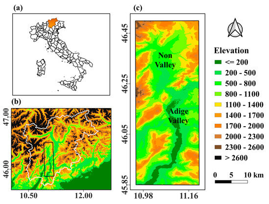
Figure 1.
(a) Position of Trentino and South Tyrol in Italy. (b) Orography of Trentino and South Tyrol. (c) Non Valley and Adige Valley.
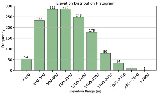
Figure 2.
Elevation distribution of the grid points in the study area, including the Non Valley and the Adige Valley.
The climate of the region is typical of a transition area between central Europe, with continental weather dominated by Atlantic influences, and a temperate Mediterranean area influenced by the sea; however, the area is also undergoing increasingly frequent outbreaks of the African anticyclone during summertime [38,39,40]. The region is renowned for agriculture, particularly for apples, grapes, and berries [41]. These agricultural activities play an important role in the economic prosperity of the region. Additionally, Trentino-South Tyrol is famous in terms of tourism and various sports activities, such as ski-mountaineering and hiking [42]. Therefore, understanding temperature dynamics in this distinctive landscape is important for increasing agricultural productivity and having sustainable tourism to strengthen economic development.
The climatology of the target area exhibits variations in temperature patterns across the seasons. The main climatological statistics of the area were calculated over the Non and Adige Valleys, spreading from 45.85° to 46.49° latitude and from 10.95° to 11.19° longitude using a comprehensive dataset of daily mean temperature available from 1980–2018 (Crespi et al. 2021) [38]. The region experiences a maximum daily mean temperature that reaches 22 °C and a minimum daily mean temperature of up to 8 °C in summer. On the other hand, during winter, there was a maximum daily mean temperature of 3.4 °C and a minimum daily mean temperature that plunged to −5.9 °C.
As outlined above for all mountainous areas, in this region too, surface temperatures are affected by a variety of factors associated with terrain complexity. In particular, the target area is known to develop regular valley wind systems [43,44,45] associated with peculiar boundary-layer turbulent exchanges. Also, the frequent occurrence of snowfalls and the persistence of snow cover during winter and spring in many parts of the domain also affect the surface temperatures.
2.2. Datasets
In this section, datasets used in the study are discussed. An overview of the different datasets used in the study can be found in Table 1.

Table 1.
Datasets used in the study.
- ERA5-Land
ERA5-Land is the reanalysis provided by the European Centre for Medium-range Weather Forecasts and consists of hourly data with a spatial resolution of 9 km (0.1° × 0.1°). The dataset is available from January 1950 to the present. For this study, hourly data from 1980 to 2018 over the Non and Adige Valleys were used. The primary predictor adopted for this study is the ERA5-Land T2M daily mean temperature (ERA5L-T2M). In addition, other auxiliary predictors used are dew point temperature at 2 m AGL (D2M), surface pressure (SP), zonal (U10) and meridional (V10) components of wind at 10 m AGL, surface net solar radiation (SNR), surface latent heat flux (SLHF), sensible heat fluxes (SSHF), snow cover (SC) area fraction, and wind speed (WS) at 10 m AGL.
- Reference Target Gridded Daily Mean Temperature Data
The target or predictand dataset for this study is the gridded fine resolution dataset of daily mean T2M. The daily dataset is available from the period of 1980–2018 over the Trentino and South Tyrol region. The dataset is created using more than 200 meteorological stations with a gridded resolution of 250 m × 250 m using interpolation techniques [38]. We aggregated 250 m resolution data to 1 km, which serves as a target for the study.
- Digital Elevation Model Data
The digital elevation model (DEM) used in the study was obtained from the Shuttle Radar Topography Mission (SRTM) of the National Aeronautics and Space Administration (NASA). The DEM covers the entire Earth’s surface, providing elevation information with a 30 m spatial resolution. For the purpose of the present study, the elevation data were spatially aggregated by averaging 33 × 33 pixel blocks, resulting in a 1 km resolution to match the pixel or grid size of the target data.
2.3. Methods
In this study, we adopted three ML algorithms: ANN, RF, and CNN. The choice of these models for this study is supported by earlier research that showed the strong performance of these machine learning models for downscaling temperature. Various intercomparison studies showed the effectiveness of ANN and RF models in capturing complex nonlinear relationships between different input features and target temperatures. For example, as explained above, Azari et al. [10] compared six different ML models, including MLR, KNN, ANN, RF, SVR, and adaptive boost, and found that ANN showed superior performance over other models. Similarly, Pang et al. [9] found that the RF model performed better than ANN and MLR in downscaling mean temperature over the Pearl River basin. In another study, Hanoon et al. [17] found that ANN outperformed other models, such as gradient boosting, RF, and linear regressions, for predicting daily temperature in Malaysia. These findings from several intercomparison studies helped us select the models ANN and RF for spatial downscaling tasks. In addition to this, CNN was selected as another model for our study, as it has been used in various spatial downscaling tasks due to its ability to understand spatial features from datasets [3,19,35].
We re-projected the target data to normal lat-lon projections from the Universal Transverse Mercator projection using the Pyproj library in Python to align with the ERA5-Land data. Also, we aggregated hourly data from ERA5-Land to a daily time scale using the resample function of the xarray library in Python. Our goal is to identify the best-performing model along with a downscaling ratio that is sufficiently moderate but possibly higher than in earlier studies [19]. Thus, the high-resolution datasets’ temperature and elevation are upscaled to 1 km using interpolation techniques. In principle, different interpolation techniques may lead to differences in results. In this study, we tested two interpolation techniques, namely, the nearest neighbor and averaging methods. In fact, we observed that differences in interpolated or upscaled datasets may occur, but they are mostly negligible. In particular, the nearest neighbor method preserves original values by allocating the nearest grid point value, and it may result in abrupt changes in temperature or elevation in complex terrain. This method preserves original values without smoothing, so it is particularly suited for categorical values. On the other hand, in the averaging method, grid values are calculated by averaging neighboring grid points and provide a smoother and more consistent transition between grids; this method is therefore suitable for continuous variables such as elevation and temperature. Therefore, we opted for the averaging method to interpolate our datasets. The high-resolution dataset of 250 m was spatially aggregated by averaging 4 × 4 pixels, resulting in a 1 km resolution, which serves as the target data. The DEM data at 30 m spatial resolution was also upscaled to 1 km by averaging over 33 × 33 pixels using spatial aggregation blocks to match the target grid resolution. The predictors from ERA5-Land were re-gridded to match the shape of the target data by keeping the resolution of 9 km the same as in earlier studies [8,46].
In addition, we derived a few more static features from the DEM, such as slope, aspect, cross-sectional curvature (C-curv), and longitudinal curvature (L-curv), in order to obtain more auxiliary predictors [47,48]. The schematic of these features is shown in Figure 3. The slope was evaluated as the first-order derivative of elevation and represents the local steepness of the surface. The aspect represents the direction that the slope faces. The curvature measures the rate of change of the slope and shows the concavity or convexity of the terrain; it is evaluated from the second-order derivative of elevation. The curvature of the surface, which is perpendicular to the direction of the slope, is called the C-curv, whereas the curvature along the direction of the slope is called the L-curve. All these features are derived using QGIS.
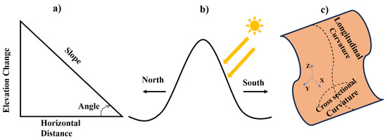
Figure 3.
Schematic for static features derived from elevation, including: (a) slope, (b) aspect, and (c) longitudinal and cross-sectional curvatures (L-curv, C-curv).
ML models have been created separately for each month to obtain better performance considering the seasonal temperature variation. For ANN and CNN, standardization of input features was carried out by subtracting the mean and dividing by standard deviation to have zero mean and unit standard deviation [49]. This process of rescaling the features to a comparable scale helps in achieving faster convergence during training [16,50]. Without standardization, features or predictors with higher values can dominate the training process, potentially leading to longer convergence times. On the other hand, RF does not require standardization, as decision trees used in algorithms are not affected by the scale of input features. In this study, we aim to downscale ERA5-Land T2M from a spatial resolution of 9 km to 1 km, thus having a downscaling ratio of 9.
The ERA5-Land input features that have a good correlation with target temperature are selected in this study based on previous downscaling studies [9,16]. These studies have shown that the features that have a high correlation coefficient with the predictand are effective predictors in downscaling. Also, the addition of each feature to the model training process for the ANN and RF models was conducted in a step-wise manner. In the beginning, T2M is used as a single predictor in order to have a baseline performance. Then, additional predictors are included one at a time to evaluate their contribution to the model’s performance. This iterative method enables a careful, incremental evaluation of each predictor’s impact, retaining only those contributing to improving the model performance. For ANN and RF models, we observed a gradual improvement after the systematic addition of 15 predictors. This includes dynamic features such as ERA5L-T2M, U10, V10, WS, SP, SC, SSHF, SLHF, and SNR, along with static features such as elevation, slope, aspect, C-curv, and L-curv. A similar approach was adopted for CNN, starting with ERA5L-T2M as the only predictor for baseline performance. However, incrementally testing additional predictors such as slope, aspect, C-curv, and L-curv, along with the dynamic feature SC, was observed to adversely affect the model, thereby degrading its performance. We performed a sensitivity study for January with a combination of static and dynamic features to evaluate their impact on the performance of the model using the RMSE, MSE, and R2 metrics. A detailed performance analysis of different feature combinations using these metrics can be found in Supplementary Materials. Based on this analysis, we found that dynamic features such as U10, V10, and wind speed contributed positively to model performance, whereas static features such as slope, aspect, and curvature degraded the performance of the model. We diagnosed that the inclusion of these static features might have acted as noise, leading to the lowered performance of the model. Therefore, these features were systematically excluded, leading to a formulation set of 10 predictors for the CNN model.
We used a temporal split of the dataset for evaluating models instead of traditional k-fold cross-validation. For time series data, the temporal split is useful in assessing the model’s ability to generalize with future unseen data. In particular, the daily datasets spanning from 1980–2018 are split into two parts: the training period from 1980–2009 and the testing period from 2010–2018. The proposed models in the study are compiled using mean squared error (MSE) as a loss function. MSE is selected for its ability to penalize large errors more severely, making it a good fit for temperature downscaling, as temperature data can exhibit sharp variation over short distances, especially in complex terrains. In the MSE loss function, errors are squared, thereby punishing larger deviations between predictions and observed temperatures. Other loss functions such as MAE measure average magnitude errors. Also, MAE treats all errors equally, meaning it is less sensitive to large errors and therefore less effective in addressing sharp temperature gradients in complex regions. Therefore, we chose MSE as our loss function for models, as it is widely used in different regression tasks [51,52]. As customary in forecast verification procedures, the performance of the models is analyzed from the metrics: correlation coefficient (r), root mean square error (RMSE), mean absolute error (MAE), coefficient of determination (R2), and mean bias error (MBE) [51]. The correlation coefficient (r) is used to measure the linear relationship between the model’s predicted and observed values. RMSE gives more weight to large errors, since it squares errors before averaging. This makes it sensitive to outliers. MAE allows for quantifying average error in predictions across the study area. It is calculated as the average of the absolute difference between the model’s predicted and observed values. R2, also called the coefficient of determination, is used to quantify the proportion of the variance in the dependent or target variable that is predictable from the independent variables. R2 can have values that range from 0 to 1. The MBE is used to capture average bias in model prediction by calculating the mean difference between the model’s predicted and observed values. MBE considers the direction of errors, and it ranges from to , with values close to 0 considered best. The evaluation metrics and their formulas are summarized in Table 2 below.
Table 2.
Evaluation metrics with their formulas.
Here, n represents the number of observations, represents model predicted values, represents observed values, represents mean model predicted values, represents the mean of the observed values, and y is any variable (e.g., temperature).
To understand the significance of elevation in model performance, we performed a sensitivity study. First, we trained the models using ERA5L-T2M as the only predictor, and secondly, we trained models by giving ERA5L-T2M and elevation (EL) data as predictors. We then evaluated the performance of models with and without elevation using correlation (r) and R2, values along with a scatter density plot. The feature importance for the ANN model was calculated using Shapley Additive Explanations (SHAP) to understand the role of each feature in model prediction [53]. SHAP gives importance to each feature for a given prediction, which provides a way to explain the output of ML models. We calculated SHAP values for each feature of the ANN model using the SHAP library in Python. For the CNN models, permutation importance was computed by perturbing each feature in validation data and measuring the change in model performance [54]. The permutation importance assesses the impact of the feature by measuring changes in the performance of the model when feature values are randomly shuffled. Lastly, for RF, the intrinsic feature of RF algorithms directly gives the feature importance without the need of additional methods such as permutation or SHAP required for ANN and CNN.Feature importance for all models was calculated for months and then aggregated over seasons for analysis. The values of feature importance were normalized to between 0 and 0.5 for a consistent and meaningful comparison between models.
3. Models Used in the Study
In this section, we briefly describe the three ML models, namely ANN, RF, CNN, along with their architecture.
3.1. Artificial Neural Network (ANN)
In this study, a feed-forward neural network with three layers is employed for the downscaling task. To identify the architecture for the ANN model with optimal performance, we conducted sensitivity experiments. We trained and tested different configurations with different numbers of neurons in the input and hidden layers, changing network depth to identify the best balance between model accuracy and complexity. After this sensitivity study, we found that the configuration (15-48-1) with 15 neurons in the input layer, 48 neurons in the hidden layer, and 1 neuron in the final output layer, performed best while avoiding unnecessary complexity. The rectified linear unit (ReLU) is used as an activation function in the hidden layer, and the Adam optimizer is used to optimize the neural network. The final layer is a single neuron output with a linear activation function aptly chosen for the regression task. The model is trained for 300 epochs using early stopping, which is used to monitor the loss and stops the training when no improvement is observed after the patience parameter of 10 epochs. The batch size for model training was set to 512 after a series of experiments with batch sizes to enhance training accuracy. The ANN model is provided with 10 dynamic features and 5 static features. The ANN model performed best with this set of predictors.
3.2. Random Forest (RF)
RF is an ensemble of decision trees used for both regression and classification tasks. The RF technique was first developed by [55] in 2001. RF constructs multiple decision trees during training, and every tree is trained on a different dataset subset. Each tree produces its output, and the final output of the RF model for the regression problem is the average of the prediction of all trees [9]. The averaging method increases the accuracy by reducing variance in error and by reducing overfitting. The robustness of the RF model in handling complex datasets and capturing nonlinear relationships makes it effective for identifying patterns in datasets and making accurate predictions in regression problems. RF is provided with 10 dynamic features and 5 static features. We tested the RF model with estimators or trees ranging from 50 to 100 to obtain the optimal performance. We observed that the time required by the model for training and prediction increases as the number of estimators increases. The RF model performed best with 100 estimators, ensuring optimal performance for our downscaling task. The random state parameter is set to 42 to ensure reproducibility of the results across different runs. The default values for the other parameters performed adequately for our task.
3.3. Convolutional Neural Network (CNN)
A CNN is a type of ANN built for processing grid-like data, such as images [56,57]. In addition to the layers present in ANN, CNN models have a couple more layers known as the convolution layer and pooling layer. The convolution layer consists of filters, also known as kernels, that slide over input data, calculating element-wise multiplication and summations. This process extracts features such as edges or textures from input data. After the convolution layer, we have the pooling layer in CNN. The role of the pooling layer is to decrease the spatial dimension of the feature maps produced by the convolution layers. In this study, we have used the max-pooling technique [58]. After two convolution and pooling layers, two fully connected dense layers are used for final predictions. We used the ReLU activation function to bring nonlinearity into the network [52]. In this study, we designed a CNN model with 2 convolution layers with 16 filters in the first layer and 32 filters in the second layer. Each convolution layer uses a kernel size of 3 × 3. This configuration was selected after a series of experiments with filter size and number of filters. The max pooling layer with a 2 × 2 size was applied after the convolution layer. We tested different neuron configurations after the flattening operation in the dense layer and found the best performance with 256 and 128 neurons in this setup. The CNN model was trained for 300 epochs, with early stopping applied and with patience parameters of 10. The architecture for the CNN model used in this study is shown in Figure 4.
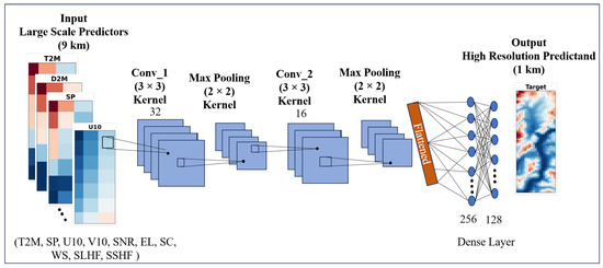
Figure 4.
Architecture for the CNN model with different layers. From the left at the first level, there is the input layer where input predictors are provided. Then, there comes a pair of convolution layers and a max pooling layer. The first convolution layer has 32 filters and the second 16 filters, both having a kernel size of 3 × 3. The max pooling layer with kernel size is 2 × 2. The last layers are fully connected dense layers with 256 and 128 neurons, respectively.
4. Results
In this section, we show the results of downscaling in terms of the consistency of models in predicting T2M, comparison of models using aggregated metrics, spatial and seasonal variation in the performance of models, and the importance of elevation for the models using sensitivity and feature importance.
4.1. Spatial Consistency of Models
We selected representative days for each season to evaluate the spatial consistency of machine learning models in predicting T2M: for winter (15 January 2015), spring (15 April 2015), summer (15 July 2015), and autumn (15 October 2015) (Figure 5). In the figure, Input-T2M is the input ERA5L-T2M with a coarser resolution of 9 km. ANN, RF, and CNN represent the downscaled T2M output of respective models at a spatial resolution of 1 km, whereas Crespi represents target reference T2M with a spatial resolution of 1 km. The selection of days was based on the typical seasonal characteristics. The primary goal here was to visually assess whether the proposed models can reproduce patterns in target data across different seasons. Hence, spatial consistency refers to the ability of models to accurately capture spatial pattern variations in temperature. Overall, all models effectively improve the spatial resolution of input ERA5L-T2M, generating more detailed high-resolution outputs. However, the CNN model consistently matches spatial variability and fine-scale features closely to that of the target across all seasons, suggesting better performance than other models. Especially in winter (15 January 2015) and autumn (15 October 2015), CNN excels at capturing spatial consistency, whereas ANN and RF struggle to reproduce the target data. The RF model had better performance than ANN in terms of spatial details; however, it did not fully capture finer details as effectively as CNN. The ANN model can reproduce broader spatial patterns but tends to produce less detailed predictions. However, in spring and summer, all models—ANN, RF, and CNN—show comparable performance, effectively capturing spatial patterns and variability in the target data. To assess in more detail the accuracy and performance of models in producing target data for the entire test period (2010–2018) across different seasons, a comparison of models using evaluation metrics such as RMSE, MAE, R2, and MBE is shown in Section 4.2. These metrics assist in the assessment of model performance comparison, complementing the visual overview from the spatial plots.
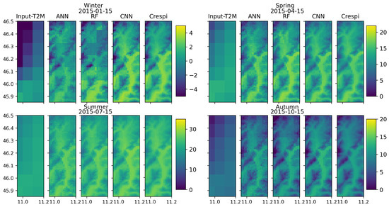
Figure 5.
Spatial plot of representative days for each season for input (ER5L-T2M), models (ANN, RF, and CNN), and target (Crespi T2M).
4.2. Average Metrics of Model Performance
Figure 6 shows the values of spatial-temporal aggregated metrics of the three models adopted (ANN, RF, and CNN) for downscaling across different seasons. The metrics are calculated for all 12 months; for example, for January, the metrics are computed for data across latitude (74), longitude (19), and 279 prediction days from 2010 to 2018. Then, the metrics are averaged for every season to compare and evaluate the performance of the models. CNN shows better values for metrics than others across all seasons, closely followed by RF. Particularly for summer and spring, both CNN and RF show values of metrics RMSE (1 °C, 1.2 °C), and R2 (0.94, 0.92) quite similar to each other, signifying close performance. However, particularly for winter, CNN performs better than RF, with the lowest RMSE (1.29 °C, 1.62 °C), MAE (1 °C, 1.26 °C), and the highest R2 (0.87, 0.79). This similar pattern of CNN performing better than RF is observed for autumn as well. On the other hand, the ANN model lags behind the RF and CNN models in terms of performance across all seasons, indicating its poor performance.
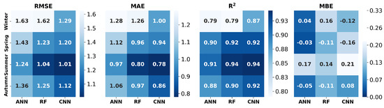
Figure 6.
Metrics heatmaps comparing the performance of the ANN, RF, and CNN models for winter, spring, summer, and autumn using RMSE, MAE, R2, and MBE over the test period from 2010–2018. The models with the best performance are shown with a darker blue color, whereas models with poor performance are shown in a lighter blue color.
All models exhibit seasonal variation in performance for downscaling spatial T2M. The best performance for all the models is obtained in summer, whereas the worst model performance is obtained in winter. The CNN model exhibits the best performance in summer (achieving RMSE = 1.01 °C, MAE = 0.78 °C, and R2 = 0.94), whereas the ANN model shows the lowest performance in winter (RMSE = 1.63 °C, MAE = 1.28 °C, and R2 = 0.79). The performances of the models for spring and autumn are very close to each other, which is better than winter and poorer than summer.
The aggregated MBE metric for all models shows lower biases, and its maximum value reaches only up to +0.21 °C and −0.16 °C (Figure 6). However, from the average metrics for MBE, it appears that the ANN model outperforms others, with the lowest MBE values across all seasons. To confirm this, we looked at the spatial distribution of MBE and its variation along the elevation for all models and seasons.
4.3. Spatial and Seasonal Variation in Model Performance
Figure 7 shows an elevation map of a study region (a), season-wise spatial distribution of MBE (b), and variation of MBE elevation bin-wise (c) for the ANN, RF, and CNN models. To show the spatial distribution, MBE is computed at each spatial location over the study region for the prediction time range of 2010 to 2018. The spatial distribution shows that the values of positive and negative MBE are much higher for ANN compared to its counterparts RF and CNN. The RF model shows comparable performance with CNN, although with higher values, both positive and negative, in particular in the winter. The analysis of MBE using spatial distributions reveals that the ANN model exhibits higher positive MBE at higher elevations and negative MBE at lower elevations, which results in compensating for MBE when aggregated over space and time, resulting in overall lower MBE metrics.
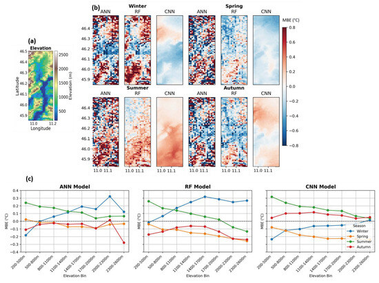
Figure 7.
Representation of MBE for the three proposed models. (a) Map of elevation for the study region. (b) Spatial distribution of MBE season-wise for ANN, RF, and CNN for testing period 2010–2018. (c) MBE elevation bin-wise for ANN, RF, and CNN for all seasons for testing period 2010–2018.
MBE varies with different elevations but also with seasons, showing clear patterns, particularly for summer and winter (Figure 7b,c). In summer, there is a decrease in positive MBE with an increase in elevation for all models, shown as a green line (Figure 7c). Conversely, for winter, there is an increase in positive MBE with an increase in elevation for models, except CNN, where MBE decreases with an increase in elevation, shown as a blue line (Figure 7c). In general, we observed that the ANN and RF models exhibit positive biases at higher elevations and negative biases at lower elevations. In addition, the seasonal pattern of MBE for elevation can be observed specifically for ANN and RF, whereas CNN shows a decrease in MBE for both summer and winter with an increase in elevation.
Figure 8c shows the variation of MAE with different elevations for each model for all seasons. MAE is also computed at each spatial location over a study region for the prediction time from 2010 to 2018. The ANN model shows an increase in MAE with increasing elevation across all seasons, with a slight decrease in MAE for elevation bins from 1700 m to 2300 m. However, the RF model shows different patterns, with relatively invariant MAE across elevations for almost all seasons except summer, where it decreases slightly with elevation.
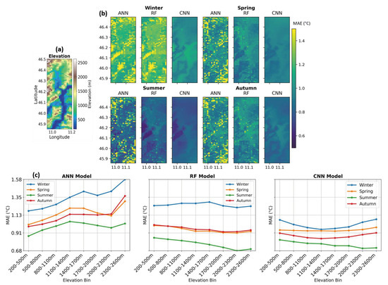
Figure 8.
Representation of MAE for the three proposed models. (a) Map of elevation for the study region. (b) Spatial distribution of MAE season-wise for ANN, RF, and CNN for testing period 2010–2018. (c) MAE elevation bin-wise for ANN, RF, and CNN for all seasons for testing period 2010–2018.
Conversely, for the CNN model, MAE decreases during summer with an increase in elevation, whereas in autumn, MAE remains consistent for all elevation bins. However, during winter, we observe mixed responses, with higher MAE values for both lower and higher elevation bins and lower MAE values for medium elevation bins for winter and autumn.
4.4. Sensitivity to Elevation
When we used ERA5L-T2M as the only predictor, both the ANN and RF models resulted in a scatter density plot exhibiting clearly visible horizontal lines (Figure 9). These patterns suggest that the relationship between predictor ERA5L-T2M and predictand is not well-captured, as also suggested by the lower correlation and R2 values. Conversely, when EL is provided as additional input along with ERA5L-T2M to the ANN and RF models, there is a significant improvement in model performance. The scatter plot no longer shows visible horizontal lines, suggesting a more consistent relationship between predictors and predictand. This improvement is marked by a notable increase in correlation coefficient and R2 values, as shown in Figure 9.

Figure 9.
Scatter plot between target T2M and model downscaled T2M for winter, considering predictor ERA5L-T2M alone (first row) and ERA5L-T2M with EL (second row).
When the CNN model is tested for only ERA5L-T2M as a predictor and with both ERA5L-T2M and EL as predictors, no noticeable difference in its performance is observed. Both cases resulted in identical correlation coefficients and R2 values. Furthermore, for CNN, data points on the scatter plot between observation and target lie more closely along the 1-to-1 line than for ANN and RF, indicating consistent model performance. The CNN showed a similar pattern of results across other seasons too, suggesting that the inclusion of elevation as an additional feature does not enhance model performance. This underscores the inherent capability of the CNN model in terms of extracting spatial information from the input datasets, making elevation an unnecessary additional input for the particular model even over complex terrain. However, for ANN and RF, the inclusion of elevation as an additional predictor plays a crucial role in enhancing the model’s performance in complex terrain.
4.5. Feature Importance of Models
Feature importance is a method used in ML to quantify the contribution of each input predictor or feature on model performance. Figure 10 shows the feature importance for the ANN, RF, and CNN models. In the study of downscaling spatial temperature, the identification of influential predictors is important for enhancing model accuracy and interpretability.
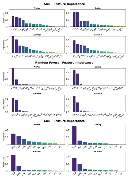
Figure 10.
Feature importance for ANN (first and second row), RF (third and fourth row), and CNN (fifth and sixth row) for all seasons.
During winter, for the ANN and RF models, a dominant feature is ERA5L-T2M, followed by EL, suggesting an emphasis on broader atmospheric conditions, followed by elevation. However, for the CNN model, for all the seasons, the dominant feature is T2M, followed by D2M, except in the winter, where D2M is the primary predictor, followed by ERA5L-T2M, indicating a different importance in the winter season. In spring, for the ANN and RF models, T2M still appears as a dominant feature, with EL as a secondary dominant feature. However, the importance given to ERA5L-T2M has been reduced, whereas there is an increase in importance given to EL. This adjustment suggests that there is a change in the relationship between temperature and elevation as the season transitions. In summer, ANN and RF see a consensus, with EL emerging as a dominant feature, followed by ERA5L-T2M, for both ANN and RF. This pattern underlines the key role of altitude on summer temperature, as expected. This might improve the relationship between temperature and altitude, potentially leading to the enhanced or better performance of the models in summer. In autumn, for ANN, EL is the dominant feature, followed by T2M, D2M, and SC. For RF, ERA5L-T2M emerges as a dominant feature once again, suggesting broader atmospheric conditions influencing daily mean temperature in autumn.
5. Discussion
Results suggest the superior performance of the CNN model in downscaling gridded daily mean T2M in complex terrain across all seasons, even with the aid of fewer features. This fact may be due to its ability to capture spatial features in datasets compared to other models. Additionally, CNN is inherently designed to handle image-like data and capture spatial dependencies in it, a feature that may be key to making it ideal for handling gridded datasets and well-suited for tasks such as spatial downscaling. In this study, the CNN model applies convolution filters to predictors (e.g., elevation, temperature) to detect gradients and spatial patterns. CNN captures temperature variations associated with elevation changes or other features by detecting edges and gradients in input data. During training time, these filters learn to represent these spatial relationships, allowing the model to identify how temperature is affected due to factors such as elevation or other features. The hierarchical architecture of CNN helps it capture low-level and high-level spatial features. For example, the first convolutional layer helps in capturing low-level spatial features like small changes in temperature, whereas deeper convolutional layers extract more complex relationships, e.g., the combined effect of wind and elevation on temperature. Thus, CNN builds a hierarchical presentation of data by stacking multiple layers, which allows it to recognize both broader and local spatial patterns in the dataset. Pooling layers reduces the dimension of feature maps by retaining most significant features. The final fully connected dense layers combine the captured spatial features and produce temperature predictions for each grid. This architecture of CNN enables it to effectively extract and learn complex spatial patterns, giving more accurate predictions for complex terrains.
Considering a downscaling ratio of 9, our study showed a good performance for CNN followed by RF for spatial downscaling of daily mean T2M. The metrics for CNN and RF show R2 > 0.90, RMSE < 1.25 °C, and MAE < 0.97 °C in all seasons except winter, where R2 ranges from 0.79 to 0.87, RMSE ranges from 1.29 °C to 1.63 °C, and MAE ranges from 1 °C to 1.28 °C. Moreover, ANN also shows comparable performance but lags behind CNN and RF in each season.
ANN and RF are predominantly employed for point scale downscaling [9,14,16]. Our study successfully tested these models for spatial downscaling of daily T2M. When compared to the Karaman and Akyurek [36] study that focused on downscaling monthly ERA5-Land T2M using RF for point scale downscaling, our study shows significant advantages in terms of temporal resolution with the RF model, with MAE values ranging from 0.80 °C to 1.26 °C and RMSE values from 1.04 °C to 1.62 °C across different seasons. Also, our results for daily downscaling of T2M using RF are comparable, with MAE (1.22 °C) and RMSE (1.65 °C) achieved on the monthly scale by Karaman and Akyurek [36]. Moreover, in our study, CNN attains the lowest MAE and RMSE among all models, with MAE from 0.78 °C to 1.00 °C and RMSE values ranging from 1.01 to 1.29, showing superior performance. Both studies show the robustness of ML models in downscaling T2M over complex topography. However, our focus on daily T2M provides finer temporal resolution with better performance for CNN.
Results indicate that ANN and RF also exhibit performances comparable to that of CNN, especially during spring and summer. Our study underlines and recommends the importance of considering elevation as an auxiliary predictor in enhancing the performance of ANN and RF in spatial downscaling of temperature in complex terrains. However, it also reveals no significant improvement for CNN, implying CNN’s ability to extract spatial features from input data without relying on elevation as an extra input feature. Notably, our study achieves a greater downscaling ratio (9) over complex terrains, advancing beyond the downscaling ratio in the earlier studies of 4 and 7, respectively [3,19].
We observed a pattern in seasonal variation in the models with better performance in summer and lower performance in winter, in line with earlier studies [36,59]. This strengthens the notion that seasonal variation significantly influences model performance. To analyze plausible reasons behind seasonal variation in the performance of the model, we conducted a seasonal comparison between input ERA5L-T2M and reference target T2M for errors. We calculated different metrics such as RMSE, MAE, and MBE between input ERA5L-T2M and target T2M data for different seasons (Figure 11).

Figure 11.
Error metrics RMSE, MAE, and MBE between ERA5L-T2M and reference target T2M (blue color bars) and of models with the reference target T2M (orange, green, and red color bars for ANN, RF, and CNN, respectively) for all seasons.
ERA5L-T2M exhibits the highest errors during winter, implying that ERA5L-T2M is less accurate in winter than in other seasons (Figure 11). Vanella et al. [60] observed similar results showing less accuracy of ERA5L-T2M data in winter and higher accuracy in autumn and summer when ERA5L-T2M is compared with ground-based observations over the regions of Lombardy, Apulia, Sicily, and Campania in Italy. This implies that large errors in input data during winter months may lead to poorer model performance. The errors reduced through spring and summer, reaching the lowest in autumn. However, it is also worth noting that, although the input seems most accurate in autumn, the best model performance was observed in summer and not in autumn. This suggests that errors in input data may be a contributing factor but not the sole reason for the lower performance of models in winter.
Some atmospheric processes are more frequent and exclusive to colder seasons, especially in winter, and are rarely present in other seasons. Examples include thermal inversions and katabatic winds, which occur at a very local scale. These types of phenomena are more common in winter because longer nights lead to a stronger radiation loss from the earth and, as a consequence, surface cooling. For instance, thermal inversions occur when the air near the surface is cooler than the air above [61]. Similarly, katabatic winds typically flow during the night, when air layers on mountain slopes cool faster than the valley atmosphere and make colder air drain toward valley floors, thus affecting the surface temperature there. The occurrence of such phenomena at the local scale recalls the complex interaction between topography and atmospheric conditions. While these processes are crucial in understanding temperature patterns, capturing them is still a significant challenge for numerical weather prediction models. These limitations may contribute to discrepancies in the performance of models during winter or colder seasons.
The MBE and MAE show distinct patterns across the models for their performance, particularly across elevation bins. For ANN and RF models, MBE increases with elevation in winter and decreases in summer. In winter, models seem to struggle more with elevation-related variations when ERA5L-T2M is the dominant feature. Additionally, complexities of winter conditions, such as snow cover and temperature inversions, introduce additional interactions that these models may not be able to take into full consideration. Conversely, during summer, MBE decreases along with the elevation when the dominant feature is the EL. This shift may result in a better understanding of the influence of elevation on temperature. The CNN models show a consistent decrease in MBE for both winter and summer across all elevations. The robustness of the CNN model and its superior performance can be attributed to the ability of the convolution layers to capture spatial patterns more effectively than ANN and RF.
The models also show variations of MAE along the elevation. The ANN model consistently shows the trend of increasing MAE towards higher elevations across all seasons, similar to findings [3] obtained for a study over the western United States on the downscaling temperature in complex terrains. It seems that ANN might struggle at higher elevations, with increasing complexity leading to higher MAE values irrespective of the seasons. The elevation distribution data have fewer data points at higher elevations (Figure 2), which could also play an important role in model training and performance. ANN with less exposure to high-elevation data points may not adequately learn specific patterns and conditions in these regions, which might have contributed to increased errors in those elevation ranges. However, the RF model shows comparatively stable MAE across elevation, with a slight decrease in summer. This stability implies that RF may manage to reduce errors more effectively as a result of the ensemble learning approach. On the other hand, the CNN model structure and its ability to extract spatial features from the data might mitigate the negative impacts of this data imbalance, giving lower and stable MBE and MAE across elevations. The observed errors in the MBE and MAE suggest that it would be important to consider shifts in feature importance, model structure, seasonal complexity, and data distribution in assessing model performance.
We observed variations in the performance of the ANN, RF, and CNN models depending on the inclusion of elevation as a predictor, as shown in Figure 9. The CNN model exhibited different behavior compared to the ANN and RF models, showing lower sensitivity to elevation as an explicit predictor. The possible reason behind these results can be attributed to differences in the architectures of CNN and other models. The CNN models are designed to handle images or grid data, making them effective at capturing spatial features and relationships between neighboring grid points. In the CNN model, convolutional layers apply filters to input data, which helps in detecting spatial features such as temperature gradients and features related to topography. Due to this, CNN can implicitly account for the effects of elevation through spatial data itself. For example, even when ERA5L-T2M was the only predictor, CNN can still understand the impact of elevation by learning from the spatial context, which includes temperature variations related to changes in elevations. The CNN model, indirectly through its convolution and pooling operations, has already learned elevation information. This ability of the CNN model to capture spatial dependencies explains why the explicit inclusion of elevation as an additional feature does not change its performance. On the other hand, the ANN and RF models do not have an inherent ability to capture spatial patterns and dependencies like CNN. For ANN and RF, the inclusion of elevation as an explicit predictor is crucial for improvement in their performance, especially in complex terrain. When ANN and RF provided ERA5L-T2M as the only predictor, excluding elevation, scatter density plots resulted in visible horizontal lines. The inclusion of elevation as an explicit predictor allows the ANN and RF models to capture the relationship between temperature and topography better, as shown by the disappearance of horizontal lines and improved R2 and correlation values.
Our results from the detailed feature importance analysis highlight distinct patterns in feature importance for the proposed models, showing their strengths and limitations under different seasons (Figure 10). The ANN model assigns significant importance to T2M and elevation, with moderate importance to all dynamic features across all seasons, except for static features (slope, aspect, and curvatures), which are consistently deemed less important. On the other hand, RF shows a very selective approach by selecting mostly ERA5L-T2M and EL as the primary predictors, with the others having less importance across all seasons. When we look at feature importance for CNN, it consistently has ERA5L-T2M as the dominant feature, followed by D2M across all seasons except winter, where D2M is the most dominant one. In addition to this, elevation has not been given importance at all, which suggests that the CNN model can extract spatial features on its own without a reliance on explicit input of elevation as additional features. This aspect of CNN underscores its characteristic strength in spatial feature extraction in the context of spatial temperature downscaling.
Based on our analysis, we found that the performance of models varied depending on the region and seasons, underscoring the importance of choosing the appropriate model for specific applications. The ANN model showed good performance for summer across the study region with moderate elevations. However, it struggled in regions with higher elevations, as shown by higher biases. Thus, the ANN model’s ability to capture nonlinear relationships between temperature and other predictors can be a good fit for regions with less complex terrains. The RF model showed better performance in handling both lower and higher elevations relatively well. The RF model exhibited consistent performance in summer, spring, and autumn, but its accuracy declined in winter, indicating its limited ability to capture extreme cold temperatures. On the other hand, the CNN model outperformed all others in the complex region across all seasons. Although its performance slightly declined in winter, with some further tuning, CNN could potentially also be used for predicting temperature for important practical applications such as frost forecasting.
6. Conclusions
ANN, RF, and CNN models were used for spatial downscaling daily mean temperature in the Non and Adige Valleys, a complex terrain in the Italian Alps. Results highlight that the CNN model exhibits superior performance across all seasons. RF performs closely with CNN, particularly in spring and summer, whereas ANN shows the lowest performance across all seasons. Our study achieved a greater downscaling ratio (9) over complex terrains compared to previous studies. Using elevation as an auxiliary predictor enhanced the performance of the ANN and RF models. Therefore, this study recommends using elevation as an auxiliary predictor in further studies for ANN and RF in complex terrains. However, we also observed no significant improvement when we added elevation as an auxiliary predictor for CNN, implying that it is not necessary for CNN. We observed that all ML models showed seasonal variation, with the best performance obtained in summer and the lowest in winter. Models show different patterns in variation of errors along elevation in other seasons. These findings are crucial, as they highlight how each model responds to differences in elevation and across seasons, providing insights into their strengths and limitations. This suggests that ANN and RF require additional adjustment for winters, whereas CNN stays constant without elevation data. This understanding of the variation of errors along elevation across different seasons is essential in future studies to enhance the performance of models in downscaling temperature in complex terrains.
While the proposed models exhibited strong performance in temperature variations, we acknowledge that one of the critical challenges in utilizing ML models in atmospheric research is their interpretability, as ML models are often considered black boxes. In this study, we addressed this challenge partially by doing a feature importance analysis to understand the contribution of different predictors to the performance of models. Although this analysis provides some insight into the various factors for model sensitivity, more is needed to ultimately bridge the gap between the predictive performance of the models and physical interpretation. Therefore, we recognize the need for future work to go deeper to understand the link between ML models and physical processes such as temperature and terrain features. In addition, efforts can be made to improve the performance of models in colder seasons, especially in winter, by including more features, such as vegetation indices and soil moisture. This is being addressed by ongoing research efforts under the international cooperative initiative TEAMx—Multi-scale transport and exchange processes in the atmosphere over mountains–programme and experiment. In line with that, we plan to work on the downscaling of seasonal temperature forecasts with a lead time of a few days over complex terrains, which may be helpful for applications such as frost forecasting.
Supplementary Materials
The following supporting information can be downloaded at: https://www.mdpi.com/article/10.3390/atmos15091085/s1, Table S1: CNN model performance for January with different predictor combinations with the metric table.
Author Contributions
S.B. developed the models, created plots, conducted analysis, structured the paper, and was responsible for writing an original draft of the manuscript and integrating feedback from coauthors. S.D.G. assisted in developing the model, analyzing the results, structuring the paper, and providing continuing guidance. M.V. assisted in the development of the model and provided essential technical support. D.Z. provided overall supervision of the work, helped analyze results, offered critical insight and feedback throughout the process, revised the manuscript throughout all of its versions, and was responsible for project initiation. L.T. assisted in deriving static features. M.P. was responsible for project initiation and provided useful guidance. M.M. contributed to reviewing the manuscript and providing suggestions and improvements. All authors have read and agreed to the published version of the manuscript.
Funding
The present research was partly funded by the European Union through the European Social Fund and by the Italian Ministry for the Universities and Research (MUR) through the National Operational Program (PON) “Ricerca e Innovazione 2014–2020, Dottorati di ricerca su tematiche dell’innovazione e green”. D.Z. acknowledges support from the Italian Ministry of University and Research under the project “DECIPHER—Disentangling mechanisms controlling atmospheric transport and mixing processes over mountain areas at different space- and timescales” funded by the European Union under NextGenerationEU, PRIN 2022, Prot. n. 2022NEWP4J.
Institutional Review Board Statement
Not applicable.
Informed Consent Statement
Not applicable.
Data Availability Statement
We developed ANN and CNN models using the TensorFlow deep learning library for building and training. We created an RF model leveraging the sci-kit learn package in Python. The ERA5-Land dataset is publicly available at https://cds.climate.copernicus.eu/cdsapp#!/dataset/reanalysis-era5-land, accessed on 20 February 2022. The reference target dataset is publicly available at https://doi.org/10.1594/PANGAEA.924502, accessed on 18 February 2022. The DEM dataset is available at https://dwtkns.com/srtm30m/, accessed on 1 March 2022.
Conflicts of Interest
The authors declare that they collaborated with the private company Amigo srl during this research. The authors declare no conflicts of interest.
Abbreviations
The abbreviations used in this manuscript are as follows:
| ANN | Artificial neural network |
| CNN | Convolutional neural network |
| C-curv | Cross-sectional curvature |
| D2M | Dew point temperature at 2 m AGL |
| DEM | Digital elevation model |
| ERA5L-T2M | ERA5-Land daily T2M |
| L-curv | Longitudinal curvature |
| MAE | Mean absolute error |
| R2 | Coefficient of determination |
| r | Pearson correlation coefficient |
| RF | Random forest |
| RMSE | Root mean square error |
| SC | Snow cover area fraction |
| SP | Surface pressure |
| SSHF | Surface sensible heat flux |
| SLHF | Surface latent heat flux |
| SNR | Surface net radiation |
| T2M | Temperature at 2 m AGL |
| U10 | Zonal wind at 10 m AGL |
| V10 | Meridional wind at 10 m AGL |
| WS | Wind speed |
References
- Kochkov, D.; Yuval, J.; Langmore, I.; Norgaard, P.; Smith, J.; Mooers, G.; Klöwer, M.; Lottes, J.; Rasp, S.; Düben, P.; et al. Neural general circulation models for weather and climate. Nature 2024, 632, 1060–1066. [Google Scholar] [CrossRef]
- Kleiber, W.; Katz, R.W.; Rajagopalan, B. Daily minimum and maximum temperature simulation over complex terrain. Ann. Appl. Stat. 2013, 7, 588–612. [Google Scholar] [CrossRef]
- Sha, Y.; Gagne, D.J., II; West, G.; Stull, R. Deep-learning-based gridded downscaling of surface meteorological variables in complex terrain. Part I: Daily maximum and minimum 2-m temperature. J. Appl. Meteorol. Climatol. 2020, 59, 2057–2073. [Google Scholar] [CrossRef]
- Lin, J.; Wei, K.; Guan, Z. Exploring the connection between morphological characteristic of built-up areas and surface heat islands based on MSPA. Urban Clim. 2024, 53, 101764. [Google Scholar] [CrossRef]
- Zheng, Y.; Han, Q.; Keeffe, G. An evaluation of different landscape design scenarios to improve outdoor thermal comfort in Shenzhen. Land 2024, 13, 65. [Google Scholar] [CrossRef]
- Lo, J.C.F.; Yang, Z.L.; Pielke, R.A., Sr. Assessment of three dynamical climate downscaling methods using the Weather Research and Forecasting (WRF) model. J. Geophys. Res. Atmos. 2008, 113, D09112. [Google Scholar] [CrossRef]
- Wang, X.; Tolksdorf, V.; Otto, M.; Scherer, D. WRF-based dynamical downscaling of ERA5 reanalysis data for High Mountain Asia: Towards a new version of the High Asia Refined analysis. Int. J. Climatol. 2021, 41, 743–762. [Google Scholar] [CrossRef]
- Liu, G.; Zhang, R.; Hang, R.; Ge, L.; Shi, C.; Liu, Q. Statistical downscaling of temperature distributions in southwest China by using terrain-guided attention network. IEEE J. Sel. Top. Appl. Earth Obs. Remote Sens. 2023, 16, 1678–1690. [Google Scholar] [CrossRef]
- Pang, B.; Yue, J.; Zhao, G.; Xu, Z. Statistical downscaling of temperature with the random forest model. Adv. Meteorol. 2017, 2017, 7265178. [Google Scholar] [CrossRef]
- Azari, B.; Hassan, K.; Pierce, J.; Ebrahimi, S. Evaluation of machine learning methods application in temperature prediction. Environ. Eng. 2022, 8, 1–12. [Google Scholar] [CrossRef]
- Kuhn, M.; Olefs, M. Elevation-Dependent Climate Change in the European Alps. In Oxford Research Encyclopedia of Climate Science; Oxford University Press: Oxford, UK, 2020. [Google Scholar] [CrossRef]
- Goyal, M.K.; Ojha, C. Downscaling of surface temperature for lake catchment in an arid region in India using linear multiple regression and neural networks. Int. J. Climatol. 2012, 32, 552–566. [Google Scholar] [CrossRef]
- Anandhi, A.; Srinivas, V.; Kumar, D.N.; Nanjundiah, R.S. Role of predictors in downscaling surface temperature to river basin in India for IPCC SRES scenarios using support vector machine. Int. J. Climatol. J. R. Meteorol. Soc. 2009, 29, 583–603. [Google Scholar] [CrossRef]
- Duhan, D.; Pandey, A. Statistical downscaling of temperature using three techniques in the Tons River basin in Central India. Theor. Appl. Climatol. 2015, 121, 605–622. [Google Scholar] [CrossRef]
- Mouatadid, S.; Easterbrook, S.; Erler, A.R. A machine learning approach to non-uniform spatial downscaling of climate variables. In Proceedings of the 2017 IEEE international conference on data mining workshops (ICDMW), New Orleans, LA, USA, 18–21 November 2017; pp. 332–341. [Google Scholar] [CrossRef]
- Nourani, V.; Razzaghzadeh, Z.; Baghanam, A.H.; Molajou, A. ANN-based statistical downscaling of climatic parameters using decision tree predictor screening method. Theor. Appl. Climatol. 2019, 137, 1729–1746. [Google Scholar] [CrossRef]
- Hanoon, M.S.; Ahmed, A.N.; Zaini, N.; Razzaq, A.; Kumar, P.; Sherif, M.; Sefelnasr, A.; El-Shafie, A. Developing machine learning algorithms for meteorological temperature and humidity forecasting at Terengganu state in Malaysia. Sci. Rep. 2021, 11, 18935. [Google Scholar] [CrossRef]
- Hutengs, C.; Vohland, M. Downscaling land surface temperatures at regional scales with random forest regression. Remote Sens. Environ. 2016, 178, 127–141. [Google Scholar] [CrossRef]
- Baño-Medina, J.; Manzanas, R.; Gutiérrez, J.M. Configuration and intercomparison of deep learning neural models for statistical downscaling. Geosci. Model Dev. 2020, 13, 2109–2124. [Google Scholar] [CrossRef]
- Barry, R.G. Mountain Weather and Climate; Cambridge University Press: Cambridge, UK, 2008. [Google Scholar]
- Serafin, S.; Zardi, D. Daytime Development of the Boundary Layer over a Plain and in a Valley under Fair Weather Conditions: A Comparison by Means of Idealized Numerical Simulations. J. Atmos. Sci. 2011, 68, 2128–2141. [Google Scholar] [CrossRef]
- Geiger, R.; Aron, R.H.; Todhunter, P. The Climate Near the Ground; Vieweg+Teubner Verlag: Wiesbaden, Germany, 1995; pp. XVI,528. [Google Scholar] [CrossRef]
- Whiteman, C.D. Mountain Meteorology: Fundamentals and Applications; Oxford University Press: Oxford, UK, 2000. [Google Scholar]
- Grigiante, M.; Mottes, F.; Zardi, D.; de Franceschi, M. Experimental solar radiation measurements and their effectiveness in setting up a real-sky irradiance model. Renew. Energy 2011, 36, 1–8. [Google Scholar] [CrossRef]
- Castelli, M.; Stöckli, R.; Zardi, D.; Tetzlaff, A.; Wagner, J.; Belluardo, G.; Zebisch, M.; Petitta, M. The HelioMont method for assessing solar irradiance over complex terrain: Validation and improvements. Remote Sens. Environ. 2014, 152, 603–613. [Google Scholar] [CrossRef]
- Farina, S.; Marchio, M.; Barbano, F.; di Sabatino, S.; Zardi, D. Characterization of the Morning Transition over the Gentle Slope of a Semi-Isolated Massif. J. Appl. Meteorol. Climatol. 2023, 62, 449–466. [Google Scholar] [CrossRef]
- Conangla, L.; Cuxart, J.; Jiménez, M.A.; Martínez-Villagrasa, D.; Ramon Miro, J.; Tabarelli, D.; Zardi, D. Cold-air pool evolution in a wide Pyrenean valley. Int. J. Climatol. 2018, 38, 2852–2865. [Google Scholar] [CrossRef]
- Farina, S.; Zardi, D. Understanding Thermally Driven Slope Winds: Recent Advances and Open Questions. Bound.-Layer Meteorol. 2023, 189, 5–52. [Google Scholar] [CrossRef]
- De Wekker, S.F.J.; Kossmann, M.; Knievel, J.C.; Giovannini, L.; Gutmann, E.D.; Zardi, D. Meteorological Applications Benefiting from an Improved Understanding of Atmospheric Exchange Processes over Mountains. Atmosphere 2018, 9, 371. [Google Scholar] [CrossRef]
- Tomasi, E.; Giovannini, L.; Falocchi, M.; Antonacci, G.; Jiménez, P.A.; Kosovic, B.; Alessandrini, S.; Zardi, D.; Delle Monache, L.; Ferrero, E. Turbulence parameterizations for dispersion in sub-kilometer horizontally non-homogeneous flows. Atmos. Res. 2019, 228, 122–136. [Google Scholar] [CrossRef]
- Giovannini, L.; Ferrero, E.; Karl, T.; Rotach, M.W.; Staquet, C.; Trini Castelli, S.; Zardi, D. Atmospheric Pollutant Dispersion over Complex Terrain: Challenges and Needs for Improving Air Quality Measurements and Modeling. Atmosphere 2020, 11, 646. [Google Scholar] [CrossRef]
- Chow, F.K.; Schär, C.; Ban, N.; Lundquist, K.A.; Schlemmer, L.; Shi, X. Crossing multiple gray zones in the transition from mesoscale to microscale simulation over complex terrain. Atmosphere 2019, 10, 274. [Google Scholar] [CrossRef]
- Mutiibwa, D.; Strachan, S.; Albright, T. Land surface temperature and surface air temperature in complex terrain. IEEE J. Sel. Top. Appl. Earth Obs. Remote Sens. 2015, 8, 4762–4774. [Google Scholar] [CrossRef]
- Li, W.; Ni, L.; Li, Z.l.; Duan, S.B.; Wu, H. Evaluation of machine learning algorithms in spatial downscaling of MODIS land surface temperature. IEEE J. Sel. Top. Appl. Earth Obs. Remote Sens. 2019, 12, 2299–2307. [Google Scholar] [CrossRef]
- Wang, F.; Tian, D.; Lowe, L.; Kalin, L.; Lehrter, J. Deep learning for daily precipitation and temperature downscaling. Water Resour. Res. 2021, 57, e2020WR029308. [Google Scholar] [CrossRef]
- Karaman, Ç.H.; Akyürek, Z. Evaluation of near-surface air temperature reanalysis datasets and downscaling with machine learning based Random Forest method for complex terrain of Turkey. Adv. Space Res. 2023, 71, 5256–5281. [Google Scholar] [CrossRef]
- Sebbar, B.e.; Khabba, S.; Merlin, O.; Simonneaux, V.; Hachimi, C.E.; Kharrou, M.H.; Chehbouni, A. Machine-learning-based downscaling of hourly ERA5-Land air temperature over mountainous regions. Atmosphere 2023, 14, 610. [Google Scholar] [CrossRef]
- Crespi, A.; Matiu, M.; Bertoldi, G.; Petitta, M.; Zebisch, M. A high-resolution gridded dataset of daily temperature and precipitation records (1980–2018) for Trentino-South Tyrol (north-eastern Italian Alps). Earth Syst. Sci. Data 2021, 13, 2801–2818. [Google Scholar] [CrossRef]
- Panziera, L.; Giovannini, L.; Laiti, L.; Zardi, D. The relation between circulation types and regional Alpine climate. Part I: Synoptic climatology of Trentino. Int. J. Climatol. 2015, 35, 4655–4672. [Google Scholar] [CrossRef]
- Panziera, L.; Giovannini, L.; Laiti, L.; Zardi, D. The relation between circulation types and regional Alpine climate. Part II: The dependence of the predictive skill on the vertical level of the classification for Trentino. Int. J. Climatol. 2016, 36, 2189–2199. [Google Scholar] [CrossRef]
- De Ros, G.; Anfora, G.; Grassi, A.; Ioriatti, C. The potential economic impact of Drosophila suzukii on small fruits production in Trentino (Italy). IOBC-WPRS Bull 2013, 91, 317–321. [Google Scholar]
- Risso, W.A.; Barquet, A.; Brida, J.G. Causality between economic growth and tourism expansion: Empirical evidence from Trentino-Alto Adige. Tour. Int. Multidiscip. J. Tour. 2010, 5, 87–98. [Google Scholar]
- Laiti, L.; Zardi, D.; de Franceschi, M.; Rampanelli, G.; Giovannini, L. Analysis of the diurnal development of a lake-valley circulation in the Alps based on airborne and surface measurements. Atmos. Chem. Phys. 2014, 14, 9771–9786. [Google Scholar] [CrossRef]
- Giovannini, L.; Laiti, L.; Zardi, D.; de Franceschi, M. Climatological characteristics of the Ora del Garda wind in the Alps. Int. J. Climatol. 2015, 35, 4103–4115. [Google Scholar] [CrossRef]
- Giovannini, L.; Laiti, L.; Serafin, S.; Zardi, D. The thermally driven diurnal wind system of the Adige Valley in the Italian Alps. Q. J. R. Meteorol. Soc. 2017, 143, 2389–2402. [Google Scholar] [CrossRef]
- Lezama Valdes, L.M.; Katurji, M.; Meyer, H. A machine learning based downscaling approach to produce high spatio-temporal resolution land surface temperature of the antarctic dry valleys from MODIS data. Remote Sens. 2021, 13, 4673. [Google Scholar] [CrossRef]
- Xu, S.; Zhao, Q.; Yin, K.; He, G.; Zhang, Z.; Wang, G.; Wen, M.; Zhang, N. Spatial downscaling of land surface temperature based on a multi-factor geographically weighted machine learning model. Remote Sens. 2021, 13, 1186. [Google Scholar] [CrossRef]
- Ehsani, A.H.; Quiel, F. Geomorphometric feature analysis using morphometric parameterization and artificial neural networks. Geomorphology 2008, 99, 1–12. [Google Scholar] [CrossRef]
- Ding, S.; Zhi, X.; Lyu, Y.; Ji, Y.; Guo, W. Deep Learning for Daily 2-m Temperature Downscaling. Earth Space Sci. 2024, 11, e2023EA003227. [Google Scholar] [CrossRef]
- Acharya, N.; Chattopadhyay, S.; Mohanty, U.; Dash, S.; Sahoo, L. On the bias correction of general circulation model output for Indian summer monsoon. Meteorol. Appl. 2013, 20, 349–356. [Google Scholar] [CrossRef]
- Martin, T.C.; Rocha, H.R.; Perez, G.M. Fine scale surface climate in complex terrain using machine learning. Int. J. Climatol. 2021, 41, 233–250. [Google Scholar] [CrossRef]
- Shrivastava, V.K.; Shrivastava, A.; Sharma, N.; Mohanty, S.N.; Pattanaik, C.R. Deep learning model for temperature prediction: An empirical study. Model. Earth Syst. Environ. 2023, 9, 2067–2080. [Google Scholar] [CrossRef]
- Ghafarian, F.; Wieland, R.; Lüttschwager, D.; Nendel, C. Application of extreme gradient boosting and Shapley Additive explanations to predict temperature regimes inside forests from standard open-field meteorological data. Environ. Model. Softw. 2022, 156, 105466. [Google Scholar] [CrossRef]
- Wang, Y.V.; Kim, S.H.; Lyu, G.; Lee, C.L.; Lee, G.; Min, K.H.; Kafatos, M.C. Relative importance of radar variables for nowcasting heavy rainfall: A machine learning approach. IEEE Trans. Geosci. Remote Sens. 2022, 61, 4100314. [Google Scholar] [CrossRef]
- Breiman, L. Random forests. Mach. Learn. 2001, 45, 5–32. [Google Scholar] [CrossRef]
- Aloysius, N.; Geetha, M. A review on deep convolutional neural networks. In Proceedings of the 2017 International Conference on Communication and Signal Processing (ICCSP), Chennai, India, 6–8 April 2017; pp. 588–592. [Google Scholar] [CrossRef]
- Gu, J.; Wang, Z.; Kuen, J.; Ma, L.; Shahroudy, A.; Shuai, B.; Liu, T.; Wang, X.; Wang, G.; Cai, J.; et al. Recent advances in convolutional neural networks. Pattern Recognit. 2018, 77, 354–377. [Google Scholar] [CrossRef]
- Tolias, G.; Sicre, R.; Jégou, H. Particular object retrieval with integral max-pooling of CNN activations. arXiv 2015, arXiv:1511.05879. [Google Scholar] [CrossRef]
- Li, Y.; Yan, X. Statistical downscaling of monthly mean temperature for Kazakhstan in Central Asia. Clim. Res. 2017, 72, 101–110. [Google Scholar] [CrossRef]
- Vanella, D.; Longo-Minnolo, G.; Belfiore, O.R.; Ramírez-Cuesta, J.M.; Pappalardo, S.; Consoli, S.; D’Urso, G.; Chirico, G.B.; Coppola, A.; Comegna, A.; et al. Comparing the use of ERA5 reanalysis dataset and ground-based agrometeorological data under different climates and topography in Italy. J. Hydrol. Reg. Stud. 2022, 42, 101182. [Google Scholar] [CrossRef]
- Czarnecka, M.; Nidzgorska-Lencewicz, J.; Rawicki, K. Thermal inversions and sulphure dioxide concentrations in some Polish cities in the winter season. J. Elem. 2016, 21, 1001–1015. [Google Scholar] [CrossRef]
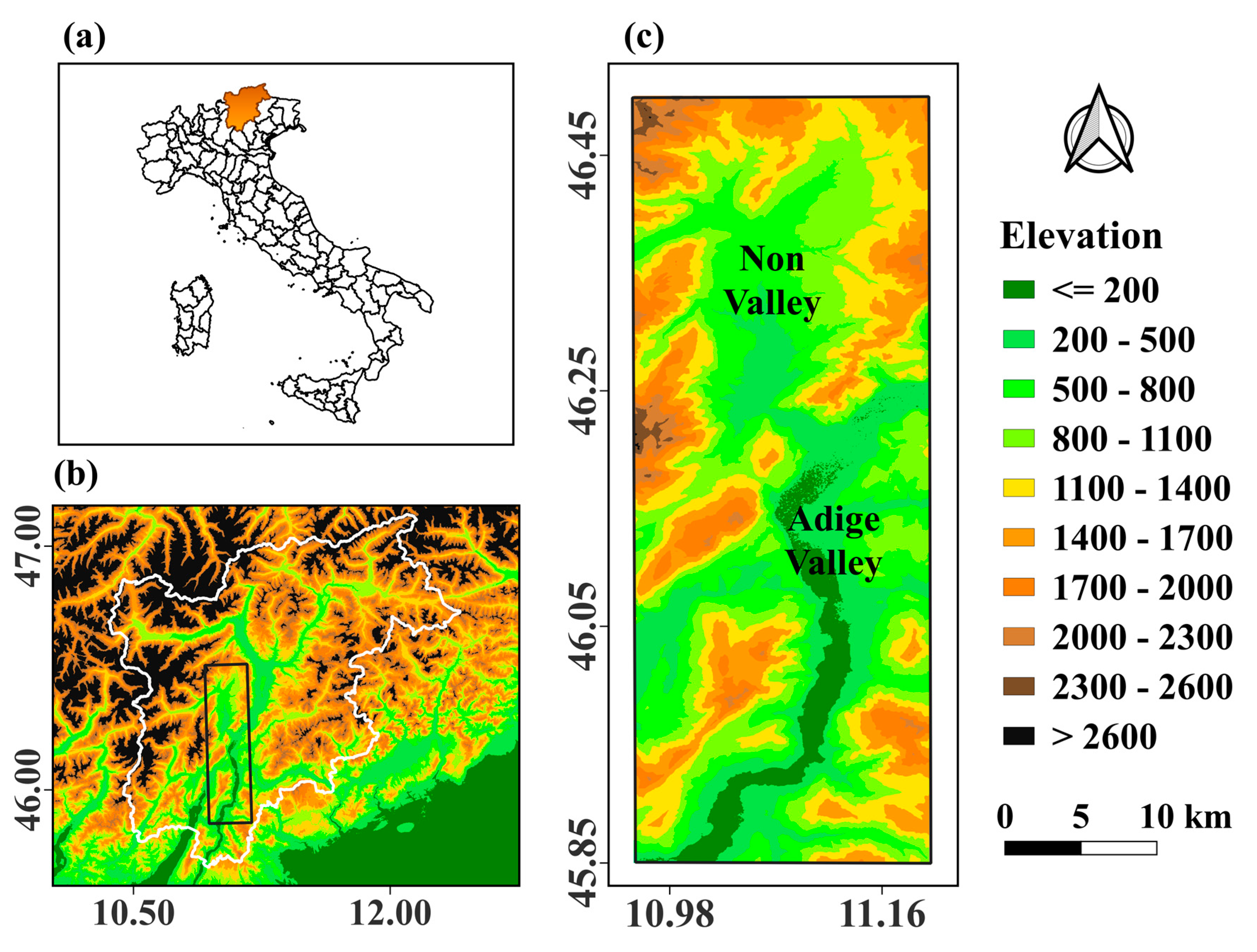
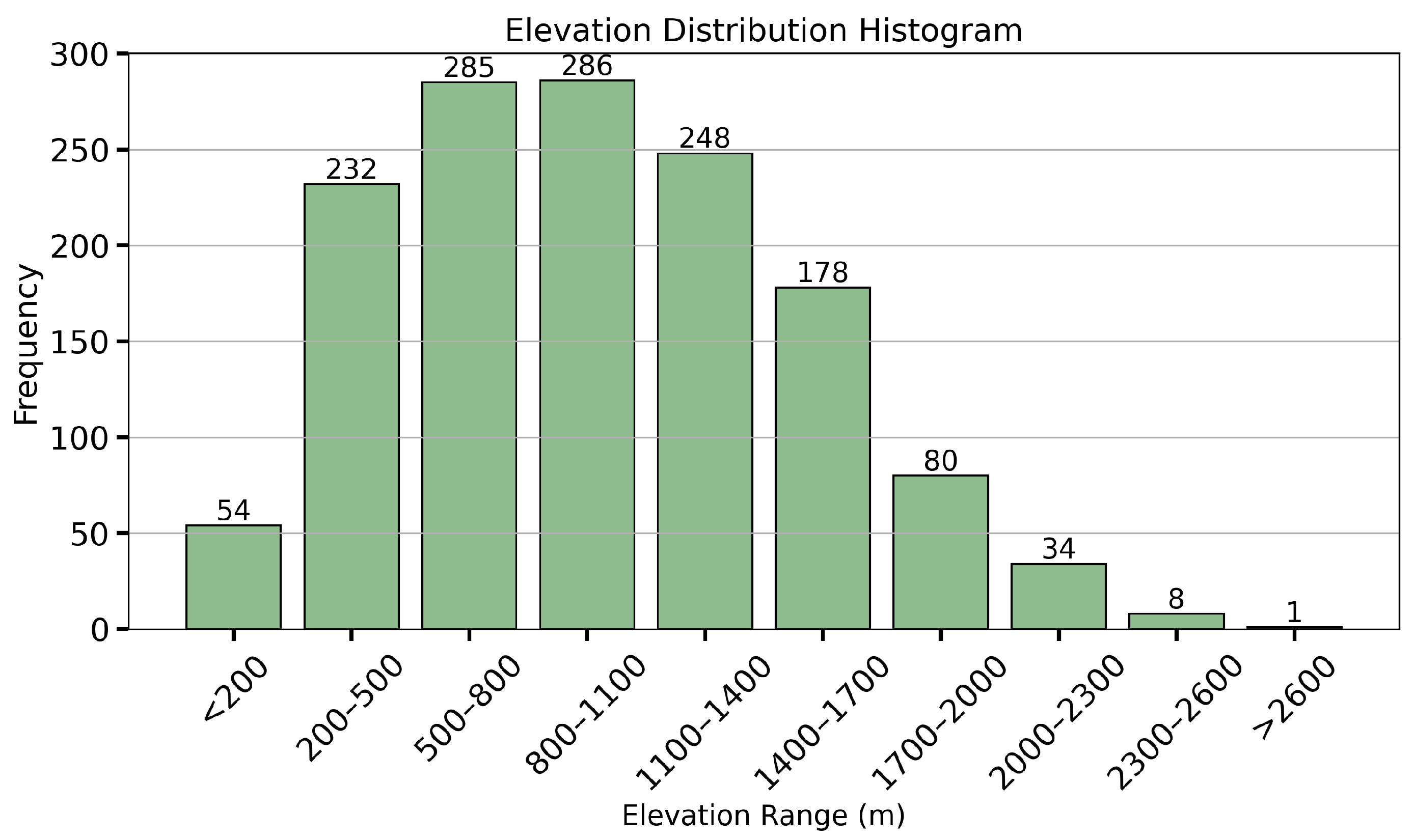
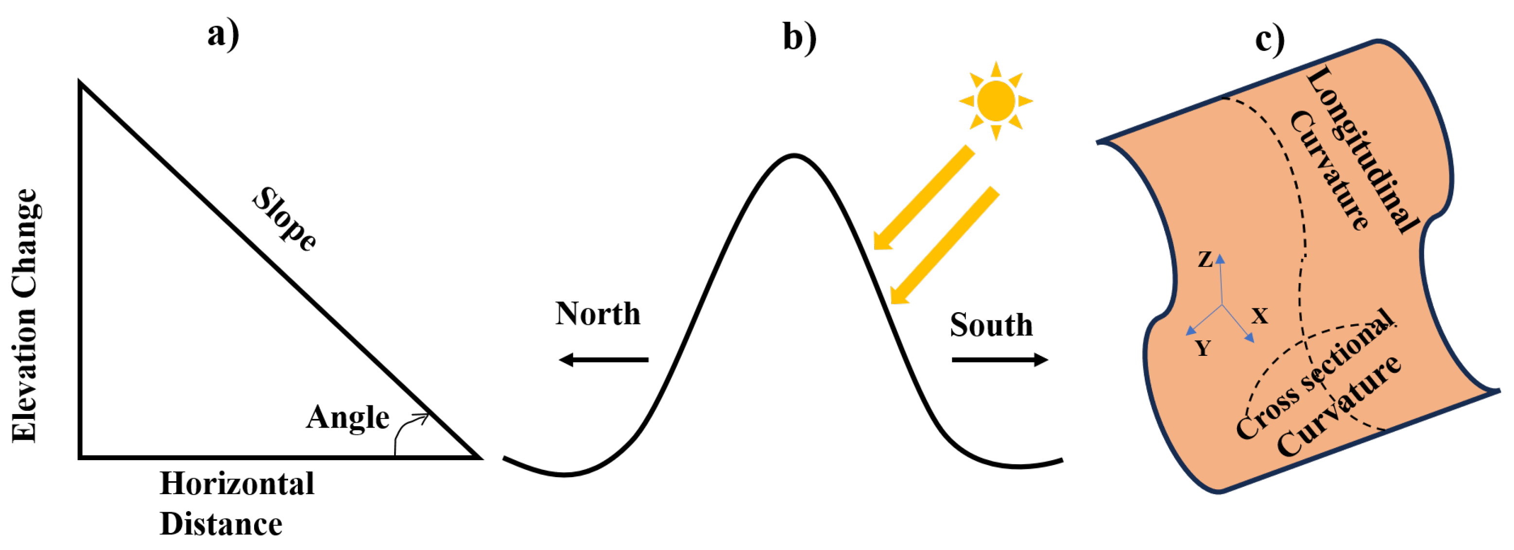
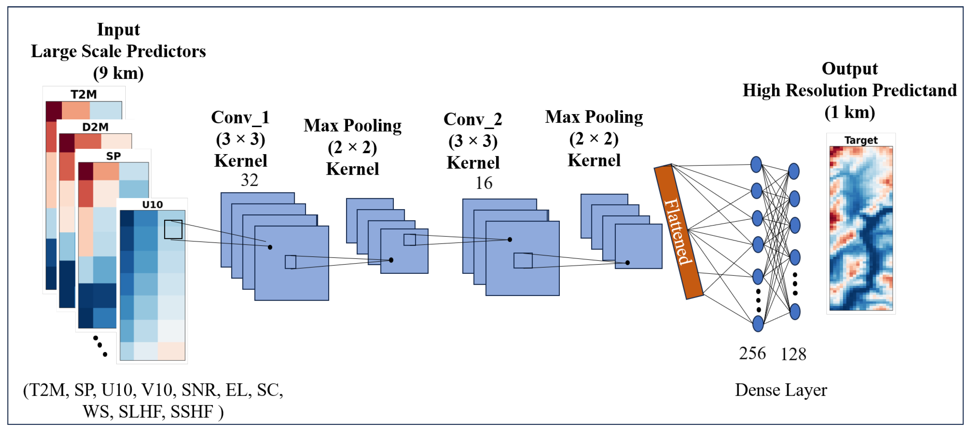
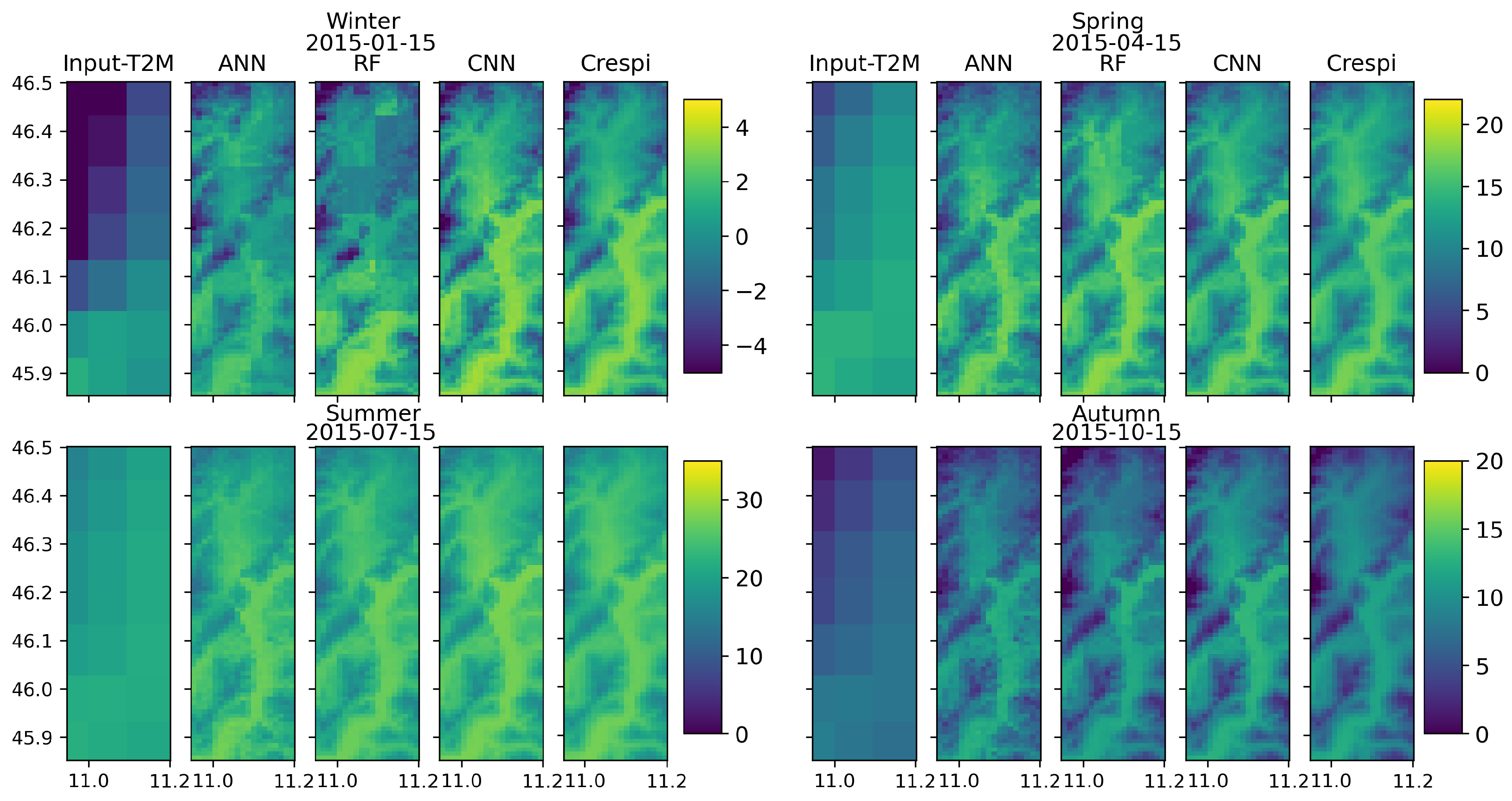
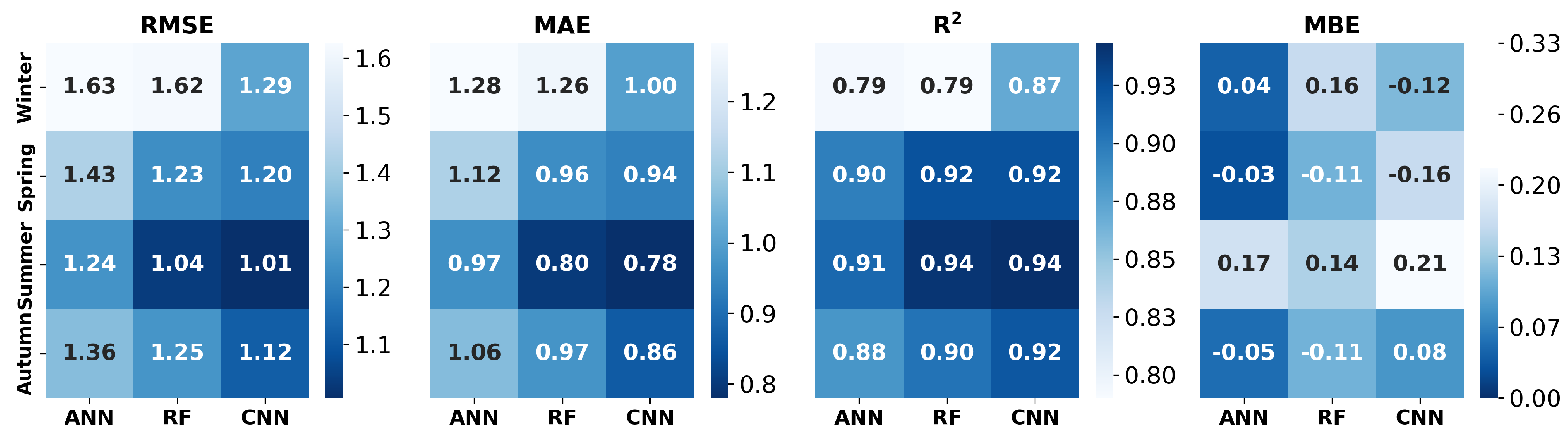
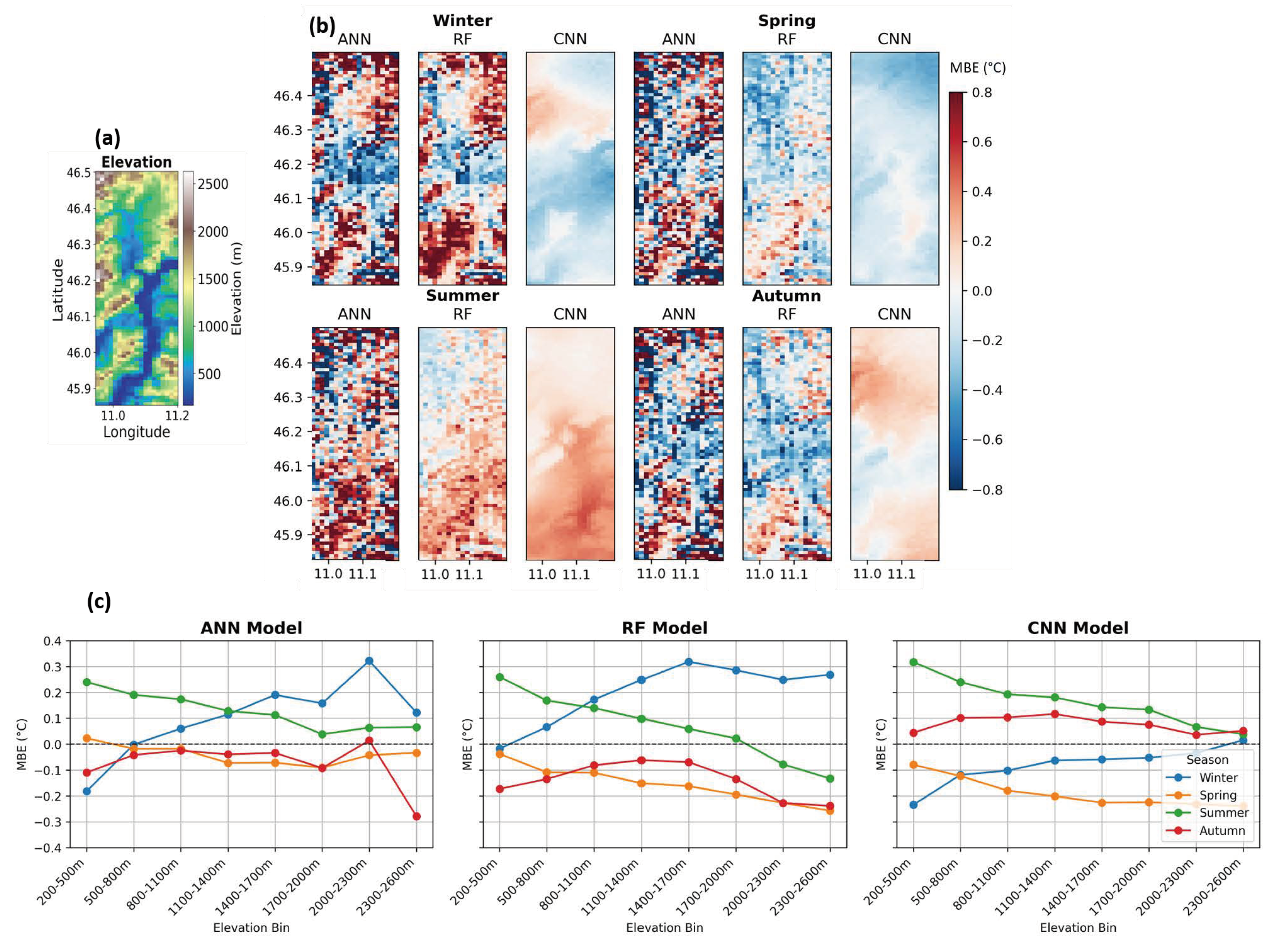

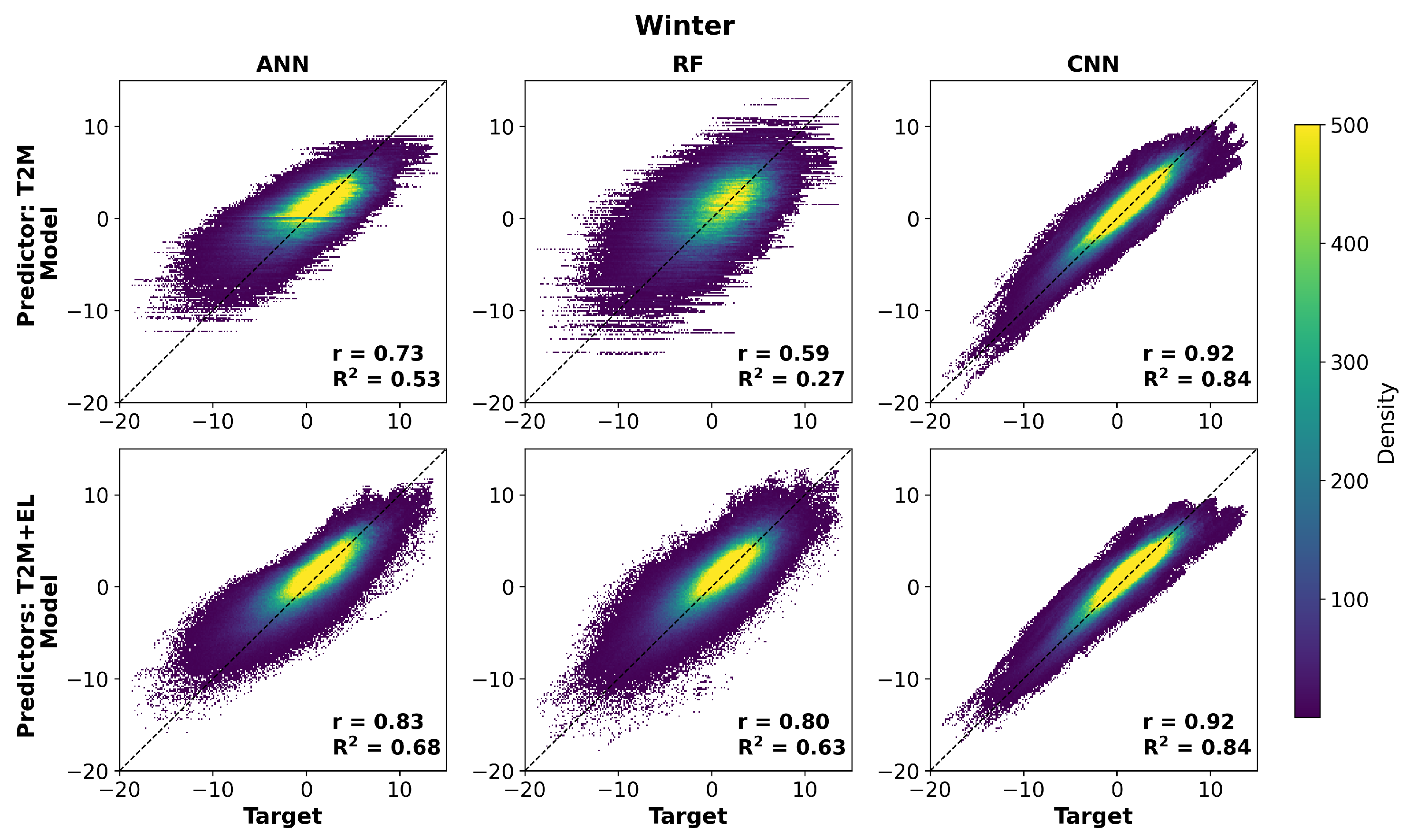
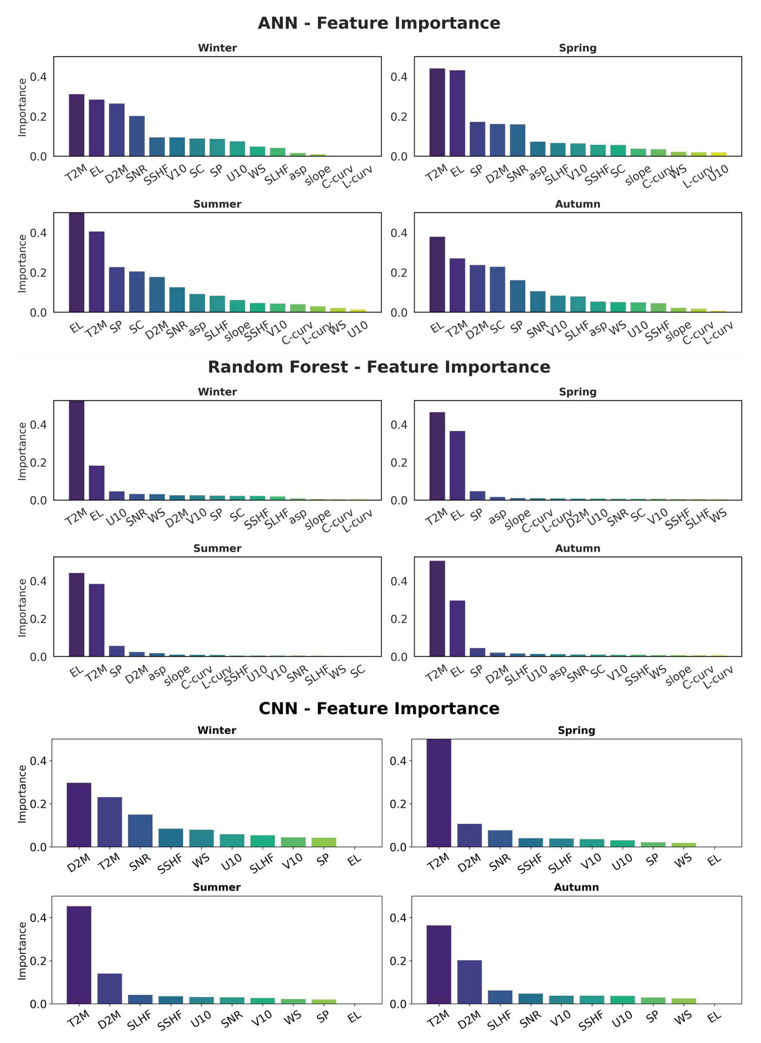
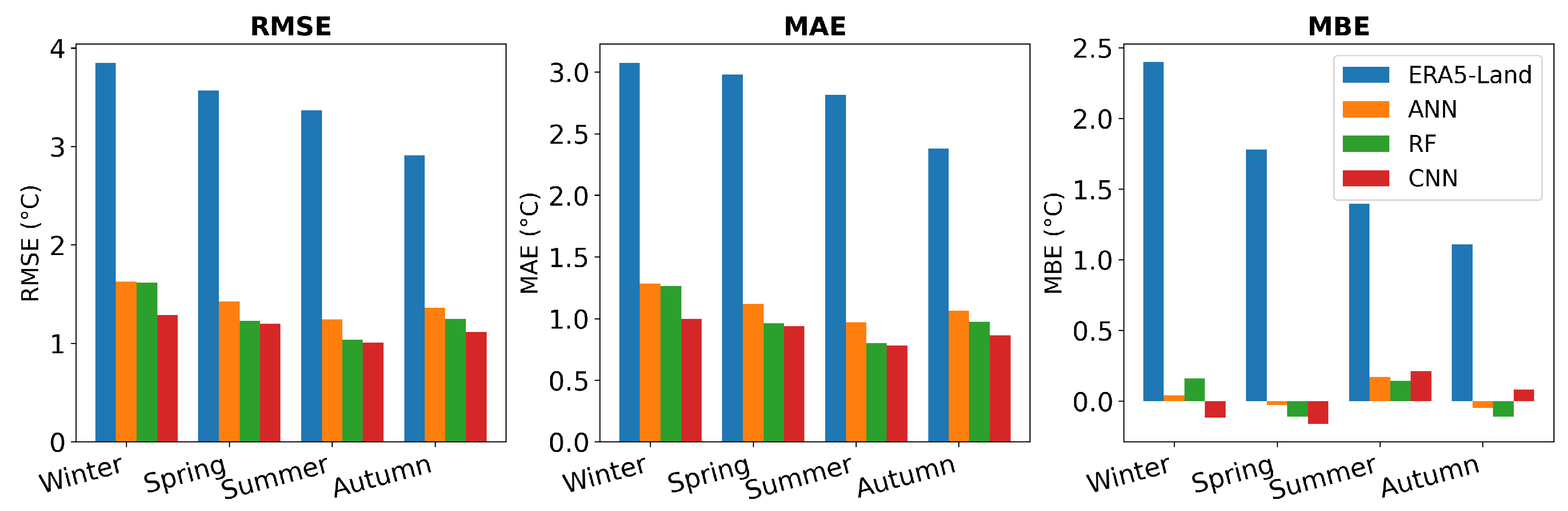
Disclaimer/Publisher’s Note: The statements, opinions and data contained in all publications are solely those of the individual author(s) and contributor(s) and not of MDPI and/or the editor(s). MDPI and/or the editor(s) disclaim responsibility for any injury to people or property resulting from any ideas, methods, instructions or products referred to in the content. |
© 2024 by the authors. Licensee MDPI, Basel, Switzerland. This article is an open access article distributed under the terms and conditions of the Creative Commons Attribution (CC BY) license (https://creativecommons.org/licenses/by/4.0/).