Future Scenarios of Design Rainfall Due to Upcoming Climate Changes in NSW, Australia

Abstract

The occurrence of rainfall is significantly affected by climate change around the world. While in some places this is likely to result in increases in rainfall, both winter and summer rainfall in most parts of New South Wales (NSW), Australia are projected to decrease considerably due to climate change. This has the potential to impact on a range of hydraulic and hydrologic design considerations for water engineers, such as the design and construction of stormwater management systems. These systems are currently planned based on past extreme rain event data, and changes in extreme rainfall amounts due to climate change could lead to systems being seriously undersized (if extreme precipitation events become more common and/or higher in magnitude) or oversized (if extreme rainfall events become less frequent or decrease in magnitude). Both outcomes would have potentially serious consequences. Consequently, safe, efficient, and cost-effective urban drainage system design requires the consideration of impacts arising from climate change on the approximation of design rainfall. This study examines the impacts of climate change on the probability of occurrence of daily extreme rainfall in New South Wales (NSW), Australia. The analysis was performed for 29 selected meteorological stations located across NSW. Future design rainfall in this research was determined from the projected rainfall for different time periods (2020 to 2039, 2040 to 2059, 2060 to 2079, and 2080 to 2099). The results of this study show that design rainfall for the standard return periods was, in most cases, lower than that derived employing the design rainfall obtained from the Australian Bureau of Meteorology (BoM). While most of the analysed meteorological stations showed significantly different outcomes using the climate change scenario data, this varied considerably between stations and different time periods. This suggests that more work needs to be performed at the local scale to incorporate climate change predicted rainfall data into future stormwater system designs to ensure the best outcomes.

1. Introduction

Design rainfall, which is the most essential component for the design of stormwater management infrastructure, is represented using an intensity–frequency–duration (IFD) chart/table. The IFD curve or chart is the probabilistic representation of a rainfall event occurring over a specific period of recurrence interval. This is critically important as engineers use design rainfall to estimate the required capacities of nearly all stormwater infrastructure types, from small-scale installations like gutters and roofs to large-scale infrastructure like basins and dams. The correct sizing of this infrastructure has considerable implications for flood mitigation and safety as well as the efficient use of resources with over-designed systems being unnecessarily expensive and under-designed systems potentially leading to loss of life and property.

For the determination of design rainfall, the IFD table/chart is traditionally developed by analysing the frequency of extreme rainfall from historical data sets. While this approach has generally served well in the past, the speed and anticipated magnitude of future climate-driven changes in rainfall suggest that it may no longer be appropriate [1]. This is because climate change is and will continue to impact the connection between extreme rainfall intensity, frequency, and duration over time. As such, continuing to use historical rainfall data to design stormwater management systems will likely result in systems that are either considerably under- or over-designed for future conditions [2,3,4,5].

The potential sensitivity of design rainfall to a changing climate has been widely recognised by many researchers around the world [6,7,8,9,10]. For example, Yilmaz and Perera [10] discovered the need to determine future design rainfall from future climate data. They developed non-stationary GEV models to investigate the potential influences of climate change on extreme rainfall and found no advantages over stationary GEV models in Melbourne, Australia. Consequently, Yilmaz et al. [9] determined the role of IPO in estimating the design rainfall in Victoria, Australia, and found higher rainfall intensities for a long duration. However, the studies of Yilmaz and Perera [10] and Yilmaz et al. [9] were based on only one meteorological station in Melbourne, Australia. Nevertheless, they emphasized the requirements for spatial analysis of extreme rainfall data from multiple observation stations. Furthermore, climate change impacts on the rainfall temporal patterns were not considered by Yilmaz and Perera [10] and Yilmaz et al. [9]. However, it is one of the critical aspects to be considered for future stormwater management infrastructure design. Therefore, Hettiarachchi et al. [7] evaluated the influence of climate change on the temporal patterns of rainfall events in Minnesota, United States. They observed that the projected temporal patterns have the potential to increase flood risks by up to 170%. Again, their study investigated only one rain gauge station, and extrapolation for large spatial scales without further analysis is discouraged.

Consequently, the ambiguity in the determination of design rainfall in varied climates due to changes in long-term weather patterns was investigated in West Yorkshire, England by Fadhel et al. [6]. Their study discovered that the variability in the proportion of design rainfall change varies significantly depending on the reference period of the bias correction. Traditionally, bias correction on climatic model outputs is applied to account for errors for the improvement of fitting and observations. Further analysis was conducted on the spatial variability of extreme precipitation from individual meteorological stations as well as from gridded data from Australia, Japan, Europe, and the USA by Myhre et al. [8]. Their study discovered that extreme precipitation events will be doubled for each degree of temperature increase. As a result, it is anticipated there will be more natural disasters, e.g., intensified floods, erosion of soil, landslides, and health impacts from impacts of climate change [9,11]. Consequently, a better understanding of climate change influence on design rainfall is essential for the derivation of design rainfall.

Traditionally, design rainfall is determined for several recurrence intervals from historical rainfall without considering climate change impacts [10]. This assumption has the potential to either over- or underestimate future design rainfall due to the impacts of changing climate from anthropogenic sources [12]. When design rainfall is underestimated, storm drainage infrastructures can be inadequate, leading to flooding in areas thought protected, which has been observed by many researchers [13,14]. Consequently, infrastructure, property, and the environment in urban areas are at risk of flooding from the changing rainfall pattern [15]. This outcome is further supported by an analysis of the recent trend in Australian rainfall [16].

Although many researchers accepted the impacts of climate change on design rainfall derivation, their influences are considered in the national guidelines in many countries around the world. In Australia, stormwater management infrastructures are designed using the design rainfall obtained from the Australian Bureau of Meteorology (BoM), which is the national guideline in Australia. However, the impacts of climate change have not been reflected by BoM [17]. As a result, currently designed stormwater management infrastructures accept the uncertainty to combat in the changing climate. From the motivation of a better understanding of the climate change impacts on the probability of occurrence of extreme rainfall in NSW, Australia, this study investigates the deviation of daily design rainfall due to climate change. The primary focus was to estimate the design rainfall using the projected data and to assess the current Australian standard. This research emphasises the importance of the amalgamation of climate change impacts on design rainfall in Australia. The study uses a large number of stations and time frames to identify the spatial and temporal impacts of potential climate change and show these are large enough to invalidate our current approach. Current knowledge on climate change influence on extreme rainfall will be further strengthened by the outcomes of this research. The study has the potential to understand the possible uncertainty in the stormwater management infrastructure design that may evolve due to climate change. Consolidation of the current knowledge on the development of the IFD curve/table is also established in this research.

2. Study Area and Data Sources

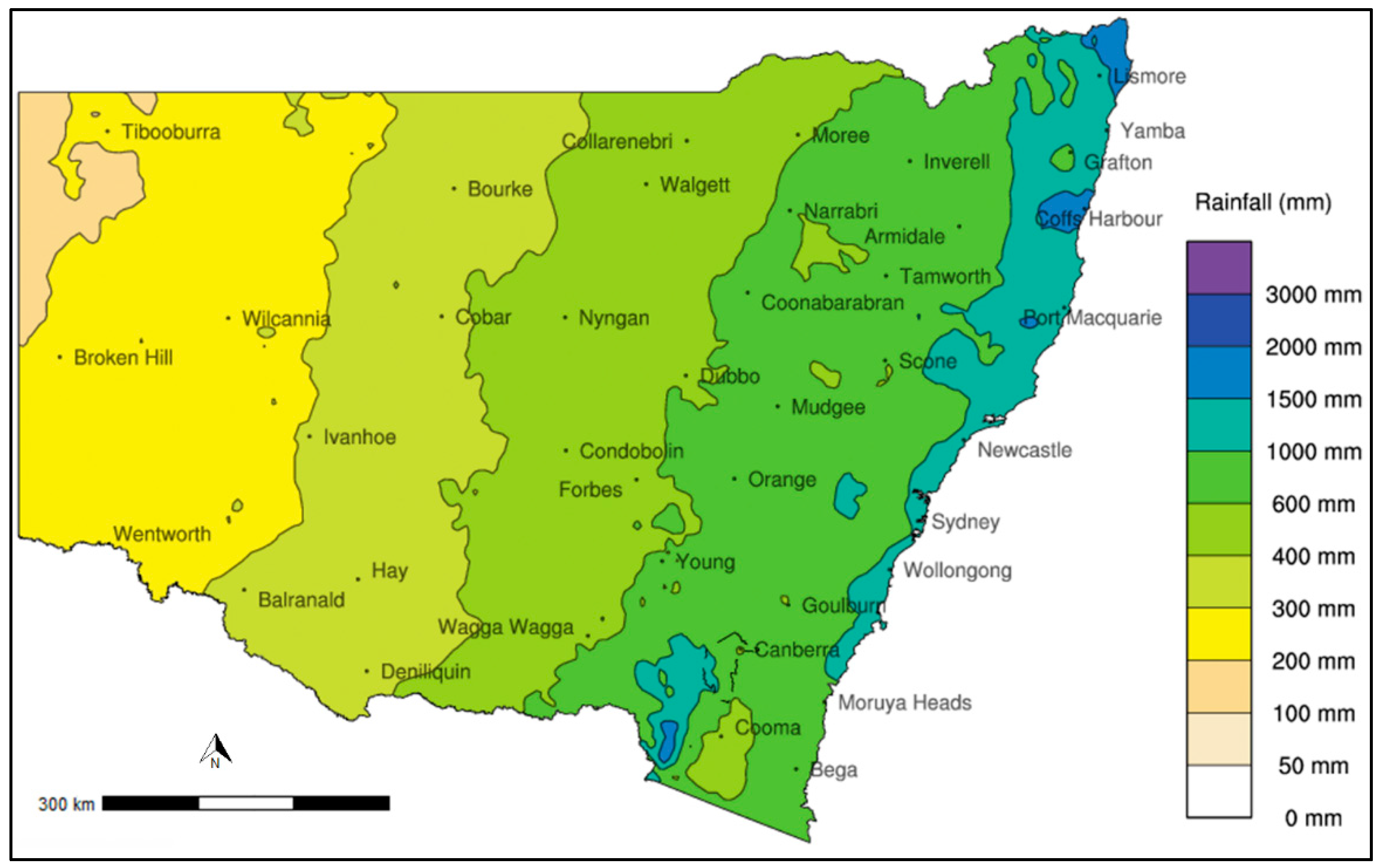
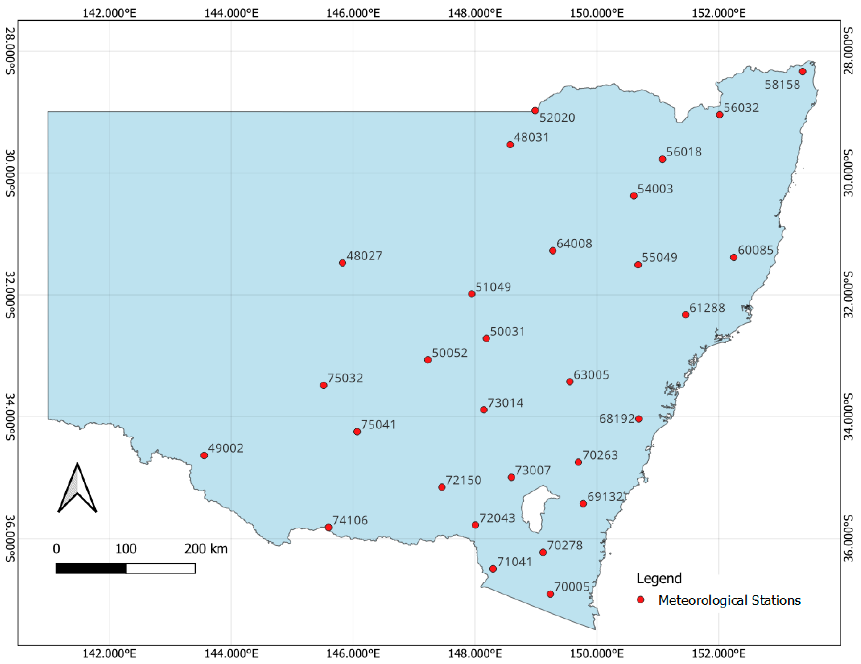
2.1. Study Area

To fulfill the objectives of this study, influences of climate change effects on design rainfall were assessed in NSW, Australia. NSW is surrounded by three other Australian states (Queensland to the north, Victoria to the south, and South Australia to the west), and the Tasman and Coral Seas. The state consists of mixed land use (residential, industrial, commercial, green, and open spaces) covering approximately 810,000 square kilometres. The elevation of the state is between −6 m and 2129 m.

More than half of the state is arid and semi-arid with annual mean rainfall ranging from 150 mm to 500 mm. For the study period (1900–2019), the daily extreme documented rainfall was 415.2 mm. Figure 1 shows the annual average rainfall for 30-year climatology (1991–2020) for NSW.

The northwest region of the state receives less rainfall compared with the eastern part as shown in Figure 1. As probable moisture sources are far from these areas, highly variable rainfall is observed. Due to the higher elevation in the north-western portion of the state, higher rainfall is observed in these areas. Average annual damage from floods in NSW amounts to approximately $250 million, although individual events can cause much more widespread damage, with the 2023 Lismore floods estimated to have caused nearly AUD 10 billion in damages. Anthropogenic climate change and associated consequences have the potential to increase the damage from increased extreme rainfall. A significant increase in the trend for short-duration extreme rainfall in NSW has already been observed by Hazani et al. [18]. As a result, the impacts of damage from flooding and associated costs of recovery will be further increased from aggravated extreme rainfall.

2.2. Rainfall Data

The objectives of this research were achieved using two daily rainfall data sets: historical observed rainfall data and projected rainfall data. Historical observed rainfall data (point data) from selected 29 weather stations were collected from the SILO database (https://www.longpaddock.qld.gov.au/silo/ (accessed on 1 August 2020)). Historical data were collected from the period of 1900 to 2019. As the data sets in the SILO are attained and stored from the BoM, which is the Australian Federal Government Organisation responsible for providing weather services across the country, and there were no missing data, these data sets were deemed appropriate for this research. The stations were selected to ensure a spread across the state. Figure 2 illustrates the locations of the selected meteorological stations in NSW.

Evaluation of the climate change influence on design rainfall for efficient stormwater management systems requires accurate evaluation of climate models [19,20]. Smith et al. [21] suggested three criteria for global climate model (GCM) selection. They include the long-term availability of projected data, spatially fine resolution of model data, and validity of model outputs using statistical techniques. In this research, future projected daily rainfall was collected from AdaptNSW (https://www.climatechange.environment.nsw.gov.au/climate-projections-used-adaptnsw (accessed on 1 August 2020). The data in AdaptNSW use the NARCLiM (NSW and Australian Regional Climate Modelling, Version 1.5) projections. The NSW government-led project, NARCLiM, generates detailed climate projections using scientifically reviewed methods and international best practices. As the projections from NARCLiM use internationally recognised GCMs, data from NARCLiM were used in this research. Data were accessed from this source and portioned into four future climate periods: 2020–2039, 2040–2059, 2060–2079, and 2080–2099.

As limitations exist in NARCLiM V1.0 (released in 2014), projected data from NARCLiM V1.5 were extracted and analysed to fulfill the objectives of this research. NARCLiM V1.5 is the second generation of NSW and Australian Regional Climate Modelling project for producing projected climate data in southeast Australia, i.e., at a regional scale. The projection of climate data in NARCLiM V1.5 is generated based on AR5 (5th Assessment Report) of the Intergovernmental Panel on Climate Change (IPCC). The spatial resolution of the collected data from NARCLiM V1.5 is 50 km for the emission scenario RCP4.5.

3. Methods

In this research, daily extreme rainfall was used to evaluate the influence of climate change effects on design rainfall. For the accomplishment of the objective, project rainfall from 2020 to 2099 was used, and probability of occurrence of extreme rainfall for different recurrence intervals was derived and compared with the value provided in the national guidelines from the Australian Bureau of Meteorology (BoM). The overall procedure can be summarised as follows:

• Collection and treatment of historical rainfall data;
• Collection and treatment of future rainfall data;
• Application of frequency analysis to the projected data;
• Evaluation of the outcomes with the current Australian standard.

The overall structure of the applied method is the same as the framework developed by Hossain et al. [22] and shown in Figure 3. However, Hossain et al.’s [22] study did not consider the systematic analysis and influence of data length in the design rainfall calculation.

The collected rainfall data from the NARCliM are in daily time step resolutions. Consequently, the derivation of extreme rainfall from daily data is the prerequisite for the frequency analysis. The block maxima (BM) approach and the peak over threshold (POT) approach are the commonly applied techniques in obtaining extreme value from time series data sets [10,23]. Amongst these two approaches, BM is the most frequently adopted technique in hydrological applications. In the BM approach, the annual maximum value from the available time series data is obtained. The barrier that most hinders the application of the POT series is the selection of the appropriate threshold value. If the threshold is too high, it will increase the variance in the data sets, whereas too low a threshold leads the data sets to be dependent on others [24]. As the BM technique is a simple and commonly employed technique in hydrologic applications, the method was applied for deriving extreme data sets in this study.

Determination of design rainfall for various recurrence intervals is usually obtained from the intensity–frequency–duration (IFD) curves/tables. As linear and non-linear models are not capable of estimating extreme vents [25], values of the IFD curves/tables are obtained by adopting conventional frequency analysis. Traditionally, frequency analysis is applied to understand the probability of occurrence of extreme events. As one or two statistical distributions are not able to demonstrate the complete temporal and spatial form of hydrological extremes, several statistical distributions are investigated by many researchers around the world. As a result, the conventional flood hazard analysis is performed by applying the general extreme value distribution (GEVD), which is the combination of three distributions.

In this study, the GEVD is fitted to historical and projected extreme rainfall for the selected meteorological stations in NSW, Australia. The traditional probability density function of the GEVD can be demonstrated by Equation (1), as adopted by many researchers [9,22,26].

$$f\left(x\right)=exp\left\{-\left[1+\xi {\left({\displaystyle \frac{y-\mu }{\sigma }}\right)}^{-{\displaystyle \frac{1}{\xi }}}\right]\right\}$$

(1)

where $\left\{y:1+\xi \left({\displaystyle \frac{y-\mu }{\sigma }}\right)>0\right\}$, $\mu , \sigma \mathrm{and} \xi$ are the location, scale, and shape parameters respectively for the GEVD.

Although numerous techniques for the estimation of GEVD are available in the literature, the L-moments method is a widely used technique for solving hydrologically extreme problems. Therefore, the L-moments method is adopted in this study.

The design rainfall depths using the GEVD were estimated by adopting the established Equation (2) [27]:

$$R_T=\left\{\begin{array}{c}\widehat{\mu }-{\displaystyle \frac{\widehat{\sigma }}{\widehat{\xi }}}\times \left[1-{\left(-log\left(1-p\right)\right)}^{\widehat{\xi }}\right] for \widehat{\xi }\ne 0\\ \widehat{\mu }-\widehat{\sigma }\times log\left(-log\left(1-p\right)\right) for \widehat{\xi }=0 \end{array}\right.$$

(2)

where $R_T$ is the rainfall depth for $T$ year return period, $T=1/p$.

4. Results and Discussion

This study evaluated the influence of climate change on design rainfall in NSW, Australia. The evaluation was first performed by determining the statistics of the extreme rainfall. Statistical comparison of the historical extreme rainfall with different time periods of projected rainfall is shown in

Table 1. Climate change effects on the statistics of extreme rainfall.

Station No.	2020–2039		2040–2059		2060–2079		2080–2099		1900–2019
	Maximum	CV	Maximum	CV	Maximum	CV	Maximum	CV	Maximum	CV
48027	125.11	0.34	98.38	0.31	111.33	0.52	130.81	0.42	113.20	0.45
48031	120.91	0.35	161.39	0.45	108.79	0.42	119.12	0.37	312.00	0.59
49002	44.16	0.35	44.44	0.36	68.46	0.45	38.04	0.26	93.30	0.43
50031	86.66	0.35	106.62	0.36	82.21	0.32	73.28	0.26	133.90	0.41
50052	68.73	0.31	76.78	0.34	85.82	0.34	81.06	0.32	127.20	0.42
51049	86.31	0.25	150.13	0.48	80.11	0.28	102.73	0.23	226.80	0.49
52020	101.70	0.33	111.52	0.42	109.11	0.44	154.79	0.52	208.00	0.42
54003	185.71	0.49	137.62	0.39	123.10	0.33	109.27	0.38	194.30	0.43
55049	117.31	0.30	138.16	0.40	135.37	0.34	125.91	0.37	136.70	0.32
56018	95.21	0.22	125.22	0.37	113.47	0.32	112.23	0.30	140.00	0.34
56032	89.60	0.25	67.93	0.23	89.10	0.37	98.44	0.35	190.60	0.40
58158	188.54	0.39	129.28	0.28	176.06	0.41	162.90	0.29	338.60	0.46
60085	128.96	0.24	144.40	0.26	183.05	0.38	240.75	0.40	415.20	0.46
61288	141.97	0.32	148.15	0.32	124.92	0.32	172.26	0.38	184.10	0.48
63005	66.49	0.19	72.50	0.29	83.64	0.29	73.73	0.23	108.70	0.36
64008	142.90	0.28	171.57	0.34	146.94	0.33	89.97	0.22	167.60	0.38
68192	107.43	0.30	138.77	0.44	115.01	0.38	117.78	0.36	198.70	0.47
69132	133.73	0.46	212.77	0.65	177.43	0.59	131.78	0.39	201.00	0.42
70005	89.92	0.34	93.59	0.35	81.69	0.34	105.24	0.47	249.40	0.49
70263	62.66	0.25	69.06	0.25	101.83	0.49	74.99	0.26	148.20	0.42
70278	86.47	0.33	74.22	0.34	75.47	0.31	124.61	0.51	107.20	0.39
71041	80.16	0.22	97.36	0.26	113.87	0.27	104.06	0.30	165.50	0.36
72043	92.24	0.20	98.90	0.28	116.75	0.27	90.84	0.26	164.60	0.34
72150	83.03	0.35	70.76	0.27	93.14	0.38	68.07	0.29	110.80	0.40
73007	66.52	0.18	102.00	0.34	90.15	0.27	88.98	0.30	162.50	0.45
73014	85.59	0.28	90.73	0.36	130.08	0.49	101.72	0.30	110.70	0.35
74106	62.56	0.30	69.03	0.32	78.21	0.43	75.92	0.40	117.70	0.41
75032	111.85	0.54	68.42	0.32	66.15	0.32	105.71	0.51	123.00	0.46
75041	101.94	0.46	71.44	0.32	69.18	0.31	57.09	0.28	149.80	0.53

.

It is obvious from Table 1 that the GCM model underestimates the extreme rainfall compared with the historical observations. For example, observed extreme rainfall in station #48031 was 312 mm, whereas the projected rainfall for the same station was 120.91 mm, 161.39 mm, 108.79 mm, and 119.12 for the periods of 2020–2039, 2040–2059, 2060–2079, and 2080–2099 respectively. This statement is true for most of the stations. In addition, there is a variation in the extreme rainfall in the project data with time periods. The coefficient of variation (CV) was applied to identify the overall precision of extreme data sets. From Table 1, it is apparent that the CV for most of the stations was higher for the historical extreme rainfall contrasting with extreme values of the projected rainfall. Consequently, projected extreme rainfall shows relatively lower variability in the mean compared with the historical extreme rainfall. This could be one of the main reasons for having a higher extreme value for historical rainfall.

The geographic features of the area, climatic patterns, and local weather conditions are the probable reasons for such high spatial variations. Areas near the coast usually have higher extreme rainfall compared to the inland due to moisture-laden winds from the Pacific Ocean. The average annual rainfall for the latest 30-year climatology (1991 to 2020) was also higher near the coast, as shown in Figure 1. Therefore, historical maximum extreme rainfall (415.20 mm) and minimum (93.30 mm) were observed near to the coastal and inland stations, respectively, as illustrated in Table 1. Moreover, the combined influence of La Niña and negative Indian Ocean Dipole (IOD) has a substantial impact on the extreme rainfall throughout eastern Australia [28]. As the influence of oceanic temperature variation (e.g., La Niña, IOD, etc.) is not the same across the state, the spatial variation in extreme rainfall is significant. In addition, tropical cyclones and thunderstorms, which vary across NSW, have considerable influence on the spatial variability of extreme rainfall, as shown in Table 1.

Likelihood estimation of parameters for GEVD is essential for the determination of the probability of exceedance of design rainfall. Although different parameter estimation techniques of the GEVD could be found in the literature, the L-moment parameters estimation technique is commonly used in the design rainfall estimation [26]. Also, estimation of design rainfall in Australia BoM applied the L-moments technique. Therefore, the method has been applied in this research to estimate the parameters of the GEVD. The estimated shape parameters for all the meteorological stations are shown in

Table 2. Climate change effects on the shape parameter of the GEV distribution.

Station #	1900 to 2019	1920 to 2039	1940 to 2059	1960 to 2079	1980 to 2099
48027	0.1	0.0	0.0	0.2	0.0
48031	0.2	−0.2	0.4	−0.1	0.0
49002	0.0	0.0	−0.1	0.2	−0.2
50031	0.1	−0.1	0.2	−0.2	−0.2
50052	0.0	−0.1	−0.2	0.0	0.0
51049	0.1	−0.4	0.1	−0.4	0.0
52020	0.1	0.0	0.1	0.1	0.2
54003	0.1	0.4	0.2	0.1	0.1
55049	0.0	0.1	0.2	0.1	0.1
56018	0.0	−0.1	0.1	0.1	−0.1
56032	0.2	0.1	−0.7	0.0	0.0
58158	0.0	0.1	−0.1	0.0	0.1
60085	0.1	−0.3	0.0	0.2	0.3
61288	0.2	0.0	0.2	−0.1	0.1
63005	0.0	0.0	−0.1	0.1	0.0
64008	0.1	−0.3	0.1	0.0	−0.2
68192	0.2	−0.1	0.0	0.1	0.0
69132	0.1	0.2	0.3	0.4	0.0
70005	0.2	0.0	−0.2	−0.2	0.2
70263	0.2	−0.3	0.0	0.0	−0.2
70278	0.1	0.0	−0.1	0.0	0.4
71041	0.1	−0.1	0.2	0.0	−0.1
72043	0.0	−0.1	0.0	0.1	0.0
72150	0.2	0.1	0.0	0.3	−0.3
73007	0.2	−0.4	−0.1	0.2	−0.4
73014	0.0	0.1	0.1	0.2	0.0
74106	0.1	0.1	−0.3	0.2	0.0
75032	0.1	0.4	−0.1	−0.2	0.4
75041	0.2	0.3	−0.2	−0.3	−0.1

.

The analysis of the research found that the shape parameter of the GEVD is either zero or positive for historical rainfall. Therefore, the distribution is either Gumbel type (for zero shape parameter) type or Fréchet (for positive shape parameter) distribution. However, for the extreme data of the projected rainfall, the distribution may be either Gumbel or Fréchet or Weibull (for negative shape parameter). Nevertheless, there is inconsistency in the distribution type amongst the data sets. For example, the historical extreme rainfall data set for station #48027 follows the Fréchet type distribution. On the other hand, the same station follows the Gumbel type distribution for the period of 1920 to 2039, 1940 to 2059, and 1980 to 2099, and the Fréchet type distribution for the period of 1960 to 2079. This may be due to the potential climate change variables considered for deriving the projected rainfall.

Estimation of return levels for different recurrence intervals for both historical and projected extreme rainfall are shown in

Table 3. Variation in Return Level due to Climate Change NSW, Australia.

a. Variation in Return Level due to Climate Change NSW, Australia.
Station #	1900 to 2019										2020 to 2039
	2 Yr		5 Yr		10 Yr	20 Yr	50 Yr		100 Yr		2 Yr	5 Yr	10 Yr		20 Yr	50 Yr		100 Yr
48027	38.5		54.9		66.8	79.0	96.3		110.3		57.9	76.6	89.6		102.4	119.7		133.1
48031	53.5		78.7		100.9	127.7	172.4		215.4		62.8	83.8	95.7		106.0	117.6		125.2
49002	35.5		50.1		59.8	69.3	81.7		91.1		22.1	29.6	34.7		39.7	46.3		51.3
50031	51.9		72.1		86.5	101.1	121.1		137.1		51.9	69.5	80.2		89.8	101.4		109.5
50052	40.5		56.2		66.4	75.9	88.0		96.8		41.2	53.9	61.8		69.1	78.2		84.6
51049	45.1		63.3		78.0	94.5	120.0		142.7		63.9	77.1	82.9		86.9	90.5		92.4
52020	56.3		77.9		92.9	107.8	127.9		143.6		56.4	74.9	87.3		99.2	114.9		126.8
54003	55.1		75.2		91.5	109.7	137.8		162.8		54.2	71.1	87.8		109.8	150.7		194.2
55049	54.4		70.9		81.9	92.5	106.4		116.9		60.7	78.7	91.5		104.6	122.8		137.4
56018	56.5		74.5		87.0	99.3	116.0		128.9		62.1	75.4	83.7		91.3	100.6		107.2
56032	60.3		83.1		100.1	117.9	143.6		164.8		49.0	60.7	68.8		76.9	87.8		96.4
58158	135.1		196.3		237.7	277.9	331.0		371.4		86.6	119.0	143.0		168.1	204.0		233.7
60065	109.2		156.2		189.9	224.3	272.0		310.3		91.9	111.9	122.3		130.4	139.0		144.1
61288	61.7		90.8		112.6	135.8	169.5		197.8		75.7	98.9	114.1		128.5	147.0		160.7
63005	45.5		60.9		71.8	82.8	97.8		109.7		44.9	53.0	58.3		63.4	69.9		74.7
64008	65.4		89.3		106.3	123.7	147.8		167.1		86.4	108.1	119.4		128.4	137.8		143.5
68192	69.7		101.8		125.7	150.7	186.6		216.3		62.1	79.9	90.1		98.9	109.0		115.7
69132	64.3		88.8		106.3	123.9	148.3		167.7		56.2	82.6	103.0		125.1	157.9		186.0
70005	54.7		76.7		94.1	113.4	142.6		168.2		44.3	58.7	68.2		77.1	88.5		97.0
70263	52.0		72.2		87.8	104.6	129.4		150.6		44.3	54.2	59.3		63.3	67.4		69.9
70278	44.8		61.9		73.7	85.2	100.7		112.6		45.7	60.7	70.5		79.8	91.7		100.5
71041	67.4		90.6		107.0	123.6	146.3		164.4		53.7	65.1	72.0		78.2	85.6		90.8
72043	53.8		70.2		81.5	92.9	108.3		120.2		63.2	75.4	82.8		89.3	97.0		102.3
72150	39.9		54.6		65.9	78.3	96.6		112.4		40.1	53.8	63.9		74.4	89.2		101.4
73007	53.9		75.3		93.0	113.3	145.3		174.4		50.9	58.6	62.2		64.8	67.3		68.6
73014	50.2		67.3		78.4	88.7	101.8		111.4		48.6	61.3	70.6		80.2	93.7		104.8
74106	38.9		53.9		64.2	74.5	88.2		98.9		34.3	44.3	51.7		59.4	70.4		79.5
75032	39.0		55.7		67.8	80.3	97.9		112.1		33.4	47.3	61.1		79.2	112.6		148.0
75041	32.5		46.7		58.6	72.4	94.4		114.7		35.8	50.1	62.9		78.4	104.6		130.2
b. Variation of Return Level due to Climate Change NSW, Australia.
Station #	2040 to 2059						2060 to 2079						2080 to 2099
	2 Yr	5 Yr	10 Yr	20 Yr	50 Yr	100 Yr	2 Yr	5 Yr	10 Yr	20 Yr	50 Yr	100 Yr	2 Yr	5 Yr	10 Yr	20 Yr	50 Yr	100 Yr
48027	52.1	68.1	79.1	89.8	104.0	114.9	42.4	65.0	83.0	103.1	133.8	160.9	56.6	79.9	95.7	111.2	131.7	147.4
48031	57.2	79.2	99.4	124.5	168.0	211.3	55.9	79.3	93.3	105.8	120.7	131.0	63.1	85.5	99.7	112.9	129.2	141.1
49002	24.0	32.4	37.2	41.4	46.2	49.4	26.9	38.9	48.1	58.1	73.0	85.7	24.2	30.0	33.0	35.4	37.9	39.5
50031	48.6	65.1	78.0	92.1	113.4	131.9	47.7	62.1	70.1	76.7	84.0	88.7	50.9	63.0	69.5	74.7	80.4	83.9
50052	44.7	59.1	67.2	74.2	82.1	87.3	40.6	53.8	62.6	71.2	82.3	90.7	43.4	56.8	66.0	75.0	86.9	96.1
51049	51.4	73.9	90.5	107.9	132.9	153.4	56.8	70.1	76.3	80.7	84.9	87.2	60.1	73.3	82.3	91.0	102.5	111.3
52020	50.8	72.1	87.2	102.4	123.3	139.8	52.1	75.3	91.9	108.8	132.1	150.8	54.7	82.6	104.8	129.2	166.1	198.4
54003	52.7	70.1	84.5	101.0	127.2	151.0	55.5	72.2	84.0	95.8	112.0	124.7	56.9	78.5	94.0	109.8	131.7	149.4
55049	60.0	83.5	101.5	121.0	149.7	174.3	64.5	85.2	99.6	114.0	133.4	148.6	58.2	78.9	93.9	109.2	130.5	147.7
56018	59.5	81.0	96.2	111.6	132.5	149.1	58.9	76.9	89.9	103.5	122.5	138.0	62.4	80.6	91.6	101.4	113.0	121.0
56032	54.0	62.6	65.7	67.5	68.9	69.5	50.8	69.7	81.7	92.9	106.9	117.1	53.6	72.1	84.9	97.4	114.2	127.3
58158	78.8	100.2	113.3	125.0	139.1	148.9	76.7	106.8	126.2	144.5	167.6	184.5	80.5	101.6	116.6	131.9	153.0	169.8
60065	75.0	92.3	103.7	114.6	128.8	139.4	77.0	105.0	126.6	150.1	185.1	215.2	92.0	123.1	150.6	183.7	239.0	292.2
61288	67.7	87.4	103.1	120.6	147.4	171.0	77.1	101.7	116.7	130.3	146.6	157.9	77.6	106.7	128.8	152.5	187.0	216.2
63005	44.7	57.6	65.6	72.9	81.9	88.2	43.8	55.9	64.7	73.6	86.1	96.1	47.6	58.2	64.9	71.2	79.1	84.9
64008	76.2	99.3	116.6	135.0	161.5	183.7	68.7	88.8	102.7	116.6	135.3	149.9	63.5	76.5	83.6	89.5	95.9	100.0
68192	62.2	89.8	108.6	127.1	151.8	170.7	54.8	75.2	90.1	105.4	126.9	144.3	61.2	82.5	96.8	110.7	129.0	142.9
69132	54.8	88.7	119.2	156.6	220.3	282.7	54.0	81.5	108.6	144.2	210.0	279.5	64.0	89.3	106.5	123.4	146.0	163.3
70005	54.0	71.3	80.6	88.3	96.7	102.0	49.1	64.6	73.1	80.1	87.7	92.5	42.9	62.8	78.6	96.0	122.3	145.2
70263	46.0	57.2	64.6	71.8	81.1	88.1	48.8	73.4	89.6	105.2	125.2	140.2	46.4	57.7	64.0	69.3	75.3	79.2
70278	45.1	60.4	69.9	78.5	88.9	96.3	42.9	56.2	65.3	74.3	86.5	96.0	39.0	55.7	71.3	90.9	125.1	159.5
71041	53.6	66.7	76.8	87.9	104.3	118.5	63.0	78.7	88.6	97.8	109.3	117.5	54.9	70.4	79.8	88.3	98.4	105.5
72043	56.2	71.6	82.0	92.1	105.5	115.7	65.4	82.5	95.1	108.2	126.9	142.4	58.9	73.8	83.3	92.2	103.3	111.4
72150	42.7	54.0	61.3	68.0	76.5	82.6	44.1	59.1	72.1	87.3	112.2	135.5	43.3	54.6	60.2	64.6	69.0	71.6
73007	50.6	67.1	77.2	86.5	97.7	105.6	46.6	57.6	66.1	75.1	88.5	99.8	59.8	74.9	81.8	86.9	91.6	94.2
73014	43.6	58.6	69.2	79.7	94.0	105.1	45.0	65.9	83.2	103.1	134.7	163.5	53.1	68.5	78.4	87.7	99.4	108.0
74106	39.7	50.7	56.4	60.8	65.4	68.2	33.2	46.2	56.8	68.8	87.3	104.0	33.4	46.4	55.1	63.5	74.4	82.6
75032	38.7	50.6	57.5	63.4	70.2	74.8	40.3	52.1	58.5	63.8	69.6	73.3	31.9	44.5	56.8	72.8	102.2	133.1
75041	44.3	57.5	64.4	70.0	75.8	79.4	45.4	58.1	64.4	69.2	74.1	77.0	36.2	46.0	52.1	57.7	64.5	69.3

a,b. The comparison provides information for the rainfall depth for 2-year, 5-year, 10-year, 20-year, 50-year, and 100-year return periods for a 24-hour duration. For this duration, the rainfall depth increases as the return period increases. However, there exists variation in the estimated depths between the historical and projected extreme rainfall.

A visual representation of the comparison for the return level estimation is shown in Figure 4 in the form of a heatmap. In Figure 4, station numbers are shown in rows and recurrence intervals are shown in columns. The dark colour represents the higher value, and the light colour represents the lower value. The hierarchical dendrogram of the heatmap is shown on the left side (illustrated by lines) of the colour map using average linkage and clearing distance. Figure 4 demonstrates that the rainfall stations are grouped according to the number of similar magnitudes of design rainfall for different recurrence intervals. The number of higher magnitudes of design rainfall for stations #58158 and #60065 are relatively greater compared with the other stations, indicating the spatial discrepancy of the extreme rainfall. That is why these stations are put together at the bottom of the Figure. A similar explanation is applicable for the stations (#710 and #73007) with the lower magnitudes of design rainfall as depicted in Figure 4.

For most of the meteorological stations, the probability of occurrence of projected rainfall is lower than the historical rainfall. In several stations, substantial variation was identified. There is also significant variation amongst the projection periods. For example, the 100-year return level for station #48031 is 172.4 mm. However, 100-year return levels for the same station are 125.2 mm, 211.3 mm, 131.0, and 141.1 mm for the periods of 2020 to 2039, 2040 to 2059, 2060 to 2079, and 2080 to 2099, respectively, as shown in Table 3a,b. This variation is due to the climate change impacts on the design rainfall. Influences of climate change were not considered in determining the design rainfall. Projected rainfall is determined by considering different emission scenarios for different time periods. Intrinsically, 312 mm of historical extreme rainfall was observed for station #48031, whereas 120.91 mm, 161.39 mm, 108.79 mm, and 119.12 mm rainfall was considered for the periods of 2020–2039, 2040–2059, 2060–2079, and 2080–2099.

Similar findings were observed in previous studies where different rainfall depths and intensities were derived from the climate modelling outputs [29,30]. Simonovic and Peck [31] also derived higher rainfall depth for the higher recurrence intervals from the historical extreme rainfall compared with projected rainfall. Therefore, extreme rainfall in NSW will be significantly affected by climate change, and, hence, estimation of design rainfall that is used for stormwater management infrastructures design should adopt impacts of climate change.

Further comparison of the climate change impacts on the design rainfall is shown in Figure 5. The assessment is shown between the design rainfall derived from the extreme data of the projected rainfall and the design rainfall from the Australian BoM for the same meteorological stations. It should be noted that the derivation of design rainfall by Australian BoM did not consider the influence of climate change. The daily design rainfall due to potential climate change in NSW will decrease as illustrated in Figure 5 for the selected four stations. An analogous trend was observed for other meteorological stations as well. Apparently, significant influences exist on the design rainfall due to climate change and the design rainfall in NSW will decrease from probable climate change. However, the magnitude of the changes depends on the length of the data periods, as shown in Figure 5. A similar observation was also found by Khastagir et al. [32]. In addition, the variation in the magnitude is higher for the high recurrence intervals and lower for the low recurrence interval, as revealed in Figure 5. The findings are also coherent with the findings examined by Meresa et al. [33].

The number of stations showing decreased or increased design rainfall compared to the ARR design rainfall is shown in Table 3. The number of stations showing decreased design rainfall is similar for all the future rainfall design rainfall scenarios. The maximum number of stations showing increased design rainfall is in the 2080–2099 design rainfall scenarios for the 100-year event. Therefore, the potential future design rainfall for 24 h duration will be decreased in most of the areas in NSW, as demonstrated in Table 3.

The outcomes of the study suggested that future rainfall intensity will cause decreased peak runoff and flood potentiality in NSW. It is well-known that stormwater management infrastructures are designed based on design rainfall derived from historic extreme rainfall. This assumption leads to under-design or over-design due to climate change and the consequences of the shift in frequency and occurrence of extreme rainfall. Furthermore, the design rainfall obtained from projected extreme rainfall will make this system uncertain for future stormwater management. However, inconsistent observations were found by other researchers. For example, Kundzewicz et al. [34], Nile et al. [35], and Hassan et al. [36] found increased severity and risks of flooding due to increased extreme rainfall from climate change. The reason for the dissimilar observation may be due to the changes in the geographic regions. In contrast, the outcomes of this study are consistent with the research performed in similar geographical locations [37]. Therefore, it is essential to understand the influence of climate change impacts on design rainfall estimation on a regional scale. The findings of this research have the potential to address risks and uncertainty arising from inadequate drainage systems.

It is worth noting that the selection of the number of extreme data points substantially impacts the modelling outcomes. As the extreme data sets for projected rainfall were estimated from data from a twenty year period, there is the potential for a more stable and reliable parameter estimation of the GEV distribution. Furthermore, fewer extreme values (20 from 20 years) can reduce the sensitivity of the outliers, which may alter the approximation of extreme quantiles. In addition, a lesser number of extreme values help avoid the overfitting of the GEV method. However, a lesser number of extreme values may represent the tail behaviour of the distribution, inaccurately leading to misinterpretation of the extreme value theory. There may be bias in the magnitude of the estimated parameters, leading to a reduction in the predictive capability of the methods. Hence, the selection of appropriate block length is a balance between extracting sufficient extreme data points to fit the GEV distribution accurately and preventing the demise of suitable information or unnecessary computational difficulty.

5. Conclusions and Recommendations

In this research, the impacts of climate change on daily design rainfall in NSW, Australia have been investigated. Daily observed rainfall from 1900 to 2019 and rainfall outputs for different time periods (2020 to 2039, 2040 to 2059, 2060 to 2079, and 2080 to 2099) from GCM (CSIRO BOM ACCESS 3.0) were analysed to derive design rainfall. For the assessment of computed design rainfall from the GCM, projected rainfall was compared with the design rainfall from the Australian BoM. Based on the outcomes of this study, the following general conclusions can be drawn:

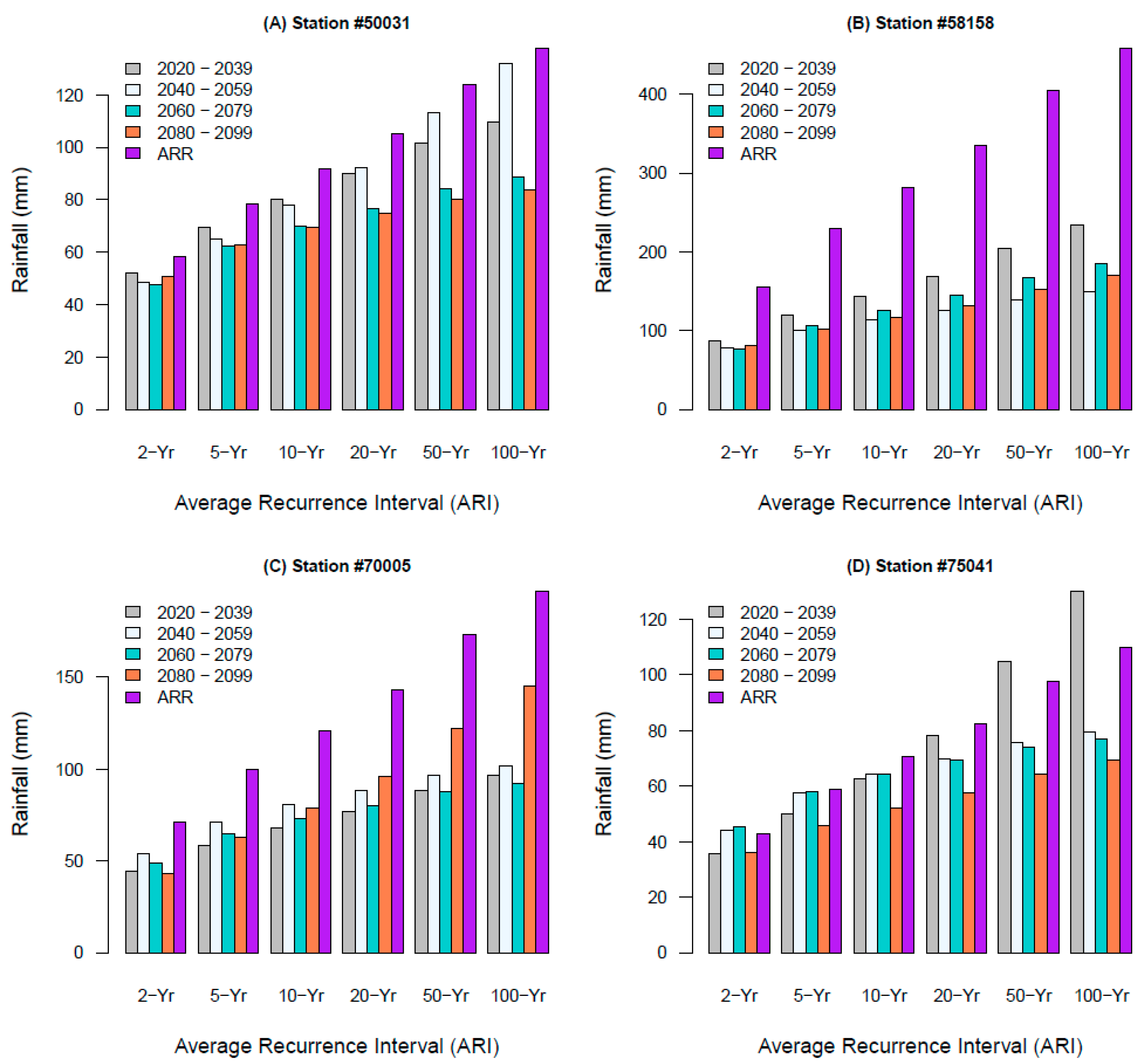
• Design rainfall in most parts of NSW will be significantly impacted by climate change impacts; however, the magnitude of changes varies amongst the recurrence intervals.
• Most of the regions in NSW will be facing decreased rainfall from climate change, leading to potential drought.
• The decrease in design rainfall for 100 years recurrence interval ranges from 2.5% to 67.6%, whereas the increase in design rainfall would be between 1.2% to 35.9%. This outcome changes with the changes in the data periods. Nevertheless, a decrease in design rainfall was observed for most of the areas.
• Stormwater drainage systems designed considering historical rainfall will be under-designed or over-designed, leading to uncertainty in flood mitigation. The extent of this uncertainty depends on climate models and return periods.

The selection of block size for the extraction of maxima is subjective leading to the uncertainty of the magnitude of the parameters of the GEV distribution. The use of different numbers of extreme data points has the potential to significantly impact the interpretation of extreme value analysis. The properties of the data, definite aims of the study, and practical considerations should be given priority in selecting the number of extreme data for GEV analysis.

For a generic conclusion, advanced investigation is required for the accurate derivation of design rainfall required for the design of stormwater infrastructures in NSW. The standard and guideline for the extraction of design rainfall from the Australian BoM should be revised to encompass climate change impacts. It is worth noting that the investigation of this research is performed on daily extreme rainfall. Additionally, analysis of sub-daily rainfall data should be performed for an improved understanding of climate change.

References

1. Bibi, T.S.; Tekesa, N.W. Impacts of climate change on IDF curves for urban stormwater management systems design: The case of Dodola Town, Ethiopia. Environ. Monit. Assess. 2023, 195, 170. [Google Scholar] [CrossRef] [PubMed]
2. Cook, L.M.; McGinnis, S.; Samaras, C. The effect of modeling choices on updating intensity-duration-frequency curves and stormwater infrastructure designs for climate change. Clim. Chang. 2020, 159, 289–308. [Google Scholar] [CrossRef]
3. Bulti, D.T.; Abebe, B.G.; Biru, Z. Climate change–induced variations in future extreme precipitation intensity–duration–frequency in flood-prone city of Adama, central Ethiopia. Environ. Monit. Assess. 2021, 193, 784. [Google Scholar] [CrossRef] [PubMed]
4. Butcher, J.B.; Zi, T.; Pickard, B.R.; Job, S.C.; Johnson, T.E.; Groza, B.A. Efficient statistical approach to develop intensity-duration-frequency curves for precipitation and runoff under future climate. Clim. Chang. 2021, 164, 3. [Google Scholar] [CrossRef] [PubMed]
5. Tousi, E.G.; O’Brien, W.; Doulabian, S.; Toosi, A.S. Climate changes impact on stormwater infrastructure design in Tucson Arizona. Sustain. Cities Soc. 2021, 72, 103014. [Google Scholar] [CrossRef]
6. Fadhel, S.; Rico-Ramirez, M.A.; Han, D. Uncertainty of intensity–duration–frequency (IDF) curves due to varied climate baseline periods. J. Hydrol. 2017, 547, 600–612. [Google Scholar] [CrossRef]
7. Hettiarachchi, S.; Wasko, C.; Sharma, A. Increase in flood risk resulting from climate change in a developed urban watershed–the role of storm temporal patterns. Hydrol. Earth Syst. Sci. 2018, 22, 2041–2056. [Google Scholar] [CrossRef]
8. Myhre, G.; Alterskjær, K.; Stjern, C.W.; Hodnebrog, Ø.; Marelle, L.; Samset, B.H.; Sillmann, J.; Schaller, N.; Fischer, E.; Schulz, M. Frequency of extreme precipitation increases extensively with event rareness under global warming. Sci. Rep. 2019, 9, 16063. [Google Scholar] [CrossRef]
9. Yilmaz, A.G.; Hossain, I.; Perera, B.J.C. Effect of climate change and variability on extreme rainfall intensity–frequency–duration relationships: A case study of Melbourne. Hydrol. Earth Syst. Sci. 2014, 18, 4065–4076. [Google Scholar] [CrossRef]
10. Yilmaz, A.G.; Perera, B.J.C. Extreme Rainfall Nonstationarity Investigation and Intensity–Frequency–Duration Relationship. J. Hydrol. Eng. 2014, 19, 1160–1172. [Google Scholar] [CrossRef]
11. Mirhosseini, G.; Srivastava, P.; Stefanova, L. The impact of climate change on rainfall Intensity–Duration–Frequency (IDF) curves in Alabama. Reg. Environ. Chang. 2013, 13, 25–33. [Google Scholar] [CrossRef]
12. Rosenberg, E.A.; Keys, P.W.; Booth, D.B.; Hartley, D.; Burkey, J.; Steinemann, A.C.; Lettenmaier, D.P. Precipitation extremes and the impacts of climate change on stormwater infrastructure in Washington State. Clim. Chang. 2010, 102, 319–349. [Google Scholar] [CrossRef]
13. Fowler, H.J.; Wasko, C.; Prein, A.F. Intensification of short-duration rainfall extremes and implications for flood risk: Current state of the art and future directions. Philos. Trans. R. Soc. A 2021, 379, 20190541. [Google Scholar] [CrossRef] [PubMed]
14. Kourtis, I.M.; Tsihrintzis, V.A. Update of intensity-duration-frequency (IDF) curves under climate change: A review. Water Supply 2022, 22, 4951–4974. [Google Scholar] [CrossRef]
15. Liang, C.; Li, D.; Yuan, Z.; Liao, Y.; Nie, X.; Huang, B.; Wu, X.; Xie, Z. Assessing urban flood and drought risks under climate change, China. Hydrol. Process. 2019, 33, 1349–1361. [Google Scholar] [CrossRef]
16. CSIRO. State of the Climate 2020; Australian Bureau of Meteorology: Melbourne, Australia, 2020; p. 1486315097.
17. Australian Bureau of Meteorology. 2022. Available online: http://www.bom.gov.au/climate/data/?ref=ftr (accessed on 1 November 2021).
18. Hajani, E.; Rahman, A.; Ishak, E. Trends in extreme rainfall in the state of New South Wales, Australia. Hydrol. Sci. J. 2017, 62, 2160–2174. [Google Scholar] [CrossRef]
19. Gu, H.; Yu, Z.; Wang, G.; Wang, J.; Ju, Q.; Yang, C.; Fan, C. Impact of climate change on hydrological extremes in the Yangtze River Basin, China. Stoch. Environ. Res. Risk Assess. 2015, 29, 693–707. [Google Scholar] [CrossRef]
20. Sun, X.; Li, R.; Shan, X.; Xu, H.; Wang, J. Assessment of climate change impacts and urban flood management schemes in central Shanghai. Int. J. Disaster Risk Reduct. 2021, 65, 102563. [Google Scholar] [CrossRef]
21. Smith, D.M.; Kniveton, D.R.; Barrett, E.C. A statistical modeling approach to passive microwave rainfall retrieval. J. Appl. Meteorol. Climatol. 1998, 37, 135–154. [Google Scholar] [CrossRef]
22. Hossain, I.; Imteaz, M.; Gato-Trinidad, S.; Yilmaz, A.G. Comparison of Future Design Rainfall with Current Design Rainfall: A Case Study in New South Wales, Australia. Atmosphere 2024, 15, 739. [Google Scholar] [CrossRef]
23. Wi, S.; Valdés, J.B.; Steinschneider, S.; Kim, T.-W. Non-stationary frequency analysis of extreme precipitation in South Korea using peaks-over-threshold and annual maxima. Stoch. Environ. Res. Risk Assess. 2016, 30, 583–606. [Google Scholar] [CrossRef]
24. Sane, Y.; Panthou, G.; Bodian, A.; Vischel, T.; Lebel, T.; Dacosta, H.; Quantin, G.; Wilcox, C.; Ndiaye, O.; Diongue-Niang, A. Intensity–duration–frequency (IDF) rainfall curves in Senegal. Nat. Hazards Earth Syst. Sci. 2018, 18, 1849–1866. [Google Scholar] [CrossRef]
25. Hossain, I.; Rasel, H.M.; Imteaz, M.A.; Mekanik, F. Long-term seasonal rainfall forecasting: Efficiency of linear modelling technique. Environ. Earth Sci. 2018, 77, 280. [Google Scholar] [CrossRef]
26. Hossain, I.; Imteaz, M.A.; Khastagir, A. Effects of estimation techniques on generalised extreme value distribution (GEVD) parameters and their spatio-temporal variations. Stoch. Environ. Res. Risk Assess. 2021, 35, 2303–2312. [Google Scholar] [CrossRef]
27. Alam, M.A.; Emura, K.; Farnham, C.; Yuan, J. Best-fit probability distributions and return periods for maximum monthly rainfall in Bangladesh. Climate 2018, 6, 9. [Google Scholar] [CrossRef]
28. Hossain, I.; Esha, R.; Alam Imteaz, M. An Attempt to Use Non-Linear Regression Modelling Technique in Long-Term Seasonal Rainfall Forecasting for Australian Capital Territory. Geosciences 2018, 8, 282. [Google Scholar] [CrossRef]
29. Alam, M.S.; Elshorbagy, A. Quantification of the climate change-induced variations in Intensity–Duration–Frequency curves in the Canadian Prairies. J. Hydrol. 2015, 527, 990–1005. [Google Scholar] [CrossRef]
30. DeGaetano, A.T.; Castellano, C.M. Future projections of extreme precipitation intensity-duration-frequency curves for climate adaptation planning in New York State. Clim. Serv. 2017, 5, 23–35. [Google Scholar] [CrossRef]
31. Simonovic, S.P.; Peck, A. Updated Rainfall Intensity Duration Frequency Curves for the City of London under the Changing Climate; Department of Civil and Environmental Engineering, The University of Western Ontario: London, ON, Canada, 2009. [Google Scholar]
32. Khastagir, A.; Hossain, I.; Aktar, N. Evaluation of different parameter estimation techniques in extreme bushfire modelling for Victoria, Australia. Urban. Clim. 2021, 37, 100862. [Google Scholar] [CrossRef]
33. Meresa, H.; Tischbein, B.; Mekonnen, T. Climate change impact on extreme precipitation and peak flood magnitude and frequency: Observations from CMIP6 and hydrological models. Nat. Hazards 2022, 111, 2649–2679. [Google Scholar] [CrossRef]
34. Kundzewicz, Z.W.; Kanae, S.; Seneviratne, S.I.; Handmer, J.; Nicholls, N.; Peduzzi, P.; Mechler, R.; Bouwer, L.M.; Arnell, N.; Mach, K. Flood risk and climate change: Global and regional perspectives. Hydrol. Sci. J. 2014, 59, 1–28. [Google Scholar] [CrossRef]
35. Nile, B.K.; Hassan, W.H.; Alshama, G.A. Analysis of the effect of climate change on rainfall intensity and expected flooding by using ANN and SWMM programs. ARPN J. Eng. Appl. Sci. 2019, 14, 974–984. [Google Scholar]
36. Hassan, W.H.; Nile, B.K.; Al-Masody, B.A. Climate change effect on storm drainage networks by storm water management model. Environ. Eng. Res. 2017, 22, 393–400. [Google Scholar] [CrossRef]
37. Li, J.; Evans, J.; Johnson, F.; Sharma, A. A comparison of methods for estimating climate change impact on design rainfall using a high-resolution RCM. J. Hydrol. 2017, 547, 413–427. [Google Scholar] [CrossRef]
Figure 1. Annual average rainfall for NSW over the 1991–2020 period.
Atmosphere 15 01101 g001
Figure 2. The relative position of the rainfall stations in NSW, Australia that were used to generate future scenarios of design rainfall due to upcoming climate change.
Atmosphere 15 01101 g002
Figure 3. Framework for identifying the influence of climate change effects on design rainfall [22]. The processes inside the red dotted box are performed by the Australian Bureau of Meteorology. The blue arrows show how the process progresses from one step to the next.
Atmosphere 15 01101 g003
Figure 4. Visual representation of return level estimation for different recurrence intervals for all the periods of extreme rainfall. Symbols ‘a’ represents 1900–2019, ‘b’ represents 2020–2039, ‘c’ represents 2040–2059, ‘d’ represents 2060–2079, and ‘e’ represents 2080–2099. The lines on the left of the figure represent the dendrogram which shows the structure of the cluster for rainfall stations.
Atmosphere 15 01101 g004
Figure 5. Design rainfall comparison between ARR and projected rainfall for different time periods for four selected meteorological stations. The symbols (AD) are for different meteorological stations as shown.
Atmosphere 15 01101 g005