Article

Feasibility Study of Microwave Radiometer Neural Network Modeling Method Based on Reanalysis Data

China Research Institute of Radiowave Propagation, Qingdao 266107, China
*
Author to whom correspondence should be addressed.
Atmosphere 2025, 16(10), 1194; https://doi.org/10.3390/atmos16101194
Submission received: 18 August 2025 / Revised: 10 October 2025 / Accepted: 10 October 2025 / Published: 16 October 2025

Abstract

To address the challenge of microwave radiometer modeling in regions lacking radiosonde data, this study proposes a neural network retrieval method based on high-resolution the Final Reanalysis (FNL) reanalysis data and validates its feasibility. A microwave radiometer brightness temperature–profiles retrieval model was developed by the Back Propagation (BP) neural network, based on FNL reanalysis data from Qingdao, China. The model’s accuracy was evaluated by comparing retrieval results with synchronous radiosonde data, with an analysis of seasonal variations. Results indicate that the Root Mean Square Error (RMSE) of temperature profiles are 1.15 °C in the near-surface layer (0–2 km) and 2.05 °C in the mid-to-upper layers (>2 km). The comprehensive RMSE for relative humidity, water vapor density, and Integrated Water Vaper (IWV) are 17.27%, 0.96 g/m3, and 1.37 mm, respectively. Overall, the errors are relatively small, and the retrieval results exhibit strong spatiotemporal consistency with radiosonde data. The error increases most rapidly within the lower atmosphere (<2 km), with distinct seasonal differences observed. Temperature and relative humidity retrieval accuracies peak in summer, whereas water vapor density and IWV retrievals perform best in winter and worst in summer. This study confirms that reanalysis data–based modeling effectively addresses the issue of limited radiosonde coverage. This method is applicable to atmospheric remote sensing in regions lacking radiosonde data, such as oceans and plateaus. It provides a feasible solution to the regional limitations of microwave radiometer applications and expands the potential uses of reanalysis data.

1. Introduction

Temperature and humidity are critical parameters characterizing atmospheric state and properties, playing a significant role in weather forecasting, nowcasting, and weather modification activities [1,2]. The primary methods for obtaining atmospheric parameters currently include radiosonde, meteorological radar, satellite remote sensing, etc. [3,4]. However, these approaches exhibit limitations to varying degrees, such as low spatiotemporal resolution, high costs, and restricted applicability in certain regions.
Ground-based microwave radiometer measures atmospheric brightness temperature, surface meteorological elements and infrared temperature in real time. Utilizing retrieval algorithms, the instruments outputs vertical profiles of temperature and humidity, integrated water vapor (IWV), and other parameters. Compared with radiosonde data, microwave radiometers offer continuous all-weather automatic measurements with high temporal and spatial resolution (sampling frequency: 2 min, vertical resolution: tens of meters below 2000 m). These advantages allow them to capture fine-scale atmospheric structures and variations in atmospheric state, effectively compensating for the low temporal resolution of radiosonde data. As a result, microwave radiometers are increasingly becoming an important supplementary tool in atmospheric remote sensing and meteorological disaster early warning [5,6].
Currently, the main algorithms for retrieving atmospheric parameters include statistical retrieval methods and physical retrieval methods. Statistical retrieval method has the advantages of fast calculation speed and insensitivity to systematic errors. However, the accuracy is affected by the selected samples [7,8]. The physical retrieval method has a clear physical meaning, but calculation speed is slow and there is pathological retrieve [9]. The greatest advantage of neural network algorithms is that it can approximate any complex nonlinear relationship without the need to specially design particularly complex retrieval algorithms [10].
As early as 1998, researchers began applying neural network algorithms to profile retrieve. Solheim et al. compared the Newton iteration method, linear regression method, and neural network method for atmospheric temperature and humidity profile retrieve [11]. Their results demonstrated that the neural network method was the most effective and suitable for atmospheric profile retrieve using microwave radiometers at various geographical locations. In terms of network architecture, various neural network models such as Back Propagation (BP), Radial Basis Function (RBF) [12], and Long Short Term Memory (LSTM) [13] have been applied to microwave radiometer modeling and retrieval studies. Among them, the BP neural network has become the most commonly used model for microwave radiometers due to its ease of implementation, flexibility, and general applicability. In 2010, Liu Yaya et al. employed a BP neural network to retrieve the temperature, humidity, and cloud liquid water profiles of a 12-channel ground-based microwave radiometer [14]. Experimental results confirmed that the BP neural network algorithm is effective for atmospheric profile retrieve and yields excellent results. Today, the neural network algorithm is the most widely used retrieval method for microwave radiometers [15].
Neural network models require historical atmospheric profiles data near their installation site as prior training samples [16]. At present, radiosonde data from sounding stations are mainly used as training dataset. However, when the microwave radiometer installation site is too far away from the radiosonde station, the applicability of the model decreases, and the accuracy of retrieval decreases. At present, there is a small quantity of radiosonde stations and the distribution is uneven, mainly concentrated in land area. The coverage of radiosonde data in the ocean, plateau and remote areas is insufficient, which brings great difficulties to the modeling of microwave radiometer.
To address the challenge of atmospheric profile retrieval in regions with limited or no radiosonde coverage, it is urgent to develop a retrieval method independent of sounding observations. For such complex modeling problems, solutions can be achieved through multi-source data fusion and machine learning techniques [17]. Reanalysis datasets, which integrate various types of observational data, provide broad spatial coverage and high spatial resolution. These datasets effectively alleviate the limitations caused by the scarcity and uneven spatiotemporal distribution of upper-air observations and have therefore been widely applied [18,19].
In recent years, local and international scholars have evaluated the suitability and applicability of reanalysis data from various regions for meteorological factor estimation [20,21,22].
A study [23] employed ECMWF Reanalysis 5th Generation (ERA5) data to train a neural network for profile retrieval and found a good consistency with radiosonde data, which preliminarily verified the effectiveness of reanalysis data in retrieving microwave radiometer data. Mangsuer et al. found that the average absolute error of dew point temperature in FNL data was smaller than that in ERA5 data [24]. Zhang et al. [25] used ERA5 and FNL data as the initial fields of The Weather Research and Forecasting (WRF) to simulate a weather phenomenon in Sichuan region. They found that the average temperature simulated by FNL was closer to the observed value and the variance was also smaller.
Nevertheless, there is currently a lack of experimental verification and accuracy evaluation regarding the application of FNL data in retrieving atmospheric parameters from microwave radiometers both domestically and internationally, with a scarcity of relevant research in this field. Therefore, this paper employs FNL data as the training data, inputs the measured atmospheric brightness temperature, ground temperature, humidity, and pressure data of QFW-6000 microwave radiometer into the model, and obtains the atmospheric temperature profiles, water vapor density profiles, relative humidity profiles and IWV in Qingdao in 2024, and analyzes the accuracy with the data of Qingdao radiosonde station to verify the model retrieve performance based on FNL reanalysis data.
This study provides a method for overcoming the dependence of microwave radiometer models on data and verifies the feasibility of modeling using reanalysis data, offering a solution to the regional limitations of microwave radiometers and the difficulties of atmospheric detection in remote areas.

2. Data Sources and Research Methods

2.1. Data Sources

This paper utilizes FNL 6-h-by-6-h data from National Centers for Environmental Prediction (NCEP), which is provided by the Global Data Assimilation System (GDAS) with four time periods of data per day, specifically at 00, 06, 12, and 18 UTC [26].
This dataset integrates observational data from multiple sources, including satellites, ground stations, aircraft, and ships, which is a comprehensive fused data product.
Qingdao has a temperate monsoon climate with distinct marine climate characteristics. The location is shown in Figure 1. The annual average temperature ranges from 12.7 °C to 13.3 °C, and the annual average relative humidity is between 70% and 73%. It features concurrent rainfall and hot weather, with four distinct seasons. The FNL data of grid points (120° E, 36° N) near the Qingdao radiosonde station were selected to obtain the temperature, relative humidity, and air pressure data.
Radiosonde data from Qingdao station were selected as the truth-value for analysis. These observations are obtained from the second-generation L-band radiosonde system operated by the Meteorological Bureau, with measurements available at 00 and 12 UTC. The temperature measurement accuracy is ±0.2 °C, and the relative humidity accuracy is ±3%. Prior to modeling, an accuracy assessment indicated that the RMSE of the FNL reanalysis data and radiosonde data an average over all heights for temperature, water vapor density, and relative humidity were 1.57 °C, 0.63 g/m3, and 15.8%, respectively.
The information content of the microwave radiometer observations decreases drastically with height with a limit of detection at around 10 km. The vertical stratification of the profiles is 83 layers, the first 0.5 km is divided into 25 m layers, the next 1.5 km into layers of 50 m, and the remaining 8.5 km into layers of 250 m each. In order to construct input data that match its vertical resolution, the FNL data must be interpolated to the corresponding height.
The QFW-6000 microwave radiometer measures the brightness temperature, ground temperature, relative humidity and pressure data etc. In this study, all historical data were used to train the neural network model, enabling it to retrieve certain extreme weather. However, rainy cases have been eliminated for comparison. It is due to the fact that microwave radiometer radomes accumulate water droplets during rainfall, which significantly increases brightness temperature errors and is generally not suitable for accuracy assessment. [27,28]. Furthermore, the model output results were compared with radiosonde data during the accuracy analysis. Therefore, this study utilized radiosonde data collected under non-precipitation weather conditions as input for the retrieval model. The specific parameters of the QFW-6000 microwave radiometer are shown in Table 1.
Radiosonde data were selected as the true reference for the accuracy analysis. The radiosonde data consists of two daily time periods, specifically at 00 and 12 UTC. Considering the high vertical resolution of the radiosonde data and inconsistent with the model output, they must be interpolated to the height levels of the model outputs.

2.2. Retrieval Method

In the process of remote sensing atmospheric parameters using microwave radiometers, the forward problem involves obtaining known information, such as atmospheric temperature, water vapor density, pressure, cloud presence, and liquid water content, and calculating radiation brightness temperatures at the corresponding frequency according to the radiative transfer equation. In contrast, the retrieve problem involves using the radiance temperatures detected by the microwave radiometer at the corresponding frequencies and applying retrieval algorithms to obtain temperature profiles, relative humidity profiles, water vapor density profile, and other atmospheric parameters. Considering the pronounced monthly variability of atmospheric variables, both month-specific models and a year-round general model were developed. Comparative experiments indicate that month-specific modeling more accurately captures the meteorological characteristics of each month, yielding higher retrieval accuracy. Therefore, in this study, independent neural network retrieval models were constructed for each month, with one sub-model developed per month.

2.2.1. Brightness Temperature Forward Modeling

For the microwave radiometer, the received brightness temperature is:
T A P ( v , θ ) = sec θ 0 k v ( z ) T ( z ) e τ v ( 0 , z ) sec θ d z + T E X T R A ( v ) e τ v sec θ
where T A P ( v , θ ) represents the brightness temperature of atmospheric radiation descending at frequency v and angle θ , T E X T R A ( v ) represents the cosmic radiation before entering the Earth’s atmosphere, and τ v is the opacity of the atmospheric zenith direction. At f 10 GHz, T E X T R A ( v ) was approximately 2.7 K, which can be ignored after the attenuation of the atmospheric attenuation factor e τ v ( 0 , z ) sec θ . Where T ( z ) is the temperature of the atmosphere at altitude z , and τ v ( 0 , z ) is the optical thickness of the atmosphere in the zenith direction between the ground and altitude z [29,30]. The radiative transfer model used in this study is the Line-By-Line Radiative Transfer Model (LBLRTM) developed and applied by the U.S. Climate Research Division. LBLRTM simulates the propagation of radiation throughout the atmosphere by precisely calculating the contribution of each individual absorption line of oxygen and water vapor. By inputting reanalysis data into this model, atmospheric brightness temperatures were computed [31,32].

2.2.2. Neural Network Training

After acquiring the brightness temperature observed using forward evolution, the training and test samples were selected based on the detection time. The artificial neuron network has specific self-learning, self-adaptive, nonlinear mapping capabilities, and fault tolerance, this study adopted a three-layer fully connected BP network structure [33]. Through continuous adjustment of the network weights and biases, the deviation between the output vector calculated from the network’s input vector and the actual training target output vector was minimized.
The retrieval model developed in this study uses the forward-simulated brightness temperatures from 16 channels, along with surface temperature, relative humidity, pressure, and water vapor density as input parameters and is designed to output the corresponding atmospheric temperature and humidity profiles. The length of the input vector L is determined by the input parameters, whereas the length of the output vector represents the total number of vertical atmospheric stratifications. The output of any single neuron is:
f = S ( i = 1 L ω i p i + b )
where f is the output value of the neuron; ω is the input weight matrix of the neuron; p is the input value of the neuron; and b is the deviation of the neuron, which is also known as the threshold vector. The adopted logarithmic tangent function is expressed as follows:
S ( n ) = 1 e n + 1
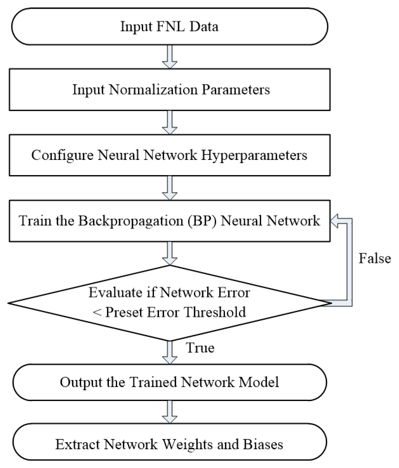
The BP algorithm was employed to train the neural network. To ensure both the retrieval accuracy and generalization capability of the model, ten years of reanalysis data were used for training. Given the large dataset, a simple cross-validation approach was adopted to effectively maintain model stability. During cross-validation, 90% of the data were used as the training set and the remaining 10% as the validation set. The model was trained solely on the training set and evaluated on the validation set to prevent overfitting and to optimize model parameters. Data from January, April, July, and October 2024 were used as the test set for final performance evaluation. The parameters used during training are summarized in Table 2 below:
The weights and biases of the network are determined by the error backpropagation algorithm during the training process. By continuously adjusting the network’s weights and biases, the deviation between the output vector calculated from the network’s input vector and the actual training target output vector is minimized. In the actual calculation of atmospheric profile retrieval, only its weight matrix and biases need to be invoked.
The specific implementation flow chart is described in Figure 2.

2.3. Accuracy Analysis Method

The accuracy of microwave radiometer modeling is commonly evaluated by the root Root Mean Square Error (RMSE). To assess the performance of the retrieval model developed in this study based on FNL reanalysis data, the retrieved temperature, water vapor density, relative humidity, and IWV were compared with observations from the Qingdao radiosonde station. In addition to the RMSE, Mean Absolute Error (MAE), Relative deviation, and Bias were also introduced as evaluation indicators, aiming to provide a comprehensive assessment of the retrieval performance from multiple perspectives.
The temperature profile, water vapor density profile, relative humidity profile, and IWV obtained by inputting parameters such as microwave radiometer brightness temperature, surface temperature, humidity, and pressure into the retrieval model are taken as test objects, which are compared with data from radiosonde data. RMSE, MAE, Bias and Relative Deviation (RD) are used as the bases for evaluating retrieval accuracy. The calculation formulas are as follows [34]:
R M S E = 1 n i = 1 n M o d i R a d i 2
M A E = 1 n i = 1 n M o d i R a d i
B i a s = 1 n i = 1 n M o d i R a d i
R D = 1 n i = 1 n M o d i R a d i R a d i
In the above formula, Modi represents the physical quantity output by the retrieval model, Radi represents the physical quantity obtained by the radiosonde data, n represents the total number of samples, and i represents the i-th sample.
To systematically evaluate the error distribution characteristics of the retrieval results with height and season, and to provide an analytical basis for subsequent targeted improvements, this study adopts error analysis based on multiple data classifications:
(1)
Vertical stratification diagnosis: Calculate the RMSE, MAE, and Bias of each height layer of the 83 layers layer by layer.
(2)
Seasonal assessment: For each independent month model (January, April, July, and October represent winter, spring, summer, and autumn), the error of the entire elevation layer from 0 to 10,000 m of all time periods in each month is statistically analyzed to quantify the seasonal variation characteristics.
(3)
Total performance test: Integrate the observation data of all time periods and all heights over four months, and calculate the comprehensive error index of all time periods and heights to evaluate the universality of the model.

3. Results and Analysis

3.1. Seasonal Analysis of Retrieval Results

For this analysis, retrieval results from the Qingdao region for 2024 were selected. To assessthe model’s adaptability across seasons [35,36], January, April, July, and October were chosen as representative months for winter, spring, summer, and autumn, respectively. The retrieval results of four months were compared with radiosonde data to validate the reliability of the neural network model established using reanalysis data in different seasons.

3.1.1. Analysis of Retrieval Results of Temperature

Figure 3 presents the comparison between the retrieved and observed temperature profiles for different months. The results show good temporal and spatial consistency with radiosonde data. In particular, the retrieval model successfully reproduces the inversion layers observed in April and October, indicating that the model outputs reliably capture the actual variability of atmospheric temperature.
Figure 4 displays the retrieved temperature profiles for each month. The smallest errors occur in July, while the largest errors are observed in April. Within the 0–2 km layer, errors increase rapidly, which can be attributed to near-surface inversion layers and the inherent detection characteristics of microwave radiometers. During summer, stronger surface convection reduces the likelihood of inversion layers, and the boundary layer height is generally higher, leading to more homogeneous low-level temperature distributions. As a result, the retrievals below 2 km perform best in July, with RMSE values within 1 °C. Above 2 km, retrieval errors gradually increase with altitude, reaching a maximum RMSE of 3.2 °C. Bias results further reveal notable negative deviations in April, July, and October at higher altitudes, with a maximum bias of −1.8 °C. In January, negative biases dominate below 5 km, while positive biases appear above 5 km, with the largest reaching 2.1 °C. Overall, the retrieval errors remain relatively small across all months, confirming the robustness of the proposed approach.
To eliminate discrepancies in data volume across altitude intervals caused by uneven vertical stratification, and to analyze the distribution of retrieval errors across different ranges, both the retrieved and radiosonde profiles were resampled at 100 m vertical intervals for comparison. As shown in Figure 5, the retrieval results exhibit good agreement with the observations. In January, the data show smaller dispersion at lower altitudes (temperature > −20 °C), while at higher altitudes with colder temperatures (temperature < −20 °C), the dispersion increases and the retrieval tends to overestimate the actual temperature. In July, the retrieval accuracy relative to radiosonde measurements is markedly improved compared with other seasons, yielding the smallest errors. In April and October, the correlation between retrievals and radiosonde data is strong, and the Bias distribution is approximately symmetric. Overall, the degree of dispersion increases with decreasing temperature, consistent with the vertical error distribution shown in Figure 4.

3.1.2. Analysis of Retrieval Results of Water Vapor Density

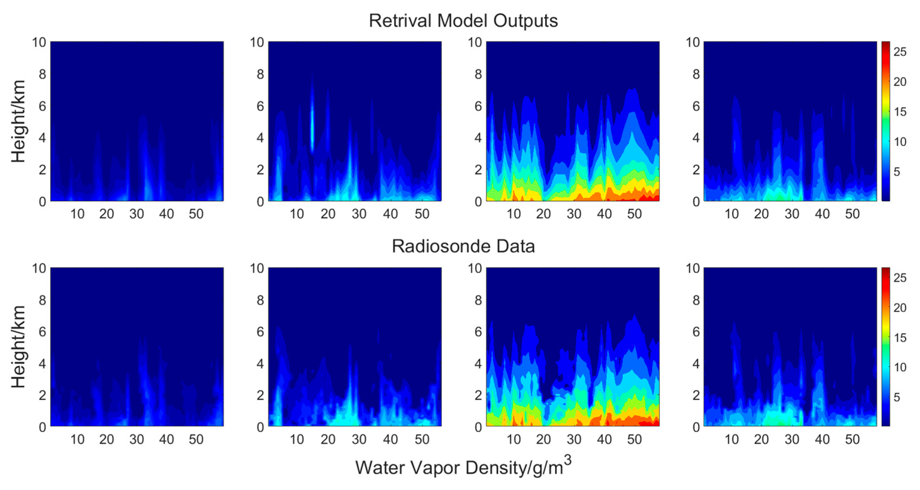
Figure 6 illustrates that the retrieved water vapor density profiles are generally consistent with radiosonde data. Water vapor density is highest within the 0–2 km layer and decreases rapidly with altitude, with both retrievals and observations showing similar vertical patterns.
Figure 7a–c present the absolute errors of water vapor density, while Figure 7d further shows the relative errors to avoid underestimating errors caused by the generally low water vapor content. From the distribution of absolute errors, it can be seen that January exhibits the smallest errors due to the limited water vapor, whereas April shows the largest absolute errors. However, as shown in Figure 7d, July has the smallest relative errors, while April shows the largest. The vertical distribution of relative errors follows a pattern similar to that of temperature errors: rapid growth below 2 km and slower growth above 2 km. Within the 0–2 km layer, retrievals exhibit a systematic negative bias, indicating an underestimation of water vapor, while above 2 km the bias becomes positive. Among all months, April shows the largest errors, with a maximum RMSE of 2.5 g/m3 and a maximum relative error of 0.9%. Overall, the retrieval performance is satisfactory.
Figure 8 shows that water vapor density is mainly concentrated within the 0–1 g/m3 range. However, in July, higher water vapor content is more frequent, leading to markedly better consistency in the high-density region (upper-left portion of the figure) compared with other months. Across the study region, July exhibits the best agreement between retrievals and radiosonde data, while January shows the worst, consistent with the seasonal distribution of absolute errors.

3.1.3. Analysis of Retrieval Results of Relative Humidity

As shown in Figure 9, relative humidity exhibits pronounced seasonal variations, with the highest values in July and the lowest in January. Because relative humidity is influenced by both temperature and water vapor density, its vertical structure is more complex. Nevertheless, the retrieved vertical distribution agrees well with the radiosonde data.
The seasonal variations in relative humidity exhibit generally consistent trends across all months. However, given its definition, relative humidity is jointly influenced by both water vapor density and temperature, leading to a more complex vertical variation pattern. The relative humidity errors display a bimodal distribution, with maxima at approximately 1 km and 5 km, consistent with the locations of maximum water vapor density errors. Yet, because temperature errors increase with altitude, the relative humidity errors above 5 km do not decrease as markedly as the water vapor density errors. In January, when water vapor content is lowest, the relative humidity errors above 5 km show some decrease with altitude, while in the other three months the errors remain nearly constant above 5 km. As shown in Figure 10c, the Bias distribution of relative humidity mirrors that of water vapor density, with negative biases in the lower atmosphere and positive biases at higher altitudes. The analysis indicates that water vapor density exhibits the highest retrieval accuracy in January, while relative humidity achieves its highest accuracy in July, which is related to the high accuracy of temperature in July. From a physical perspective, relative humidity is determined jointly by temperature and water vapor density. In July, the high precision of temperature makes a significant contribution to the accuracy of relative humidity. Although temperature and absolute humidity show relatively large errors in April, the relative humidity retrieval error for that month is not the worst among all months. This is because the temperature and absolute humidity errors partially compensate each other in the computation of relative humidity.
July exhibits the highest retrieval accuracy, with RMSE values below 24% at all altitudes.
Figure 11 shows that, due to the physical characteristics of relative humidity, its retrievals are less consistent with radiosonde data compared with temperature and water vapor density, although most values still cluster around the y = x line. In April, the climate is wetter than in winter, and the relative humidity values are mainly concentrated between 5–10% and 30–50%. Since the low relative humidity values in April are primarily located in the upper atmosphere, where retrieval accuracy is lower, the correlation in the 30–50% range is better than that in the 5–10% range. In July, radiosonde data are concentrated between 70–100%, but the retrieval results tend to underestimate these values.
Comparisons between retrievals and radiosonde data across different seasons indicate that retrievals perform well in all cases, accurately capturing the variations of atmospheric variables. Among them, July shows the smallest errors in both temperature and relative humidity retrievals. Although the absolute error of water vapor density is largest in July due to the higher water vapor content, the relative error remains smaller than in the other three months.

3.1.4. Analysis of Retrieval Results of IWV

The comparison and average deviation of IWV over the four months are shown in Figure 12. As seen in the figure, the overall consistency between the two datasets is very high. When IWV experiences a sharp increase or decrease, the patterns remain synchronous. The distribution of IWV errors in each season is consistent with the water vapor density error distribution. Notably, IWV reaches its annual peak in summer, approximately 40–80 mm. Overall, as a key instrument for IWV retrieve, the microwave radiometer has achieved satisfactory retrieval results for IWV.
From these results, it is evident that the retrieval results of the neural network model based on reanalysis data, are consistent with actual radiosonde data, and the trends in parameter variation across months show a marked degree of similarity.

3.2. The Statistical Result of Root Mean Square Error

Table 3 shows the error distribution of various atmospheric parameters across different seasons. As discussed in Section 3.1, the atmospheric parameters error retrieval characteristics vary significantly around 2 km. Therefore, the error statistics are divided into two categories: 0~2 km and >2 km.
As can be seen from Table 3, the total errors of temperature and relative humidity are relatively small below 2 km, while above 2 km, due to the increase in height, the total errors of the two increase significantly. The error is relatively large when the relative humidity is below 2 km. Due to the reduced water vapor content at high altitudes, the error above 2 km decreases. In both the upper and lower layers, the retrieval performance of temperature and relative humidity is the best in July. The retrieval performance of the entire layer temperature and the relative humidity of the upper layer in April is the worst, and the retrieval performance of relative humidity in the lower layer is the worst in January. Due to the lower water vapor content in January, the retrieval performance of water vapor density in the upper and lower layers is the best. The retrieval performance of water vapor density in the lower layer is the worst in July, and that in the upper layer is the worst in April. The retrieval performance of integral water vapor content is consistent with the law of water vapor density, with the best in January and the worst in July.
Overall, the retrieval performance of temperature and relative humidity at the lower layer is better than that at the upper layer, but the retrieval performance of water vapor density at the lower layer is worse than that at the upper layer. On average across the entire layer, the retrieval performance of temperature is the worst in January, the retrieval performance of temperature and relative humidity is the best in July, and the retrieval performance of water vapor density is the best and that of temperature is the worst in January. There are significant seasonal differences in high layer temperature errors. The temperature of the high layer is overestimated in winter and underestimated in the other three seasons. The water vapor density and relative humidity in each season are both underestimated at the lower layer and at the upper layer. The retrieval accuracy of the model was relatively high.

4. Conclusions

In this paper, a microwave radiometer retrieval algorithm based on FNL reanalysis data was developed to obtain atmospheric temperature profiles, water vapor density profiles, relative humidity profiles, and IWV. These retrievals were compared with synchronous radiosonde data, and the following conclusions were drawn:
(1)
The vertical error distribution indicates that temperature and humidity errors increase with altitude in each season. The error in water vapor density increases rapidly from the surface to 1 km, then gradually decreases. Temperature and relative humidity errors increase most rapidly below 2 km.
(2)
The retrieval performance of different meteorological variables exhibits seasonal variations. The retrieval accuracy of temperature profiles is highest in summer and lowest in spring. The relative humidity profile also performs best in summer and worst in winter. However, the retrieval accuracy of water vapor density profiles and IWV is best in winter and worst in summer. This is due to enhanced radiation scattering by large water droplets in the summer atmosphere, which introduces measurement errors in brightness temperature. Additionally, large variations in the humidity field complicate the retrieval process. In winter and spring, low-level inversions are more prominent, with substantial variations in the thickness and intensity of the inversion layer, making it challenging to retrieve refined temperature profiles.
(3)
The results of the neural network retrieval based on FNL reanalysis data are generally consistent with the radiosonde data. The comprehensive statistics of the entire layer show that in the near surface layer (0–2 km) and mid-upper layer (>2 km), the RMSE of the temperature profile retrieve results are 1.15 °C and 2.05 °C respectively, and the RMSE of the relative humidity are 14.01% and 20.79% respectively. The RMSE of water vapor densities are 1.25 g/m3 and 0.62 g/m3 respectively and RMSE of IWV is 1.37 mm. Overall, the retrieval results exhibit small errors, demonstrating that this method is reliable and practical for atmosphere observing.
Reference [23] compared a microwave radiometer neural network model based on ERA5 reanalysis data with radiosonde data. The MAE of temperature, water vapor density, and relative humidity profiles retrieved from ERA5 relative to radiosonde data were 2.402 °C, 0.412 g/m3, and 15.587%, respectively, while the corresponding RMSE were 2.748 °C, 0.575 g/m3, and 16.864%. In this study, the temperature retrieval results based on FNL data outperform those from ERA5, whereas the water vapor density and relative humidity retrievals are slightly lower than the ERA5-based results. The research findings indicate that the retrieval results from the microwave radiometer model constructed with FNL data are generally consistent with radiosonde data, with retrieval errors falling within an acceptable range. This suggests that using reanalysis data for the construction of retrieval models is feasible. However, our analysis is limited to the Qingdao region, and the applicability of the results to other regions has not yet been addressed. Given the broad spatial coverage of reanalysis datasets, the modeling approach proposed demonstrates high portability. However, for different regions, the model must be retrained by using the reanalysis data specific to nearby stations to construct region-specific retrieval models. Additionally, a comprehensive evaluation of the retrieval performance, in combination with other reanalysis data, is necessary to provide effective guidance for microwave radiometer observations in areas lacking radiosonde data. Future work should focus on more in-depth research into the limitations, potential biases, and regional applicability of different reanalysis data.

Author Contributions

Conceptualization, Q.Z.; methodology, X.L.; validation, X.L.; formal analysis, X.D.; resources, H.C.; data curation, T.S.; writing—original draft preparation, X.L.; writing—review and editing, W.W.; visualization, X.L. and W.W.; supervision, Q.Z.; project administration, X.D.; funding acquisition, Q.Z. and B.X. All authors have read and agreed to the published version of the manuscript.

Funding

This research was funded by the National Natural Science Foundation of China (Grant No. 62201529), Shandong Provincial Natural Science Foundation (No. ZR2024QD072) and Stable-Support Scientifit Project of China Research of Radiowave Propagation (A240204150).

Institutional Review Board Statement

Not applicable.

Informed Consent Statement

Not applicable.

Data Availability Statement

The data used in this study are available upon request from the corresponding author due to privacy restrictions.

Acknowledgments

Thanks to the editor and all reviewers for their valuable comments.

Conflicts of Interest

The authors declare no conflicts of interest.

Abbreviations

The following abbreviations are used in this manuscript:
BPBack Propagation
ERA5ECMWF Reanalysis 5th Generation
FNLFinal Reanalysis
GDASGlobal Data Assimilation System
IWVIntegrated Water Vapor
LSTMLong Short Term Memory
MAEMean Absolute Error
NCEPNational Centers for Environmental Prediction
RBFRadial Basis Function
RDRelative Deviation
RMSERoot Mean Square Error

References

  1. Ware, R.H.; Solheim, F.S. Microwave profiling of atmospheric temperature, humidity, and cloud liquid water. Mirow. Remote Sens. Atmos. Environ. 2000, 4152, 292–302. [Google Scholar]
  2. Zhang, X.F.; Wang, Z.C.; Mao, J.J.; Wang, Z.W.; Zhang, D.M.; Tao, F. Experiments on improving temperature and humidity profile retrieval for ground-based microwave radiometer. J. Appl. Meteorol. Sci. 2020, 31, 385–396. (In Chinese) [Google Scholar]
  3. Zhang, W.G.; Xu, G.R.; Yan, G.P.; Li, N.; Huang, Z.Y.; Feng, G.L. Comparative analysis of microwave radiometer and radiosonde data. Meteorol. Sci. Technol. 2014, 42, 737–741. (In Chinese) [Google Scholar]
  4. Yuan, S.; Cheng, H.; Wang, D.Y.; Zhou, J. Comparative analysis on meteorological parameters of sounding data and model-generated sounding data. J. Meteorol. Sci. 2012, 32, 62–67. (In Chinese) [Google Scholar]
  5. Lei, L.F.; Lu, J.P.; Zhu, L.; Wu, H. Atmospheric remote sensing using multi-channel ground-based microwave radiometer. J. Remote Sens. 2014, 18, 180–191. (In Chinese) [Google Scholar] [CrossRef]
  6. Churnside, J.H.; Stermitz, T.A.; Schroeder, J.A. Temperature profiling with neural network inversion of microwave radiometer data. J. Atmos. Ocean. Technol. 1994, 11, 105–109. [Google Scholar] [CrossRef]
  7. Smith, W.L.; Woolf, H.M. The use of eigenvectors of statistical covariance matrices for interpreting satellite sounding radiometer observations. J. Atmos. Sci. 1976, 33, 1127–1140. [Google Scholar] [CrossRef]
  8. Li, Z.; Li, J.; Menzel, W.P.; Nelson, J.P., III; Schmit, T.J.; Weisz, E.; Ackerman, S.A. Forecasting and nowcasting improvement in cloudy regions with high temporal GOES sounder infrared radiance measurements. J. Geophys. Res. Atmos. 2009, 114, D09216. [Google Scholar] [CrossRef]
  9. Cao, X.F.; Li, X.Y.; Luo, Q.; Liu, S.H.; Li, P.; Liu, X. Review of temperature profile inversion of satellite-borne infrared hyperspectral sensors. Natl. Remote Sens. Bull. 2021, 25, 577–598. (In Chinese) [Google Scholar]
  10. Cadeddu, M.P.; Turner, D.D.; Liljegren, J. A neural network for real-time retrievals of PWV and LWP from Arctic millimeter-wave ground-based observations. IEEE Trans. Geosci. Remote 2009, 47, 1887–1900. [Google Scholar] [CrossRef]
  11. Solheim, F.; Godwin, J.R.; Westwater, E.R.; Han, Y.; Keihm, S.J.; Marsh, K.; Ware, R. Radiometric profiling of temperature, water vapor and cloud liquid water using various inversion methods. Radio Sci. 1998, 33, 393–404. [Google Scholar] [CrossRef]
  12. Fan, X.; Huang, Y.; Leng, W.N.; Zhang, B.D.; Zhang, W.Y. Inversion of ground-based microwave radiometer measurements using radial basis function neural network. J. Meteorol. Environ. 2020, 36, 62–69. (In Chinese) [Google Scholar]
  13. Zhou, G.J.; Yang, Z.P.; Peng, J.; Yang, L.; Tao, F.; Mao, J.J. Humidity Profile Inversion of Ground Based Microwave Radiometer Based on LSTM. Meteorol. Sci. Technol. 2022, 50, 21–29. [Google Scholar] [CrossRef]
  14. Liu, Y.Y.; Mao, J.T.; Liu, J.; Li, F. Research of BP neural network for microwave radiometer remote sensing retrieval of temperature, relative humidity, cloud liquid water profiles. Plateau Meteorol. 2010, 29, 1514–1523. (In Chinese) [Google Scholar]
  15. Yang, M.Y. Research on Atmospheric Parameter Retrieval Method Based on Ground-Based Microwave Radiometer. Master’s Thesis, Nanjing University of Science &Technology, Nanjing, China, 2023. [Google Scholar]
  16. Huang, X.Y.; Zhang, X.; Leng, L.; Li, F.; Fan, Y.W. Study on retrieval methods with MonoRTM for microwave radiometer measurements. Meteorol. Sci. Technol. 2013, 33, 138–145. (In Chinese) [Google Scholar]
  17. Valjarević, A.; Filipović, D.; Valjarević, D.C.; Milanović, M.; Milošević, S.; Živić, N.; Lukić, T. GIS and remote sensing techniques for the estimation of dew volume in the Republic of Serbia. Meteorol. Appl. 2020, 27, e1930. [Google Scholar] [CrossRef]
  18. Zhao, T.B.; Fu, C.B.; Ke, Z.J.; Guo, W.D. Global atmosphere reanalysis datasets: Current status and recent advances. Adv. Earth Sci. 2010, 25, 241–254. (In Chinese) [Google Scholar]
  19. Hersbach, H.; Bell, B.; Berrisford, P.; Hirahara, S.; Horányi, A.; Muñoz-Sabater, J.; Nicolas, J.; Peubey, C.; Radu, R.; Schepers, D.; et al. The ERA5 global reanalysis. Q. J. R. Meteorol. Soc. 2020, 146, 1999–2049. [Google Scholar] [CrossRef]
  20. Hayes, L.; Stocks, M.; Blakers, A. Accurate long-term power generation model for offshore wind farms in Europe using ERA5 reanalysis. Energy 2021, 229, 120603. [Google Scholar] [CrossRef]
  21. Gleixner, S.; Demissie, T.; Diro, G.T. Did ERA5 Improve temperature and precipitation reanalysis over East Africa? Atmosphere 2020, 11, 996. [Google Scholar] [CrossRef]
  22. Carvalho, D.; Rocha, A.; Gómez, G.M.; Silva, S.C. Comparison of reanalyzed, analyzed, satellite-retrieved and NWP modelled winds with buoy data along the Iberian Peninsula coast. Remote Sens. Environ. Interdiscip. J. 2014, 152, 480–492. [Google Scholar] [CrossRef]
  23. Hu, L.H.; Jiang, H.L.; Wang, H. Prelimiary application of ERA5 reanalysis data to retrieval method of microwave radiometer. Meteorol. Sci. Technol. 2023, 52, 163–172. [Google Scholar]
  24. Mangsuer, A.; Xiao, J.; Sun, M.; Yang, H. Comparative analysis on the applicability of ERA5 and FNL data in Xinjiang. Plateau Mt. Meteorol. Res. 2024, 44, 142–150. [Google Scholar]
  25. Zhang, Y.; Chen, J.H.; Tang, B.Y. Numerical simulation of meteorological elements of a pollution episode in Sichuan Basin based on two reanalysis datasets. Acta Sci. Circum. 2020, 40, 3093–3102. [Google Scholar]
  26. Li, Q.; Wei, M.; Wang, Z.; Chu, Y.; Ma, L. Evaluation and correction of ground-based microwave radiometer observations based on NCEP-FNL data. Atmos. Clim. Sci. 2019, 9, 229–242. [Google Scholar] [CrossRef]
  27. Wang, Z.C.; Zhang, X.F.; Mao, J.J.; Wang, Z.C. Comparison analysis on detection performance of ground-based microwave radiometers under different weather conditions. J. Appl. Meteorol. Sci. 2018, 29, 282–295. (In Chinese) [Google Scholar]
  28. De Angelis, F.D.; Cimini, D.; Löhnert, U.; Caumont, O.; Haefele, A.; Pospichal, B.; Martinet, P.; Navas-Guzmán, F.; Klein-Baltink, H.; Dupont, J.C.; et al. Long-term observation minus background monitoring of ground-based brightness temperatures from a microwave radiometer network. Atmos. Meas. Tech. 2017, 10, 3947–3961. [Google Scholar] [CrossRef]
  29. Zhou, X.J. Atmospheric Microwave Radiation and Remote Sensing Principle; Science Press: Beijing, China, 1983; 178p. (In Chinese) [Google Scholar]
  30. Navas-Guzmán, F.; Kämpfer, N.; Haefele, A. Validation of brightness and physical temperature from two scanning microwave radiometers in the 60GHz O2 band using radiosonde measurements. Atmos. Meas. Tech. 2016, 9, 4587–4600. [Google Scholar] [CrossRef]
  31. Clough, S.A.; Iacono, M.J.; Moncet, J.L. Line-by-line calculations of atmospheric fluxes and cooling rates: Application to water vapor. J. Geophys. Res. Atmos. 1992, 97, 15761–15785. [Google Scholar] [CrossRef]
  32. Clough, S.A.; Iacono, M.J. Line-by-line calculation of atmospheric fluxes and cooling rates: 2. Application to carbon dioxide, ozone, methane, nitrous oxide and the halocarbons. J. Geophys. Res. Atmos. 1995, 100, 16519–16535. [Google Scholar] [CrossRef]
  33. Egorov, D.P.; Verina, Y.V.; Kravchenko, O.V. Development of neural network approach for reconstructing the atmospheric humidity profile form ground-based microwave radiometer-spectrometer data. In Proceedings of the Photonics & Electromagnetics Research Symposium (PIERS), Chengdu, China, 21–25 April 2024. [Google Scholar] [CrossRef]
  34. Cao, M.; Wang, B.; Yang, Z.; Zhang, Y.M. Data comparison between ground-based microwave radiometer and radiosonde. J. Shaanxi Meteorol. 2021, 5, 47–54. (In Chinese) [Google Scholar]
  35. Bedoya-Velásquez, A.E.; Navas-Guzmán, F.; de Arruda Moreira, G.; Román, R.; Cazorla, A.; Ortiz-Amezcua, P.; Benavent-Oltra, J.A.; Alados-Arboledas, L.; Olmo-Reyes, F.J.; Foyo-Moreno, I.; et al. Seasonal analysis of the atmosphere during five years by using microwave radiometry over a mid-latitude site. Atmos. Res. 2019, 218, 78–89. [Google Scholar] [CrossRef]
  36. Renju, R.; Suresh Raju, C.; Mishra, M.K.; Mathew, N.; Rajeev, K.; Moorthy, K.K. Atmospheric boundary layer characterization using multiyear ground-based microwave radiometric observations over a tropical coastal station. IEEE Trans. Geosci. Remote Sens. 2017, 55, 6877–6882. [Google Scholar] [CrossRef]
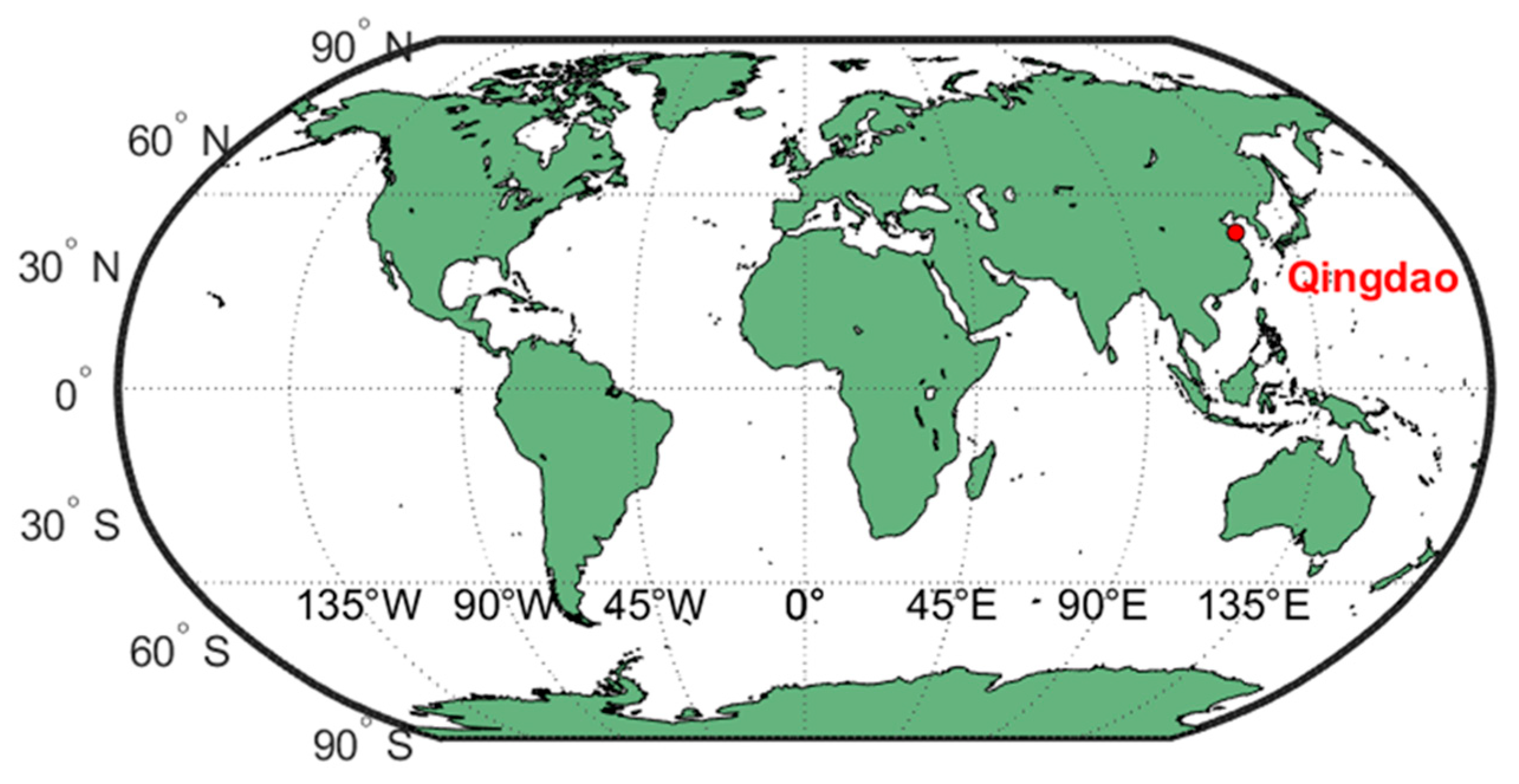
Figure 1. Location of Qingdao on the world map.
Atmosphere 16 01194 g001
Figure 2. The process of neural network training.
Atmosphere 16 01194 g002
Figure 3. Spatiotemporal distribution of retrieved temperatures and radiosonde data (first row: retrieval results; second row: radiosonde data; from left to right: January, April, July, October. The x-axis represents the sample sequence, and the y-axis represents altitude).
Atmosphere 16 01194 g003
Figure 4. Vertical distribution of temperature profile errors for each month: (a) RMSE, (b) MAE, (c) Bias. (Blue: January; Red: April; Yellow: July; Purple: October).
Atmosphere 16 01194 g004
Figure 5. Scatter plots of retrieved temperatures versus radiosonde data ((ad) correspond to January, April, July, and October, respectively; color shading represents the number of samples, and the black line indicates y = x).
Atmosphere 16 01194 g005
Figure 6. Spatiotemporal distribution of retrieved water vapor density and radiosonde data (first row: retrieval results; second row: radiosonde data; from left to right: January, April, July, October. The x-axis represents the sample sequence, and the y-axis represents altitude).
Atmosphere 16 01194 g006
Figure 7. Vertical distribution of water vapor density profile errors for each month: (a) RMSE, (b) MAE, (c) Bias, (d) Relative Deviation. (Blue: January; Red: April; Yellow: July; Purple: October).
Atmosphere 16 01194 g007
Figure 8. Scatter plots of retrieved water vapor density versus radiosonde data ((ad) correspond to January, April, July, and October, respectively; color shading represents the number of samples, and the black line indicates y = x).
Atmosphere 16 01194 g008
Figure 9. Spatiotemporal distribution of retrieved relative humidity and radiosonde data (first row: retrieval results; second row: radiosonde data; from left to right: January, April, July, October. The x-axis represents the sample sequence, and the y-axis represents altitude).
Atmosphere 16 01194 g009
Figure 10. Vertical distribution of relative humidity profile errors for each month: (a) RMSE, (b) MAE, (c) Bias. (Blue: January; Red: April; Yellow: July; Purple: October).
Atmosphere 16 01194 g010
Figure 11. Scatter plots of retrieved relative humidity versus radiosonde data ((ad) correspond to January, April, July, and October, respectively; color shading represents the number of samples, and the black line indicates y = x).
Atmosphere 16 01194 g011
Figure 12. IWV of different samples ((ad) represent January, April, July, and October, respectively). The blue solid line represents the retrieval result, the red solid line represents the radiosonde data, and the black dashed line represents the average deviation between the retrieval result and the radiosonde data.
Atmosphere 16 01194 g012
Table 1. Performance parameters of QWF-6000 microwave radiometer.
EquipmentQFW-6000
Parameters
Detection range0~10 km
Technical systemMixing frequency detection
Brightness temperature sensitivityWater vapor channel ≤0.2 K (1 s integration)
Oxygen channel ≤0.3 K (1 s integration)
Measurement error of bright temperature≤1 K (RMS)
Observe the bright temperature range0~400 K
Frequency range and number of channels22~32 GHz: 8 vapor channels
52~59 GHz: 8 temperature channels
Long-term stability of bright temperature≤0.1 K/month
Sampling frequency≤2 min(Fastest 10 s)
Observation modezenith observation
Table 2. Training parameters for the BP neural network retrieval model.
Parameter TypeValue
The number of neurons in the input layer20
The number of neurons in the hidden layer41
The number of neurons in the output layer83
The number of training samples13,140
The number of validation samples1460
The number of test samples213
Maximum number of iterations5000
Table 3. Error statistics (RMSE, MAE, Bias) of the retrieval results of atmospheric parameters.
MonthJanuaryAprilJulyOctoberTotal
Error
Variable
Temperature (°C)
(0~2 km)
RMSE1.071.340.951.201.15
MAE0.650.810.570.720.69
Bias−0.0440.005−0.0005−0.036−0.02
Temperature (°C)
(>2 km)
RMSE2.092.341.512.262.05
MAE1.802.061.251.881.75
Bias0.76−1.41−0.56−0.83−0.51
Water vapor density
(0~2 km)
RMSE0.611.571.611.211.25
MAE0.441.191.150.980.94
Bias−0.13−0.68−0.40−0.53−0.44
Water vapor density
(>2 km)
RMSE0.261.020.750.460.62
MAE0.150.460.560.320.37
Bias0.060.300.150.150.16
Relative humidity
(0~2 km)
RMSE17.6515.449.9913.0614.01
MAE12.5912.287.4710.7510.77
Bias−5.37−5.96−2.23−4.17−4.43
Relative humidity
(>2 km)
RMSE20.8722.0518.6421.4920.79
MAE15.9617.5114.6317.0316.28
Bias10.197.132.496.506.58
IWVRMSE0.651.312.161.201.37
MAE0.430.891.590.910.95
Bias0.090.130.190.160.14
Disclaimer/Publisher’s Note: The statements, opinions and data contained in all publications are solely those of the individual author(s) and contributor(s) and not of MDPI and/or the editor(s). MDPI and/or the editor(s) disclaim responsibility for any injury to people or property resulting from any ideas, methods, instructions or products referred to in the content.