The Characteristics and Possible Mechanisms of the Strongest Ionospheric Irregularities in March 2024

Abstract

A geomagnetic storm occurred on 3 March 2024, with the minimum SYM-H reaching −127 nT. Although this geomagnetic storm was not very strong, the ionospheric irregularities on this day resulted in a strong ionospheric scintillation. The amplitude scintillation index was larger than 1.0. Global Navigation Satellite System (GNSS) receivers experienced numerous cycle slips and loss of lock of carrier phase over a large longitudinal range of ~30 degrees within ~5 h in the south of China. The occurrence of cycle slips over such a long duration and extensive longitudinal range is rarely reported. Ground-based GNSS receivers, ionosondes and in situ satellite measurements were utilized to analyze the characteristics of the equatorial plasma bubbles (EPBs) during this event. The EPBs began before the main phase of the geomagnetic storm and extended to 30°N in latitude. Possible physical mechanisms for the initial generation and the development of the EPBs are discussed. It is believed that different mechanisms played vital roles in the initial generation and development of the EPBs before and after the onset of the main phase of the geomagnetic storm. Moreover, a large-scale wave structure (LSWS) could potentially serve as the seeding source of the EPBs.

1. Introduction

Ionospheric irregularities have been studied for about 50 years. According to their effect on detection equipment, they are called spread F (SF) in ionograms [1], ionospheric scintillation [2], plumelike structures in radar maps [3] and plasma bubbles in in situ electron density measurements [4]. The irregularities have significant impacts on radio wave propagation and communication and navigation systems; they even cause outages of radio systems [5]. Global Navigation Satellite System (GNSS) receivers will undergo cycle slips or loss of lock on the carrier phase if scintillation is severe enough [6]. The temporal dependence of GNSS cycle slip is related to ionospheric irregularities over China’s low-latitude region [7,8]. Therefore, it is important to study the characteristics and the evolution of the irregularities.

Equatorial plasma bubbles (EPBs) are plasma density depletion structures that occur near the magnetic equator. They generally develop after sunset under the generalized Rayleigh–Taylor (R-T) instability [5]. After sunset, the bottom of the F layer becomes unstable because of the large vertical gradient of electron density. When a perturbation occurs at the bottom of the F layer, the pre-reversal enhancement (PRE) of the eastward electric field will uplift the F layer and magnify the perturbation, forming the typical post-sunset EPBs [9]. The large-scale wave-like structure (LSWS) in the bottom side of the F layer is thought to be one of the seeding sources of EPBs [10]. Post-sunset EPBs more commonly occur in equinox months during high solar activity years in the East and Southeast Asian sector because the angle between the magnetic field lines and the sunset terminator is small in equinoctial months [11,12,13].

During geomagnetic storms, the ionosphere, electric field, neutral wind and neutral atmosphere become disturbed and complex. The EPBs may also show different characteristics from those on quiet days. In some cases, EPBs are enhanced while in some other cases they are inhibited [14]. When they are enhanced, they can extend to mid-latitudes [15,16] or cover a wide longitudinal range [17]. In contrast, EPBs are sometimes suppressed or confined within a narrow longitudinal range [18,19].

The prompt penetration electric field (PPEF) associated with the interplanetary magnetic field (IMF) Bz turning southward or northward can penetrate from high latitudes to low latitudes and thereby affect the generation and development of EPBs [20]. The disturbance dynamo electric field (DDEF) due to storm-time neutral wind [21] and storm-time equatorward neutral winds may also become an additional driver of EPBs [22]. The direction of PPEF, DDEF, storm-time neutral wind and the competing mechanism depend on the onset time of the geomagnetic storm; therefore, the occurrence of EPBs is complicated and unpredictable during geomagnetic storms, showing enhancement or inhibition. Although lots of studies have been conducted on storm-time EPBs, the characteristics, seeding sources and development of the EPBs are still unclear, and how the PPEF and other factors affect the EPBs, especially during moderate geomagnetic storms [23].

March 2024 is equinox time and overlaps with a high solar activity year, providing suitable conditions for the occurrence of EPBs. During this month, ionospheric scintillation was observed on 25 days in Fuke (19.53° N, 109.13° E), Hainan. The strongest scintillation in this month occurred on 3 March 2024, and this was reported by the Space Environment Prediction Center, National Space Science Center, Chinese Academy of Sciences, on the website http://www.sepc.ac.cn (accessed on 10 July 2024). On 3 March 2024, a moderate geomagnetic storm occurred with a minimum SYM-H reaching −127 nT. The strongest ionospheric scintillation on this day might be related to the geomagnetic storm.

In this paper, we focus on the characteristics and evolutions of EPBs, analyze the impact of the geomagnetic storm on EPBs, and discuss the possible physical mechanisms and seeding sources. This paper is arranged as follows. In Section 2, the data and method are given. The results from multi-instruments are shown in Section 3. A discussion of the characteristics and possible mechanisms is provided in Section 4. Finally, the conclusions are summarized in Section 5.

2. Data and Methods

The IMF-Bz, ASY-H and SYM-H data with a 5 min resolution were downloaded from the OMNI database and used to examine the IMF magnetic field and geomagnetic conditions during this event.

Ground-based GNSS total electron content (TEC) and scintillation measurements were used to show the characteristics of the ionospheric irregularities during the geomagnetic storm. Figure 1 shows the GNSS Ionospheric Observation Network (GION) in the southern part of China established by the National Astronomical Observatories of Chinese Academy of Sciences (NAOC). The black dots represent the GNSS dual-frequency receivers sampling the pseudorange and carrier phase at a rate of 1 Hz. The star indicates the location of the GNSS scintillation receiver that samples at 50 Hz.

Six ionosondes established by the Meridian Space Weather Monitoring Project (Meridian Project for short), the Global Ionosphere Radio Observatory (GIRO), the National Institute of Information and Communications Technology (NICT) of Japan and the Southeast Asia Low-latitude IOnospheric Network (SEALION) were utilized to detect the spread traces and ionospheric variations on 3 March 2024. Their locations are listed in

Table 1. Locations of the ionosondes.

Station ID	Geographic Latitude (°N)	Geographic Longitude (°E)	Geomagnetic Latitude (°N)	Organization
IC437	37.14	127.54	31.49	GIRO
Wuhan	30.50	114.48	22.45	Meridian Project
OKI	26.68	128.15	18.55	NICT
Fuke	19.53	109.13	14.08	Meridian Project
CMU	18.76	98.93	9.33	SEALION
CPN	10.72	99.37	1.33	SEALION

.

The in situ measurements from FORMASAT-5 and SWARM-C were also utilized to analyze the irregularities together with the ground-based instruments. FORMASAT-5 operates in a sun-synchronous orbit with an inclination of 98.28° at an altitude of 720 km, traversing the 10:30/22:30 local time (LT) sector [24]. SWARM-C detects plasma density at a height of ~470 km above the ground [25].

The GNSS receivers of GION sample the dual-frequency pseudorange and phase of GPS, BDS and Galileo at 1 Hz. A mask angle of 30° is applied to reduce the effect of multipath. The line-of-sight TEC (slant TEC, short for sTEC) can be obtained from the dual-frequency measurement. With the single thin shell ionosphere at the height of 400 km, the vertical TEC (vTEC) at the ionosphere piercing points (IPPs) is obtained by multiplying sTEC by the cosine of the zenith angle at the IPPs. And then the rate of TEC change (ROT) is taken from the time derivative of vTEC with 30 s sampling intervals, and the rate of TEC index (ROTI), defined by $\mathrm{R}\mathrm{O}\mathrm{T}\mathrm{I}=\sqrt{〈{\mathrm{R}\mathrm{O}\mathrm{T}}^2〉-{〈\mathrm{R}\mathrm{O}\mathrm{T}〉}^2}$, is computed with a 5 min time running window [26]. A threshold of ROTI > 0.2 TECU/min is set to identify EPBs.

For BDS-GEO, temporal fluctuation in TEC (TFT) is used to detect EPBs because of the fixed IPPs. TFT is defined as the standard deviation of vTEC [27].

$$\mathrm{T}\mathrm{F}\mathrm{T}=\sqrt{〈{\mathrm{v}\mathrm{T}\mathrm{E}\mathrm{C}}^2〉-{〈\mathrm{v}\mathrm{T}\mathrm{E}\mathrm{C}〉}^2}$$

The Septentrio PolaRx5 ionospheric scintillation receiver at Xiamen (24.5° N, 118.0° E) can receive all of the signals from the GNSS. The amplitude scintillation index S₄ and 60 s phase scintillation index ${\mathsf{\sigma }}_{\mathsf{\phi }}$ are used to characterize the irregularities. S₄ based on BDS-GEO measurements is used to analyze the evolution of the EPBs.

3. Results

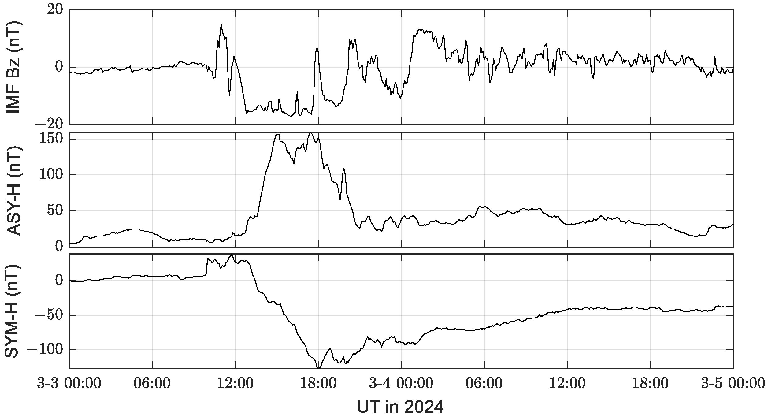
3.1. IMF and Geomagnetic Conditions

On 3 March 2024, a moderate geomagnetic storm occurred. IMF-Bz, ASY-H and SYM-H on 3–4 March 2024 are shown in Figure 2. Before the IMF-Bz turned southward, it increased suddenly during 10:35–11:00 UT. And then it decreased quickly and turned southward and reached a minimum of −16.07 nT at 12:50 Universal Time (UT). The IMF-Bz kept southward until 17:45 UT. From 17:45 to 23:55 UT, IMF-Bz oscillated between southward and northward directions.

Correspondingly, the SYM-H decreased rapidly from 12:50 UT, inferring the beginning of the main phase of the geomagnetic storm. It reached the minimum of −127 nT at 18:05 UT on 3 March. And then the geomagnetic storm went into the recovery phase, and SYM-H began to rise slowly.

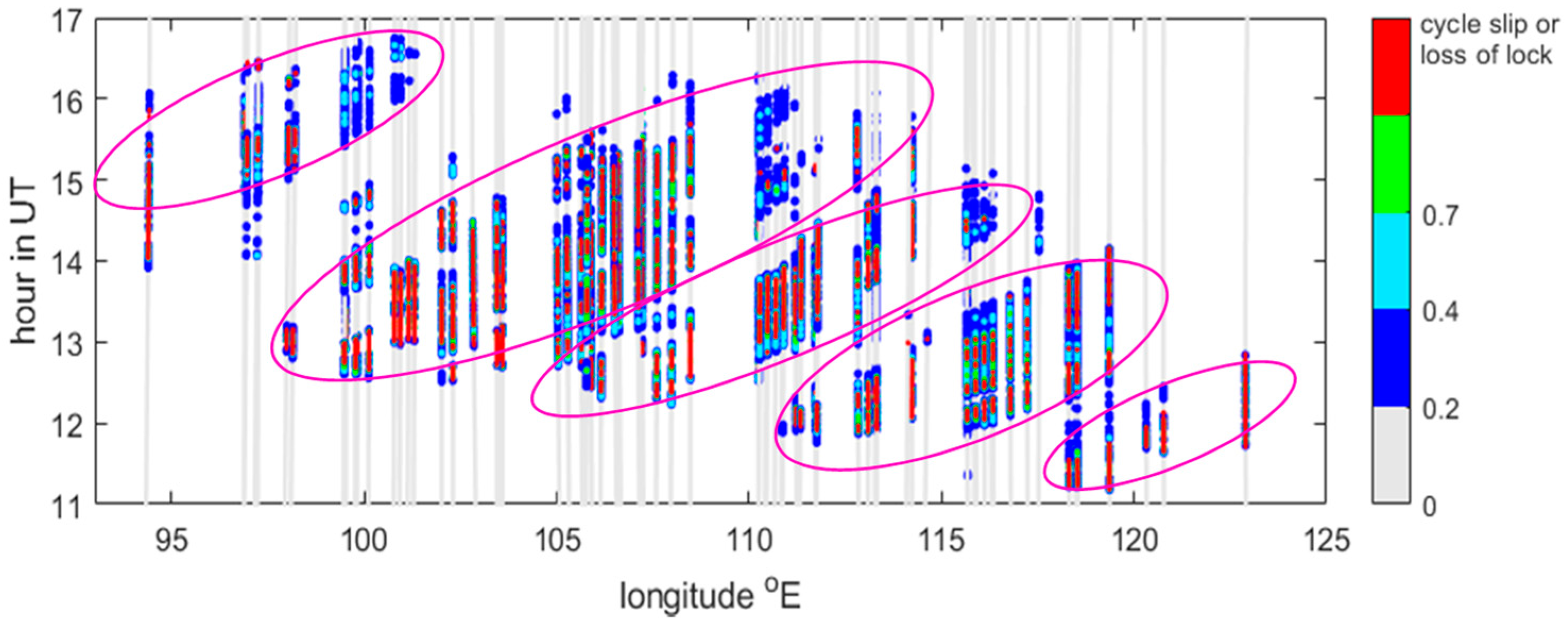
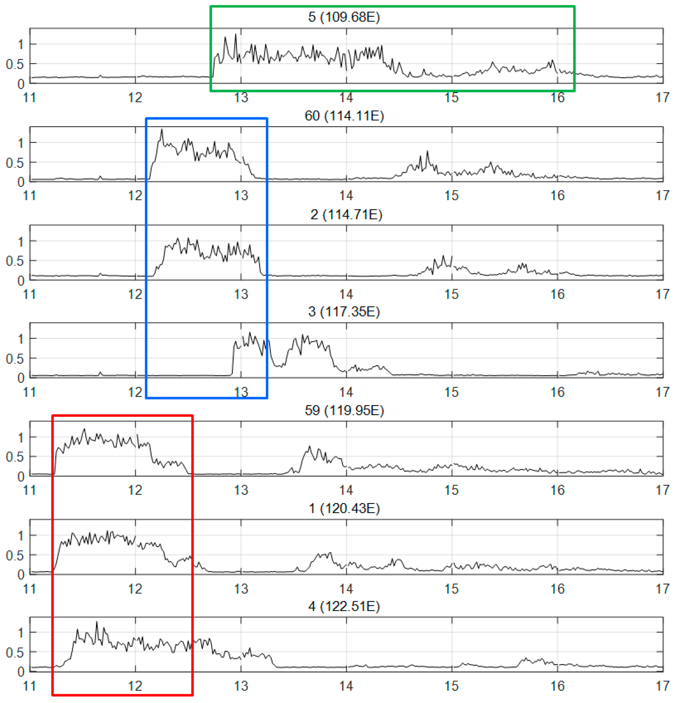
3.2. Results from BDS-GEO TFT

Figure 3 presents the BDS-GEO TFT (denoted as TFTg) keogram from the GION by the NAOC on 3 March 2024. The horizontal axis is the longitude, and the vertical axis is the UT in hours. The values of TFTg are presented by different colors as shown by the colorbar. The time window for acquiring TFTg was set to 30 s and the threshold to detect the EPBs is set to 0.2. If loss of lock or phase cycle slip occurs in any of the dual-frequency phase measurements within a 30 s period, it is impossible to calculate the sTEC/vTEC, or the calculated sTEC/vTEC is not reliable. Therefore, we did not calculate TFTg and marked the corresponding locations with red dots in the TFTg keogram, and labeled them as “cycle slip or loss of lock”.

Figure 3 shows the EPBs detected by the TFTg on 3 March 2024. The EPBs occurred after sunset at ~11:15 UT and survived until ~16:40 UT. They covered about 30° in longitude, spanning from 95 to 125° E. The earliest appearance of EPBs was observed at ~11:15 UT near the longitude of ~118° E. The EPBs survived for several hours before disappearing at ~16:40 UT. The EPBs were composed of five patches, which are circled by the magenta ellipses in Figure 3. Each of these patches drifted eastward, and the drift velocity ranged from ~150 m/s (for the two easternmost patches) to ~100 m/s (for the westernmost patch). The EPBs appeared successively following the progression of sunset from east to west. Moreover, the occurrences of the EPBs at a single IPP, represented by one vertical line in Figure 3, were intermittent.

The EPBs resulted in numerous cycle slips or losses of lock of the carrier phase, as shown by the red dots in the figure. The areas affected by the cycle slip or loss of lock spanned a large longitudinal range and persisted for several hours.

In the case of the three western patches, the occurrence of cycle slips or losses of lock gradually declined as the EPBs drifted eastward. Before the EPBs vanished, the values of TFTg weakened, and the phenomena of cycle slip and loss of lock almost disappeared.

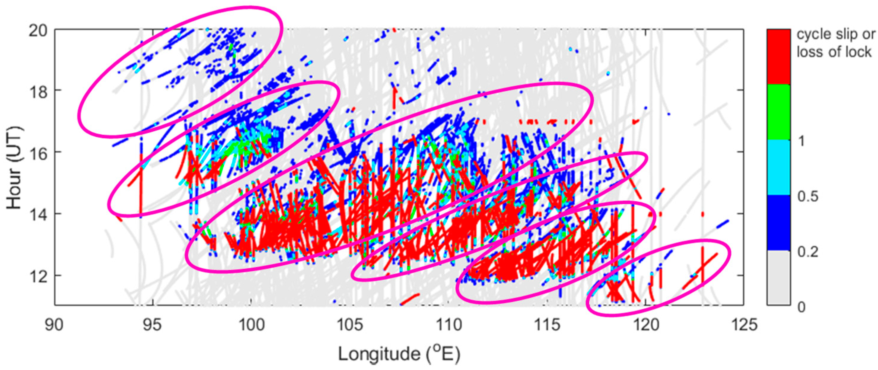
3.3. Results from ROTI

Figure 4 shows the ROTI keogram from the GION by the NAOC on 3 March 2024. The ROTIs were derived from the measurements of GPS, BDS and Galileo, with a sampling interval of 30 s. The red dots in the keogram represent ROTI data gaps. The gaps result from loss of lock or phase cycle slips within a 5 min period, and are labeled as “cycle slip or loss of lock” on the colorbar. The 30 s ROTI keogram detected six irregular patches, which are circled by the magenta ovals. After 17:00 UT, a new patch appeared at the top-left corner of the keogram, and this patch was not detected by the TFTg keogram. All of these patches drifted eastward during their evolution, similar to the TFTg observations. The four eastern patches caused more cycle slips or losses of lock than the two western patches. The irregularities detected by the ROTI keograms persisted until 20:00 UT.

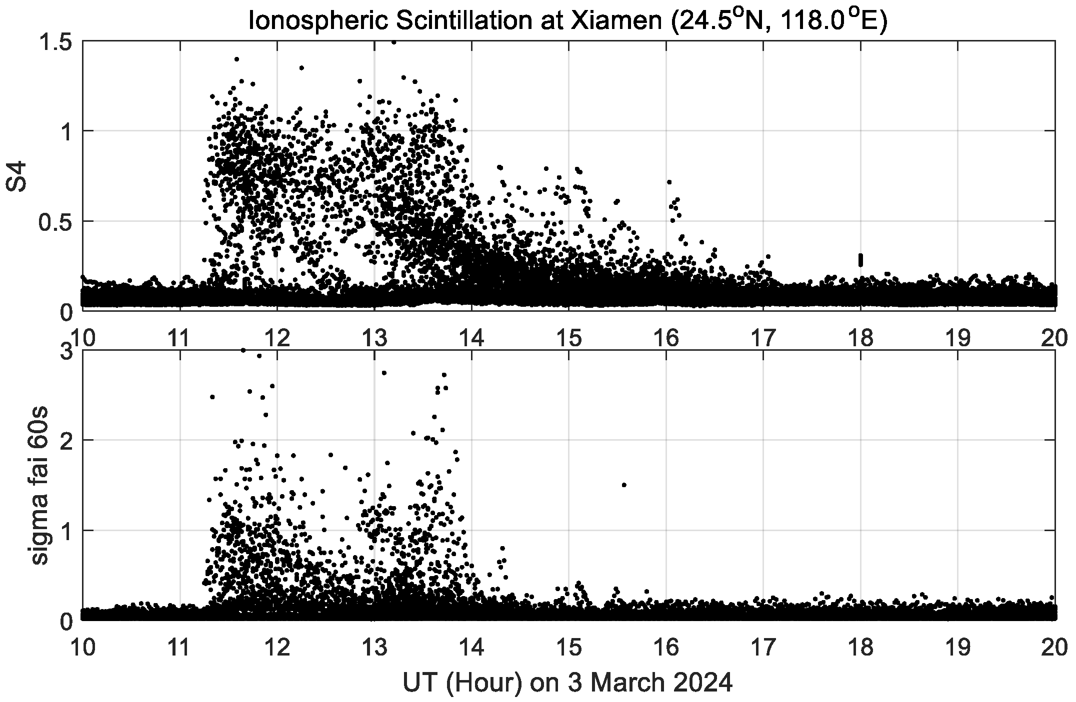
3.4. GNSS Scintillation

The GNSS scintillation receiver situated in Xiamen samples the amplitude and phase signals of all the navigation satellite systems at 50 Hz. The receiver recorded strong ionospheric scintillation on 3 March 2024. Figure 5 presents the amplitude and phase scintillation indices S₄ and ${\mathsf{\sigma }}_{\mathsf{\phi }}$. The amplitude scintillation began at about 11:15 UT, and continued until ~16:15 UT. The amplitude scintillation was extremely strong during 11:15–14:00 UT with S₄ > 1.0. After 14:00 UT, the strength of the scintillation became weaker but it remained relatively strong with S₄ > 0.7. During the period of scintillation, S₄ was weaker than 0.5 only at 15:30–16:00 UT. The phase scintillation was also strong between 11:15 and 14:00 UT. However, it disappeared at ~14:20 UT, two hours earlier than the amplitude scintillation.

The scintillation observations from BDS-GEO satellites provided the evolution of the ionospheric scintillation pattern at one fixed IPP. Figure 6 presents the S₄ index as observed by seven GEO satellites. The PRN number of the GEO satellites and the longitudes of the IPPs are shown in the title of each panel. From top to bottom, the IPPs were arranged in order from the west to the east. The latitudes of these IPPs were about 22.5° N.

It can be seen that the scintillation was first encountered by PRN 59 at 119.54° E, and then at 120.42° E and 122.51° E by PRN 1 and PRN 4, as shown by the red rectangle in Figure 6. The time delay of the scintillation pattern implied the EPBs drifted eastward. For this patch, the velocity estimated from the beginning time delay was about 430 m/s. But we should also note that the patch detected at 122.51° E was 40 min longer than that at 119.54° E, and S₄ during 11:25–11:45 UT was larger than those at 120.43° E.

For another patch, marked by the blue rectangle, PRN 60 and PRN 2 detected similar scintillation pattern. But at 117.35° E, ~350 km far from 114.11° E, the pattern was different, with two structures in one large patch. The eastward drift velocity was estimated to be ~100 m/s. The scintillation pattern at 109.68° E continued for ~200 min. But at the next east IPP of 114.11° E, it became very weak and the duration shrank to ~70 min.

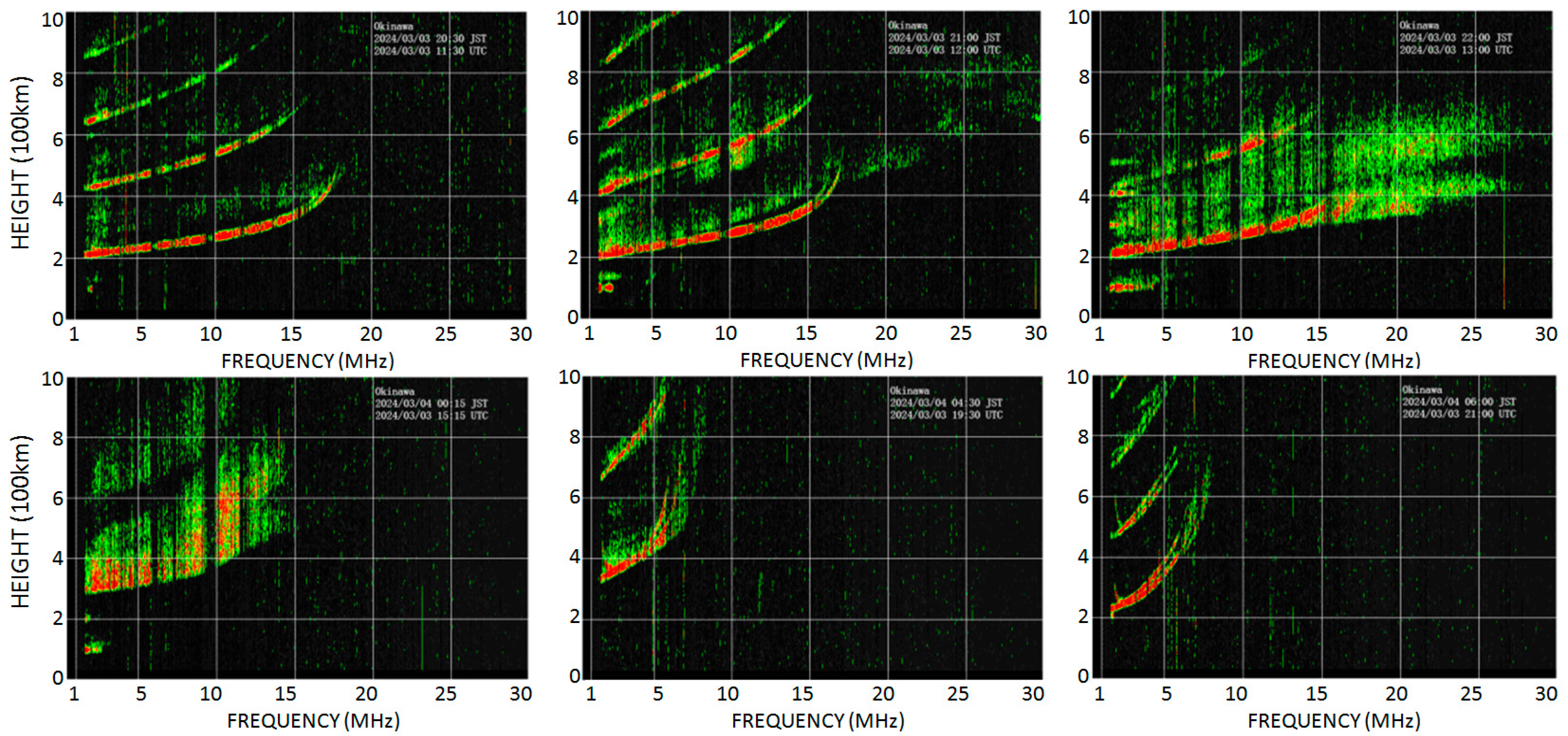
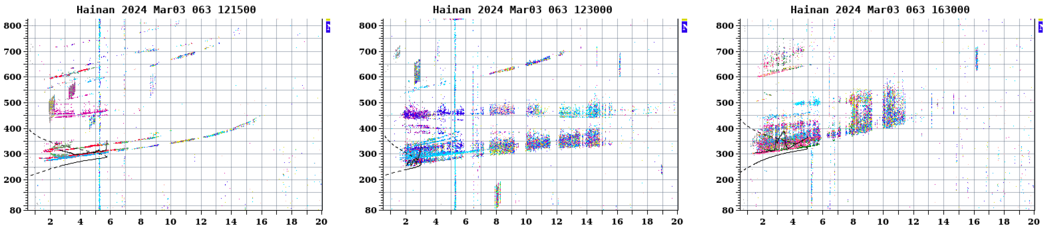
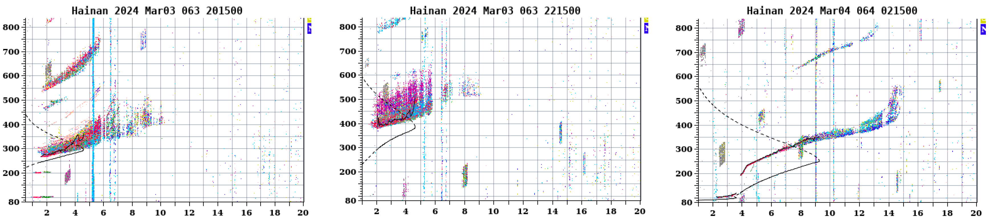
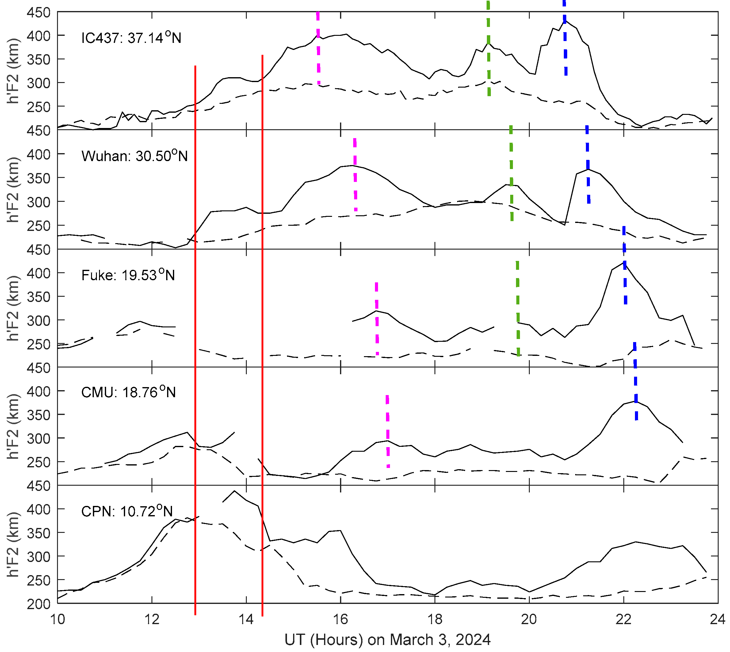
3.5. Spread F from Ionograms

Ionosondes at OKI, Fuke, CMU and CPN all detected SF on 3 March 2024. The ionosondes located in Wuhan (30.50° N, 114.48° E) did not detect SF. Therefore, it can be inferred that the equatorial spread F did not reach Wuhan. Here, we present the ionograms at OKI and Fuke as examples. The durations of SF observed at the two stations are listed in

Table 2. Spread F duration at OKI and Fuke.

Station ID	Geographic Latitude	Duration of Spread F (UT)	Data Gap (UT)
OKI	26.68° N	11:30–21:00	---
Fuke	19.53° N	12:15 3 March–02:15 4 March	14:15–16:15; 18:30–18:45 20:30–22:00; 02:30–03:30

.

Figure 7 shows the SF traces recorded at OKI. The SF began to appear at 11:30 UT. At 12:00 UT, the SF appeared at the frequencies beyond f_oF₂ (17 MHz), reaching 30 MHz. This type of SF was defined as strong range spread F (SSF), which is characterized by extended range spread on F layer echo traces extending beyond the local f_oF₂ value [13]. The spread trace beyond f_oF₂ developed more rapidly and became much stronger than that below f_oF₂ during 12:15–13:00 UT; then, the spread trace at the higher frequencies mixed with the range SF (RSF) at the lower frequencies. At 15:15 UT, the spread trace at higher frequency gradually vanished into normal RSF. After that, the RSF gradually evolved into frequency SF (FSF) and disappeared at 21:00 UT.

Figure 8 shows the appearance and evolution of the SF at Fuke (19.53° N, 109.13° E). Before the SF appeared, the ionosonde recorded the satellite trace at 12:15 UT, which continued until 13:00 UT. The SF appeared at 12:30 UT as SSF with the frequency extending to 15 MHz. At 16:30 UT, the extended frequency decreased, and the SF resembled normal RSF. Subsequently, the RSF evolved into FSF at 20:15 UT. During 20:30–22:00 UT, no observations were conducted. RSF was observed when the ionogram was recorded again at 22:15 UT. Then, the SF decayed and evolved into FSF, gradually disappearing after 02:15 UT on 4 March. The time 02:15 UT corresponds to ~09:30 LT at Fuke, meaning that the spread F persisted for at least 3 h after sunrise. The SF at Fuke lasted more than 5 h longer than that at OKI. It is regrettable that no ionogram was recorded during the data gap listed in Table 2. We are unable to determine how the SF developed during its evolution or what time the spread F disappeared. Nevertheless, we can suppose that the SF at 22:15 UT (05:30 LT) was associated with the freshly generated irregularities, because it appeared as RSF, which is different from the FSF at 20:15 UT. In this paper, we focus on the night-time ionospheric irregularities, and the SF event after 22:15 UT will be studied in the future.

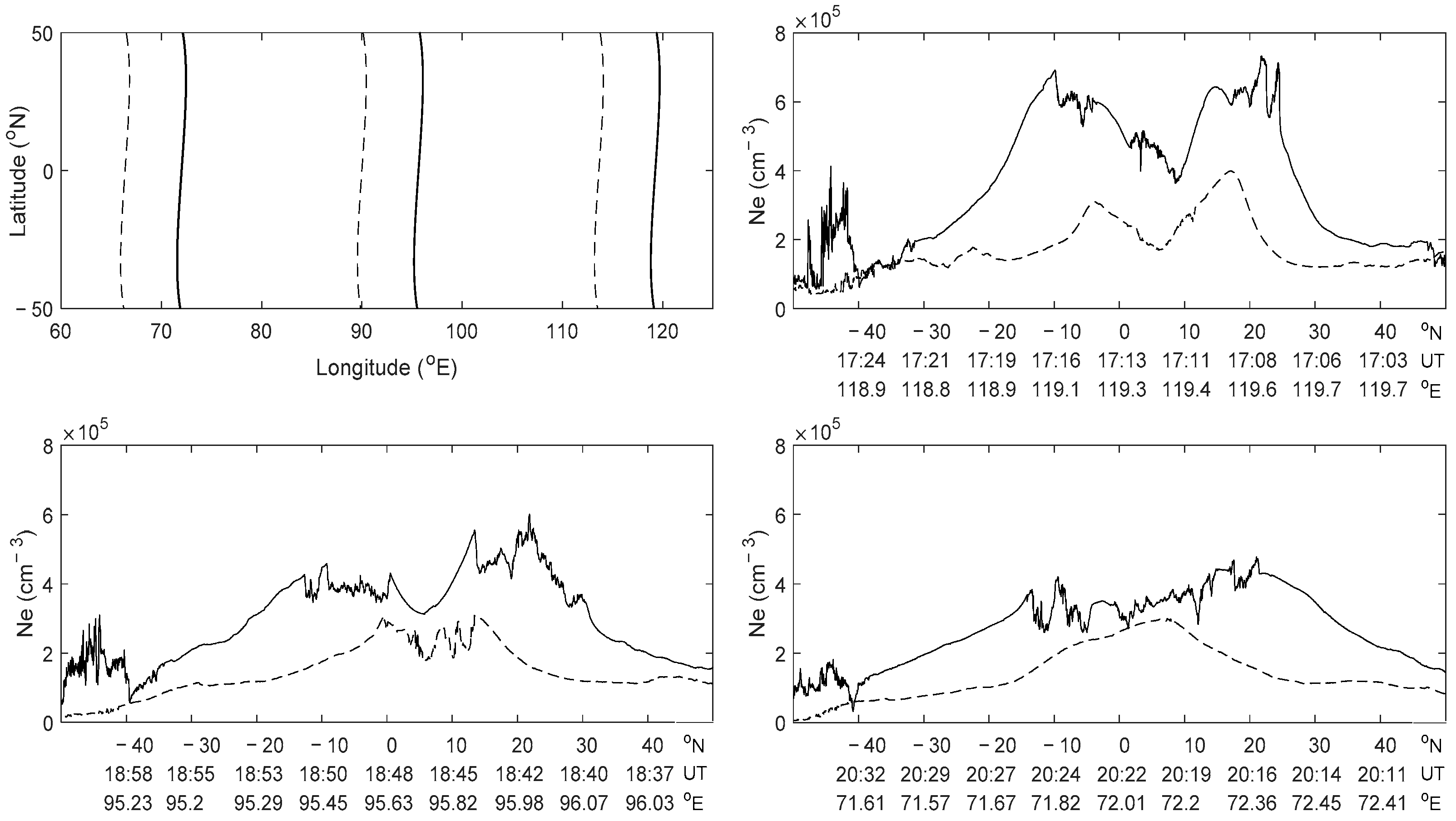
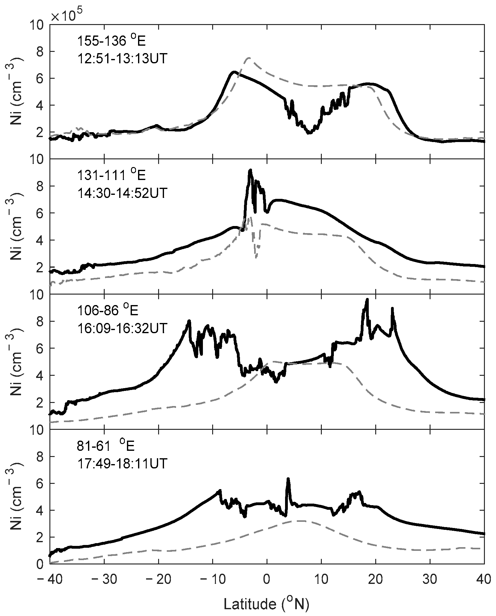
3.6. In Situ Measurements

Besides the ground-based observations, the in situ measurements by the SWARM-C and the FORMOSAT-5 satellites also detected EPBs. Figure 9 shows the number of electrons per cubic centimeter (Ne) detected by the SWARM-C satellite at an altitude of ~470 km. The satellite flew over the section at ~01:30 LT. Its orbit trace is shown in the left-top panel. The dashed/solid lines are the orbits on 2/3 March, respectively. The orbits on 3 March were about 30 min earlier than the references on 2 March. The other three panels present the Ne on 3 March (solid lines) and the references (dashed lines). The latitudes, UT and longitudes are labeled under the horizontal axis. It can be seen that on 3 March Ne enhanced and the crests of equatorial ionization anomaly (EIA) moved polarward. The EPBs were almost symmetric about the magnetic equator. Along the longitude of 95° E, the EPBs had the largest latitude extension, reaching 30° N.

The FORMOSAT-5 is at 720 km altitude along the 10:30/22:30 LT sector with a 2-day re-visit period. The ionospheric plasma concentrations (Ni) measured by the AIP on FORMOSAT-5 are shown in Figure 10. The solid line is the Ni on 3 March, and the dashed line shows the references on 1 March. The latitudes are labeled by the horizontal axis, and the corresponding UT and longitudes are marked on the top-left corner of each panel.

Between 12:51 and 13:12 UT, Ni was similar to the reference except for the electron density depletion accompanied by the bubbles near the magnetic equator. Two hours later, Ni at low to mid-latitudes became higher than the references. Along this orbit, no EPBs were detected. However, the TFTg and ROTI keograms detected EPBs in the same time period.

After 16:09 UT, Ni increased obviously, especially at the low latitudes. But near the magnetic equator, Ni had similar values to the references. The crests of EIA extended to higher latitudes compared with the references. At the same time, EPBs were detected near the south crest (−15–4° N) and north crest (10–23° N).

During the period 17:45–18:18 UT, the Ni values remained large but the difference with the references became smaller and the latitudinal range of the EPBs shrank.

4. Discussion

4.1. The Spatial Range and Scale of the EPBs

On the night of 3 March 2024, multi-instruments detected EPBs or equatorial irregularities. The longitudinal range was beyond our ground-based GNSS observation (93–123° E). In situ satellite measurements indicated that the longitudinal range of the EPBs was from ~70° E to ~150° E.

The measurements by the SWARM-C satellite, as shown in Figure 9, revealed that the EPBs along the longitude of ~96° E extended to 30° N at the altitude of ~470 km. The ground-based GNSS observations also showed that the EPBs extending to 30° N were located to the west of 105° E (the relevant figure is not presented in this paper due to the space limitation). However, the ionosonde at Wuhan (30.50° N, 114.48° E) did not detect SF. This could be attributed to the difference in longitudes. Wuhan is situated at 114.48° E, while the EPBs detected by the SWARM-C satellite and GNSS were located to the west of Wuhan. It is likely that the latitudinal extension of EPBs did not reach 30° N at the longitude of Wuhan.

As shown in Figure 10, FORMOSAT-5 did not detect EPBs at 14:40 UT near (20° N, 116° E), but the ground-based GNSS observed EPBs. This implied that the EPBs did not rise up to 720 km at 14:00 UT near 116° E. About 90 min later, FORMOSAT-5 detected EPBs near 95° E at the altitude of 720 km. The EPBs reached 23° N, with a corresponding apex height of ~1300 km. At 18:40 UT, the SWARM-C satellite detected EPBs extending to 30° N at the altitude of 480 km along 96° E. And the corresponding apex height was ~1700 km.

The ground-based GNSS observations showed that the irregularities included several patches, as illustrated in Figure 3 and Figure 4. However, there is an additional patch located at the top-left corner of Figure 4. The 1 s observations were re-sampled at 30 s intervals to calculate the ROTI in Figure 4. In Figure 3, the TFTg is derived from 1 s phase measurements. There were two possible explanations for these differences. Firstly, the 30 s and 1 s sampling rates represent irregularities with different scales. Assuming that the irregularities drifted at a speed of 100 m/s, 1 s sampling could detect irregularities with a scale of ~200 m, while the 30 s sampling interval was capable of detecting irregularities of the order of several kilometers [28]. In this paper, 30 s and 5 min time windows were employed to obtain the TFTg and ROTI, respectively, representing the irregularities with scales of several kilometers and tens of kilometers. Consequently, Figure 4 represents the irregularities with larger scales than those in Figure 3. The patch in the top-left corner of Figure 4 is composed of large-scale irregularities; these irregularities could not be measured by the TFTg using 1 s sampling. This patch was at the westernmost part of our observation range, and it may have drifted from the west of our observation range. During the later phase of EPBs, small-scale irregularities often decay and disappear earlier, whereas large-scale ones will persist for a longer time [29]. Secondly, the difference might be attributed to the distinct spatial ranges of TFTg and ROTI. The TFTg keogram was only based on the measurements from BDS-GEOs, resulting in IPPs located at the latitudes below ~24° N. In contrast, the ROTI keogram was based on both GEO and MEO satellites measurements, providing broader coverage. The top-left patch observed in Figure 4 likely corresponds to the ionospheric irregularities occurring at higher latitudes than those covered by the GEOs.

The scintillation receiver at Xiamen (24.5° N, 118.0° E) recorded different results using the amplitude scintillation index S₄ and phase scintillation index ${\mathsf{\sigma }}_{\mathsf{\phi }}$. The duration of the scintillation indentified by the S₄ index was longer than that identified by the ${\mathsf{\sigma }}_{\mathsf{\phi }}$ index. Previous research has pointed out that near the equatorial range, amplitude scintillation occurs more frequently than phase scintillation, and ${\mathsf{\sigma }}_{\mathsf{\phi }}$ is dominated by the deep fluctuation of electron density [30]. The earlier disappearance of the phase scintillation suggested that the deep fluctuation degraded earlier during the process of the evolution. The ROTI keogram shown in Figure 4 and the amplitude scintillation index S₄ in Figure 5 also demonstrate that the irregularity decayed as time elapsed.

Moreover, the amplitude scintillation disappeared at ~16:15 UT, and this result was consistent with the TFTg and ROTI keograms. However, the SF at Fuke persisted for a longer time compared to other observations. At the beginning of SF, the ionograms from Fuke and OKI detected a strong range-type spread F (SSF). At 16:30 UT, the SSF at Fuke decayed into normal RSF. Subsequently, it continued to decay gradually into mixed spread F (MSF) and frequency spread F (FSF). Sales et al. pointed out that SSF was related to the oblique echoes from the walls of EPB depletions [31]. The SSF had a good correlation with GNSS L-band scintillation in the low-latitude ionosphere, while FSF or MSF had no correlation with the occurrence of scintillation [13].

4.2. The Evolution of the EPBs

The whole lifetime of the EPBs in our GNSS observations was about 7 h. The EPBs appeared from east to west with sunset. During their lifetime, the EPBs drifted eastward, as shown in Figure 3 and Figure 4. The scintillation pattern also drifted eastward, as shown in Figure 6. But the drift velocity from the pattern marked by the red rectangle was much larger than those from the keograms and the pattern encircled by the blue rectangle. Based on the observed longer duration and stronger scintillation at 122.51° E, we can speculate that the freshly generated EPB merged with pre-existing eastward-drifting EPBs. Therefore, the estimated velocity was very large. But it was not the drift velocity of the scintillation pattern. The eastward drift velocity should be about 100–150 m/s.

The scintillation pattern marked by the blue rectangles split into two patterns at 117.35° E during its evolution process. Previous studies showed that the EPB can bifurcate during its development [32]. The splitting of two patterns may be associated with the bifurcation of EPB. When this pattern arrived at 122.51° E, the scintillation intensity significantly decreased, persisting for only ~15 min. During its evolution, the pattern underwent splitting followed by gradual decay.

The EPBs at all the GEO-IPPs trended to be intermittent. This may be associated with the eastward movement of the EPBs. The EPBs originated at different longitudes, and they drifted eastward during the evolution, so the irregularities detected at one GEO-IPP seemed to be intermittent.

The ionograms showed that the type of spread F was SSF first, and then it decayed into normal RSF, and finally vanished into FSF and disappeared. The result also implied that the irregularities became weaker and weaker during the evolution.

4.3. The Possible Physical Mechanism of the EPBs

Our observations showed that the EPBs first appeared at 11:15 UT at the longitude of ~120° E. Subsequently, the EPBs occurred successively from east to west, following the progression of sunset. The occurrence of the EPBs took place prior to the main phase of the geomagnetic storm. Therefore, the initial generation of the EPBs was not related to the geomagnetic storm. EPBs typically occur after sunset during equinox months in solar activity years.

To check the background of the ionosphere, the virtual heights of the F layer h’F from five ionosondes were manually scaled and are presented in Figure 11. From top to bottom, the latitudes decreased. The dashed lines are the mean heights on 1 and 2 March as references. The solid lines are h’F on 3 March 2024.

After sunset, the ionosphere at the lower latitudes (Fuke, CMU and CPN) was uplifted, as shown in Figure 11. The uplift at Fuke occurred earlier than that at CMU and CPU. This is because Fuke is located to the east of CMU and CPU, where the sunset is about one hour earlier. Such sunset ionospheric uplift was observed at low latitudes not only on the event day but also on the reference days. PRE of the eastward electric field is often thought to contribute to the uplift of the F layer and the generation of EPBs after sunset [9,33]. Therefore, it can be supposed that the generation of the EPBs was associated with the PRE.

At 12:50 UT, the main phase of the geomagnetic storm began. The ionosphere from low to mid-latitudes was uplifted simultaneously as shown by the two red solid lines. The uplift was more obvious at lower latitudes. The height enhancement continued for about 80 min. This may be associated with the storm-time PPEF.

Between 14:15 and 20:00 UT, the ionosphere experienced two additional uplifts. There was an obvious time delay from mid-latitudes to low latitudes, as shown by the magenta and green dashed lines in Figure 11. Unlike the ionospheric uplift caused by the eastward electric field, which is more pronounced at low latitudes, the two uplifts were more evident at mid-latitudes, showing a time delay from mid-latitudes to low latitudes. The two uplifts of the F layer might be associated with the storm-time equatorward neutral wind, which may play a role in the development of EPBs.

After 20:00 UT, ionosphere uplift was observed once more from mid- to low latitudes. This may contribute to the SF at Fuke after 22:00 UT, which was not the topic of this paper. We will focus on the morning spread F in another paper.

Before spread F, the ionogram at Fuke recorded the satellite traces, which were known ionogram signatures of a large-scale wave structure (LSWS) and a precursor for equatorial spread F [10]. Such satellite traces were also observed by the ionograms at the CMU and CPN stations, not only before but also during the spread F. This implied that the LSWS continued for several hours. It is speculated that the LSWS might play a role in seeding EPBs.

5. Conclusions

On 3 March 2024, ionospheric scintillation with S₄ > 1.0 was recorded for ~3 h by the scintillation receivers in Xiamen. The EPBs caused a lot of cycle slips and losses of lock in GNSS receivers within a longitudinal range of ~30 degrees, and this effect persisted for ~5 h. The ionograms showed strong range-type spread trace at frequencies beyond normal f_oF₂. During their development and evolution, the EPBs extended to 30° N at the altitude of ~470 km and drifted eastward at a speed of 100–150 m/s. A possible bifurcation phenomenon was observed during the evolution process of the EPBs.

The EPBs appeared before the main phase of the geomagnetic storm. Therefore, the initial generation of the EPBs should not be attributed to the geomagnetic storm, but rather to the PRE. With the beginning of the main phase, the height uplift was almost simultaneously observed from mid- to low latitudes, which might be related to the storm-time PPEF. During the main phase of the geomagnetic storm, two additional height uplifts with a time delay were observed from mid- to low latitudes and were assumed to be associated with the equatorward neutral wind. The mechanisms for the EPBs’ occurrence before and after the main phase of the storm were different. Before the main phase, PRE played a vital role in the occurrence of EPBs, while after the onset of the main phase, PPEF and neutral wind played significant roles in the development and survival of the EPBs, leading to strong scintillation, cycle slips and even loss of lock. The LSWS detected by the satellite traces on the ionograms may be the seeding source of the EPBs. More case studies and comparisons are required to better understand the impact of geomagnetic storms on EPBs.

References

1. Booker, H.G.; Wells, H.W. Scattering of radio waves by the F-region of the ionosphere. Terr. Magn. Atmos. Elec. 1938, 43, 249–256. [Google Scholar] [CrossRef]
2. Booker, H.G. Turbulence in the ionosphere with applications to meteortrails, radio-star scintillation, auroral radar echoes, and other phenomena. J. Geophys. Res. 1956, 61, 673–705. [Google Scholar] [CrossRef]
3. Woodman, R.F.; La Hoz, C. Radar observations of F region equatorial irregularities. J. Geophys. Res. 1976, 81, 5447–5466. [Google Scholar] [CrossRef]
4. Hanson, W.B.; Bamgboye, D.K. The measured motions inside equatorial plasma bubbles. J. Geophys. Res. 1984, 89, 8997. [Google Scholar] [CrossRef]
5. Hysell, D.L. An overview and synthesis of plasma irregularities in equatorial spread F. J. Atmos. Sol.-Terr. Phys. 2000, 62, 1037–1056. [Google Scholar] [CrossRef]
6. Meggs, R.W.; Mitchell, C.N.; Smith, A.M. An Investigation into the Relationship between Ionospheric Scintillation and Loss of Lock in GNSS Receivers. In Characterising the Ionosphere; Meeting Proceedings RTO-MP-IST-056, Paper 5; RTO: Neuilly-sur-Seine, France, 2006; pp. 5-1–5-10. Available online: http://www.rto.nato.int/abstracts.asp (accessed on 6 November 2009).
7. Zhang, D.; Cai, L.; Hao, Y.; Xiao, Z.; Shi, L.; Yang, G.; Suo, Y. Solar cycle variation of the GPS cycle slip occurrence in China low-latitude region. Space Weather 2010, 8, S10D10. [Google Scholar] [CrossRef]
8. Zhang, D.; Xiao, Z.; Feng, M.; Hao, Y.; Shi, L.; Yang, G.; Suo, Y. Temporal dependence of GPS cycle slip related to ionospheric irregularities over China low-latitude region. Space Weather 2010, 8, S04D08. [Google Scholar] [CrossRef]
9. Abdu, M.A. Day-to-day and short-term variabilities in the equatorial plasma bubble/spread F irregularity seeding and development. Prog. Earth Planet Sci. 2019, 6, 11. [Google Scholar] [CrossRef]
10. Tsunoda, R.T. Satellite traces: An ionogram signature for large-scale wave structure and a precursor for equatorial spread F. Geophys. Res. Lett. 2008, 35, L20110. [Google Scholar] [CrossRef]
11. Nishioka, M.; Saito, A.; Tsugawa, T. Occurrence characteristics of plasma bubble derived from global ground-based GPS receiver networks. J. Geophys. Res. 2008, 113, A05301. [Google Scholar] [CrossRef]
12. Li, G.; Ning, B.; Otsuka, Y.; Abdu, M.; Abadi, P.; Liu, Z.; Spogli, L.; Wan, W. Challenges to equatorial plasma bubble and ionospheric scintillation short- term forecasting and future aspects in East and Southeast Asia. Surv. Geophys. 2021, 42, 201–238. [Google Scholar] [CrossRef]
13. Shi, J.; Wang, G.; Reinisch, B.; Shang, S.; Wang, X.; Zherebotsov, G.; Potekhin, A. Relationship between strong range spread F and ionospheric scintillations observed in Hainan from 2003 to 2007. J. Geophys. Res. 2011, 116, A08306. [Google Scholar] [CrossRef]
14. Aarons, J. The role of the ring current in the generation or inhibition of equatorial F layer irregularities during magnetic storms. Radio Sci. 1991, 26, 1131–1149. [Google Scholar] [CrossRef]
15. Ma, G.; Maruyama, T. A super bubble detected by dense GPS network at East Asian longitudes. Geophys. Res. Lett. 2006, 33, L21103. [Google Scholar] [CrossRef]
16. Sun, W.; Li, G.; Lei, J.; Zhao, B.; Hu, L.; Zhao, X.; Li, Y.; Xie, H.; Li, Y.; Ning, B.; et al. Ionospheric super bubbles near sunset and sunrise during the 26–28 February 2023 geomagnetic storm. J. Geophys. Res. Space Phys. 2023, 128, e2023JA031864. [Google Scholar] [CrossRef]
17. Li, G.; Ning, B.; Hu, L.; Liu, L.; Yue, X.; Wan, W.; Zhao, B.; Igarashi, K.; Kubota, M.; Otsuka, Y.; et al. Longitudinal development of low-latitude ionospheric irregularities during the geomagnetic storms of July 2004. J. Geophys. Res. 2010, 115, A04304. [Google Scholar] [CrossRef]
18. Carter, B.A.; Yizengaw, E.; Pradipta, R.; Retterer, J.M.; Groves, K.; Valladares, C.; Caton, R.; Bridgwood, C.; Norman, R.; Zhang, K. Global equatorial plasma bubble occurrence during the 2015 St. Patrick’s Day storm. J. Geophys. Res. Space Phys. 2016, 121, 894–905. [Google Scholar] [CrossRef]
19. Nayak, C.; Tsai, L.C.; Su, S.Y.; Galkin, I.A.; Caton, R.G.; Groves, K.M. Suppression of ionospheric scintillation during St. Patrick’s Day geomagnetic super storm as observed over the anomaly crest region station Pingtung, Taiwan: A case study. Adv. Space Res. 2017, 60, 396–405. [Google Scholar] [CrossRef]
20. Kelley, M.C.; Fejer, B.; Gonzales, C. An explanation for anomalous equatorial ionospheric electric fields associated with a northward turning of the interplanetary magnetic field. Geophys. Res. Lett. 1979, 6, 301–304. [Google Scholar] [CrossRef]
21. Blanc, M.; Richmond, A. The ionospheric disturbance dynamo. J. Geophys. Res. 1980, 85, 1669–1686. [Google Scholar] [CrossRef]
22. Balan, N.; Liu, L.; Le, H. Brief review of equatorial ionization anomaly and ionospheric irregularities. Earth Planet Phys. 2018, 2, 1–19. [Google Scholar] [CrossRef]
23. Wu, K.; Qian, L.; Wang, W.; Cai, X.; Mclnerney, J.M. Investigation of the physical mechanisms of the formation and evolution of equatorial plasma bubbles during a moderate storm on 17 September 2021. Space Weather 2023, 21, e2023SW003673. [Google Scholar] [CrossRef]
24. Lin, Z.W.; Chao, C.K.; Liu, J.Y.; Huang, C.M.; Chu, Y.H.; Su, C.L.; Mao, Y.C.; Chang, Y.S. Advanced Ionospheric Probe scientific mission onboard FORMOSAT-5 satellite. Terr. Atmos. Ocean. Sci. 2017, 28, 99–110. [Google Scholar] [CrossRef]
25. Friis-Christensen, E.; Lühr, H.; Knudsen, D.; Haagmans, R. Swarm-an Earth observation mission investigating geospace. Adv. Space Res. 2008, 41, 210–216. [Google Scholar] [CrossRef]
26. Pi, X.; Mannucci, A.J.; Lindqwister, U.J.; Ho, C.M. Monitoring of global ionospheric irregularities using the worldwide GPS network. Geophys. Res. Lett. 1997, 24, 2283–2286. [Google Scholar] [CrossRef]
27. Ma, G.; Li, J.; Fan, J.; Wan, Q.; Maruyama, T.; Dong, L.; Gao, Y.; Zhang, L.; Wang, D. Observation of Post-Sunset Equatorial Plasma Bubbles with BDS Geostationary Satellites over South China. Remote Sens. 2024, 16, 3521. [Google Scholar] [CrossRef]
28. Aarons, J.; Mendillo, M.; Yantosca, R. GPS phase fluctuations in the equatorial region during the MISETA 1994 cmapaign. J. Geophys. Res. 1996, 101, 26851–26862. [Google Scholar] [CrossRef]
29. Basu, S.; Basu, S.; Aarons, J.; McClure, J.P.; Cousins, M.D. On the coexistence of kilometer- and meter-scale irregularities in the nighttime equatorial F-region. J. Geophys. Res. 1978, 83, 4219–4226. [Google Scholar] [CrossRef]
30. Beach, T.L. Perils of the GPS phase scintillation index (sf). Radio Sci. 2006, 41, RS5S31. [Google Scholar] [CrossRef]
31. Sales, G.S.; Reinisch, B.W.; Scali, J.L.; Dozois, C.; Bullett, T.W.; Weber, E.J.; Ning, P. Spread F and the structure of equatorial ionization depletions in the southern anomaly region. J. Geophys. Res. 1996, 101, 26819–26827. [Google Scholar] [CrossRef]
32. Yokoyama, T.; Shinagawa, H.; Jin, H. Nonlinear growth, bifurcation, and pinching of equatorial plasma bubble simulated by three-dimensional high-resolution bubble model. J. Geophys. Res. Space Phys. 2014, 119, 10474–10482. [Google Scholar] [CrossRef]
33. Patil, A.S.; Nade, D.P.; Taori, A.; Pawar, R.R.; Pawar, S.M.; Nikte, S.S.; Pawar, S.D. A Brief Review of Equatorial Plasma Bubbles. Space Sci. Rev. 2023, 219, 16. [Google Scholar] [CrossRef]
Figure 1. The geographic locations of the ground-based instruments. The dots represent the GNSS dual-frequency receivers, and * indicates the GNSS scintillation receivers.
Atmosphere 16 00218 g001
Figure 2. The variation in IMF-Bz and geomagnetic index SYM-H on 3–4 March 2024.
Atmosphere 16 00218 g002
Figure 3. TFTg keogram from BDS-GEO GION established by the NAOC on 3 March 2024. The colors represent different TFTg values, as shown by the colorbar. The magenta ellipses circled the five irregular patches.
Atmosphere 16 00218 g003
Figure 4. ROTI keogram from GPS, BDS and Galileo on 3 March 2024. Same as Figure 3 but for ROTI.
Atmosphere 16 00218 g004
Figure 5. Amplitude and phase scintillation indices at Xiamen on 3 March 2024.
Atmosphere 16 00218 g005
Figure 6. Amplitude scintillation detected by the GEOs of BDS at Xiamen on 3 March 2024. The red, blue and green rectangles mark three distinct groups of scintillation patterns caused by three patches.
Atmosphere 16 00218 g006
Figure 7. The spread F traces recorded by the ionograms at OKI on 3 March. The corresponding times are 11:30, 12:00, 13:00, 15:15, 19:30 and 21:00 UT, respectively.
Atmosphere 16 00218 g007
Figure 8. The ionograms recorded at Fuke, Hainan on 3–4 March 2024.
Atmosphere 16 00218 g008aAtmosphere 16 00218 g008b
Figure 9. EPBs detected by the SWARM-C satellites. The solid lines are the orbit traces and the Ne measurements during the EPB event, and the dash lines are the references.
Atmosphere 16 00218 g009
Figure 10. The ionospheric plasma concentrations (Ni) measured by the FORMOSAT-5. The solid lines show the Ni on 3 March, and the dashed lines represent the Ni on 1 March as references.
Atmosphere 16 00218 g010
Figure 11. The height variation of the ionosphere during the night-time on 3 March 2024. The solid black lines are h’F on 3 March 2024. In comparison, the dashed gray lines serve as references, indicating the mean heights on 1 and 2 March. The vertical lines in four different colors represent four uplifts of the F layer.
Atmosphere 16 00218 g011