Effects of Discretization of Smagorinsky–Lilly Subgrid Scale Model on Large-Eddy Simulation of Stable Boundary Layers

Abstract

Large-eddy simulation (LES) models are sensitive to numerical discretization because of the large fraction of resolved turbulent energy ($>80\%$) and the strong non-linear interactions between resolved-scale fields with the turbulence subgrid scale (SGS) model. The effects of the Smagorinsky–Lilly SGS model discretization are investigated. Three finite difference schemes are compared. Second-, fourth-, and sixth-order centered difference schemes are used to approximate the spatial derivatives of the SGS model. In the LES of homogeneous isotropic turbulence (HIT), including (non-isotropic) turbulent mixing of a passive scalar, no differences are observed with respect to the SGS model discretization. The HIT LES results are validated against a direct numerical simulation, which resolves all flow scales and does not include an SGS model. In the LES of a moderately stable atmospheric boundary layer, the LES results depend on the SGS discretization for coarse grid resolutions. The second-order scheme performs better at coarse resolutions compared to higher-order schemes. Overall, it is found that higher-order discretizations of the Smagorinsky–Lilly model are not beneficial compared to the second-order scheme.

1. Introduction

Large-eddy simulation (LES) is a turbulent-flow modeling technique that resolves most of the energetic flow motions [1,2,3,4]. The effects of the smaller motions are parameterized through a subgrid scale (SGS) model. “SGS model” in the general LES literature is synonymous to “turbulence parametrization”, which is a term typically used in the geophysical sciences. In the formulation of SGS models, the smaller scales are assumed to be generic in nature without any complex coherent structure. One of the first SGS models, still used in geophysical LES, is based on the form originally introduced by Smagorinsky [5] and later formally derived for three-dimensional turbulence by Lilly [6,7].

Many SGS models are based on two key components: the model formulation and a specific relation that provides closure. The model formulation contains the underlying assumptions of the SGS turbulence. The Smagorinsky–Lilly model is based on an SGS stress tensor that is similar to Newtonian viscous stress with an “eddy diffusivity” coefficient in place of the fluid kinematic viscosity. The value of the eddy diffusivity is determined by considering a homogeneous and isotropic SGS flow with a Kolmogorov-type spectrum $E\left(k\right)$, where k is the wavenumber-vector magnitude. Closure is attained by integrating the spectrum to determine the local dissipation (see [6,7] for details). In LES SGS models, the grid spacing is part of the model formulation because it is needed to estimate the resolved scale and SGS parts of flow-related quantities, such as the turbulent kinetic energy. Depending on the SGS model formulation, the cut-off length scale separating the resolved and SGS flow is not always the grid spacing but is typically related to it. This is how the model becomes “scale-aware” and the amount of unresolved turbulent energy is estimated. For example, in the process of determining the model constant, Lilly [6] (Equation (3.6)) relates the square of the rate-of-strain tensor D as an integral over the resolved-scale wavenumbers of the dissipation spectrum

$$D^2\approx 4{\int }_0^{\pi /l}{k}^{2}E\left(k\right)\mathrm{d}k,$$

(1)

Ref. [6] states that “$\pi /l$ is the largest wavenumber unambiguously representable on the grid”. The length scale l is expected to be comparable to the grid spacing $l\approx \Delta x$. The range of wavenumbers accurately represented on the grid is referred to as the resolving power of the numerical approximation [8,9,10]. The practical implications of such a simple statement are complex, because partitioning the field into resolved and SGSs generates several extra terms in the evolution equations of the resolved-scale field, as shown by Leonard [11]. Most of the LES implementations lump all extra terms into the turbulence model, even though some of these effects are related to discretization choices (e.g., type of filter used, numerical grid geometry, boundary conditions, and truncation error of the discrete derivative operators). For simple flows, several past studies explored these interactions between numerical error and SGS model performance, e.g., [12,13,14,15,16].

In the LES of moderately stable atmospheric boundary layers, Matheou [10] found that, in practice, relatively small SGS model constant adjustments are required compared to changes in the resolving power of the numerical spatial derivative approximation. For instance, the resolving efficiency increases by more than a factor of 4 between the second- and sixth-order advection schemes, but the corresponding adjustment in the model characteristic length scale is only about 1.5. Matheou [10] only considers different advection term discretizations and uses second-order centered differences to discretize the SGS terms. The present study expands the numerical model error investigation of [10] to the SGS model discretization effects.

Because of the diffusive nature of the SGS terms, large discrepancies are not expected between various orders of finite-difference approximations. However, given the observed sensitivity of the Smagorinsky–Lilly SGS model in the LES of stable boundary layers with respect to discretization [10], some result variability is possible. Two types of turbulent flows are considered: (a) homogeneous isotropic turbulence (HIT) and (b) a stable atmospheric boundary layer. Both types of flows include turbulent mixing of a scalar. In HIT, the scalar is passive, and in the stable boundary layer, the scalar is active. The direct numerical simulation (DNS) and LES of HIT are carried out; however, the DNS results are used for LES validation. Stable boundary layer LES results are compared with respect to their relative differences. Section 2 describes the flow configuration and DNS and LES numerical models, including the SGS discretization. The results are presented in Section 3 and conclusions are summarized in Section 4.

2. Methodology

2.1. Homogeneous Isotropic Turbulence Direct Numerical Simulation

A DNS of decaying homogeneous isotropic turbulence is used as a reference for the LES model. The DNS includes mixing of a passive scalar. Passive scalar fluctuations are produced by a mean scalar gradient $\beta =\mathrm{d}\langle \Phi \rangle /\mathrm{d}z$ in the vertical z direction as in [17]. The angle brackets denote the average in a horizontal, x–y, plane. The conservation equations of mass, momentum, and passive scalar fluctuation $\varphi$ in an incompressible fluid with uniform density $\rho =1$ are

$${\displaystyle \frac{\partial u_i}{\partial x_i}}=0,$$

(2)

$${\displaystyle \frac{\partial u_i}{\partial t}}+{\displaystyle \frac{\partial u_i{u}_j}{\partial x_j}}=-{\displaystyle \frac{\partial p}{\partial x_i}}+\nu {\displaystyle \frac{{\partial }^2{u}_i}{\partial x_j^2}},$$

(3)

$${\displaystyle \frac{\partial \varphi }{\partial t}}+\beta u_3+{\displaystyle \frac{\partial \varphi u_j}{\partial x_j}}=\Gamma {\displaystyle \frac{{\partial }^2\varphi }{\partial x_j^2}},$$

(4)

where $\beta =1$, $[u_1,u_2,u_3]$ is the velocity vector in Cartesian coordinates $[x_1,x_2,x_3]$ or $[x,y,z]$, p is the pressure, $\nu$ is the kinematic viscosity, $\Gamma$ is the scalar diffusivity coefficient, and the Prandlt number is $Pr=\nu /\Gamma =0.7$.

The flow is simulated in a cubical triply periodic domain with sides $2\pi$ and grid size ${1024}^3$. The velocity field is initialized with a snapshot of a forced homogeneous isotropic turbulence DNS on a ${1024}^3$ grid from the Johns Hopkins Turbulence Database [18,19]. The simulation is run for an initial “spin up” time period of 2 turn-over times based on the forced steady-state HIT. During this time, the scalar field develops turbulent fluctuations and the velocity field adjusts to the (somewhat) different fluid-flow solver. The spectral code of [20] is used for the DNS.

There is no production mechanism of turbulent kinetic energy, $\mathrm{TKE}={\displaystyle \frac{1}{2}}(\overline{uu}+\overline{vv}+\overline{ww})$; thus, TKE decays with respect to time. The overbars denote instantaneous volume-averaged variables in the DNS. The initial (after the “spin up”) Taylor Reynolds number is $R{e}_{\lambda }=230$ and decreases to $R{e}_{\lambda }=80$ at the end of the run. The DNS is well resolved throughout the simulations with the product of the maximum (dealiased) wavenumber and the Kolmogorov scale $k_{\max }\eta =1.2$ initially. As the flow evolves, the turbulence decays and the Kolmogorov scale increases. At the end of the simulation, $k_{\max }\eta =4$. The scalar includes a production term $\beta u_3$, and scalar variance ${\displaystyle \frac{1}{2}}\overline{\varphi \varphi }$ does not decay as the Reynolds number decreases. All HIT flow statistics used in this study only depend on time. The HIT LES runs (see following section) are initialized from the snapshot of the DNS. After the initial “spin up” period, the DNS flow fields are coarsened and used as the initial condition for the LES with various grid resolutions (see Section 2.2). The DNS fields are coarsened by applying a sharp spectral cut-off filter. Four LES grid resolutions are used: ${32}^3$, ${64}^3$, ${128}^3$, and ${256}^3$. Figure 1 shows x–z planes from the coarsened scalar fields used to initialize the LES. The LES grid resolution varies by a factor of 8 and includes fields without any small-scale structure (grid ${32}^3$) to fields with fine structures (grid ${256}^3$).

TKE and scalar variance are used to compare the DNS and LES. The SGS stress tensor of the Smagorinsky–Lilly model has zero trace; thus, the SGS TKE is not available in the LES. The comparison between the LES and DNS is performed only using the LES resolved-scale fields. This is accomplished by computing the TKE and scalar variance in the DNS at scales larger than the LES grid resolution by integrating the three-dimensional spectrum, e.g., $\mathrm{TKE}(t)={\int }_0^{\pi /\Delta x}E(t,k)\mathrm{d}k$.

2.2. Large-Eddy Simulation

Two LES model configurations are used. The first corresponds to HIT, including passive scalar mixing, which is the LES counterpart of the DNS described in Section 2.1. The second corresponds to the GABLS 1 stable atmospheric boundary layer case [21]. The filtered (density-weighted) anelastic approximation of the Navier–Stokes equations [22,23] is used in the LES. The conservation equations for mass, momentum, and potential temperature written on the f-plane are, respectively,

$${\displaystyle \frac{\partial {\overline{\rho }}_0{\tilde{u}}_i}{\partial x_i}}=0,$$

(5)

$${\displaystyle \frac{\partial {\overline{\rho }}_0{\tilde{u}}_i}{\partial t}}+{\displaystyle \frac{\partial \left({\overline{\rho }}_0{\tilde{u}}_i{\tilde{u}}_j\right)}{\partial x_j}}=-{\theta }_0\overline{{\rho }_0}{\displaystyle \frac{\partial {\overline{\pi }}_2}{\partial x_i}}+{\delta }_{i3}g{\displaystyle \frac{{\overline{\rho }}_0(\tilde{\theta }-\langle \tilde{\theta }\rangle )}{{\theta }_0}}-{ϵ}_{ijk}{\overline{\rho }}_0{f}_j({\tilde{u}}_k-u_{g,k})-{\displaystyle \frac{\partial {\tau }_{ij}}{\partial x_j}}+{\displaystyle \frac{\partial {\tilde{d}}_{ij}}{\partial x_j}},$$

(6)

$${\displaystyle \frac{\partial {\overline{\rho }}_0\tilde{\theta }}{\partial t}}+{\displaystyle \frac{\partial {\overline{\rho }}_0\tilde{\theta }{\tilde{u}}_j}{\partial x_j}}=-{\displaystyle \frac{\partial {\sigma }_j}{\partial x_j}}+{\displaystyle \frac{\partial }{\partial x_j}}\left({\rho }_0\Gamma {\displaystyle \frac{\partial \tilde{\theta }}{\partial x_j}}\right),$$

(7)

where $d_{ij}$ is the viscous stress tensor, ${\pi }_2$ is the dynamic Exner function that satisfies the anelastic constraint (2) (see [10]), and ${\theta }_0$ is the (constant) basic-state potential temperature. The SGS stress tensor ${\tau }_{ij}$ and temperature flux ${\sigma }_j$ are estimated using the Smagorinsky–Lilly turbulence model (see Section 2.3). Buoyancy is proportional to deviations in potential temperature from its instantaneous horizontal average, $\langle \theta \rangle$. In the LES, overbars denote spatially filtered variables [11] and tildes denote Favre-filtered variables, e.g., $\tilde{\theta }\equiv \overline{\rho \theta }/\overline{\rho }$. A fourth-order centered (non-dissipative) fully conservative scheme [10,24] is used to discretize the momentum and scalar advection term. The third-order Runge–Kutta method of [25] is used to advance the governing equations in time, both in the DNS and LES.

In the LES of HIT, the density is constant and drops out of the equations. The buoyancy term is not included in the momentum equations; thus, $\theta$ becomes a passive scalar. Also, the Coriolis term is not present in the momentum equation. The viscous terms are identical to those in (3) and (4). The mean scalar gradient term $\beta u_3$ is added to the LHS of (7). In the LES of HIT, the velocity field and scalar are initialized from the coarsened DNS fields (see Section 2.1). The boundary conditions are triply periodic as in the DNS. In the stable boundary layer, the LES runs follow the case of [21]. The boundary layer is driven by geostrophic wind in the zonal direction $u_g=8\mathrm{m}{\mathrm{s}}^{-1}$. The latitude is 73° N. A surface cooling of $0.25\mathrm{K}{\mathrm{h}}^{-1}$ is prescribed. The lapse rate above the boundary layer is $0.01\mathrm{K}{\mathrm{m}}^{-1}$. Surface fluxes are computed using Monin–Obukhov similarity theory, which relates the resolved-scale vertical gradient at the surface with the surface turbulent fluxes. For stable conditions, the wind profile is

$${\tilde{U}}_h\left(z\right)={\displaystyle \frac{u_{*}}{\kappa }}\left(ln{\displaystyle \frac{z}{z_0}}+4.8{\displaystyle \frac{z}{L}}\right),$$

(8)

and the potential temperature is

$$\tilde{\theta }\left(z\right)=\tilde{\theta }\left(0\right)+{\displaystyle \frac{{\theta }_{*}}{\kappa }}\left(ln{\displaystyle \frac{z}{z_0}}+7.8{\displaystyle \frac{z}{L}}\right),$$

(9)

where ${\tilde{U}}_h$ is the wind speed, $\kappa =0.4$ is the von Karman constant, $z_0=0.1\mathrm{m}$ is the surface roughness length, L is the Obukhov length, $u_{*}$ is the friction velocity, and ${\theta }_{*}$ is the temperature scale. At each $(x,y)$ location, by using the values of ${\tilde{U}}_h(z=\Delta z/2)$ and $\tilde{\theta }(z=\Delta z/2)$ in (8) and (9), $u_{*}$ and ${\theta }_{*}$ can be computed and, subsequently, the momentum and heat surface fluxes.

Doubly periodic boundary conditions are used in the horizontal directions and a sponge layer is present at the top of the computational domain to inhibit unwanted gravity wave reflections (see [10] for details). The domain size is $1.{024}^2\times 0.4{\mathrm{km}}^3$. Three grid resolutions are used: $\Delta x=2$, 4, and $8\mathrm{m}$. The grid resolution is uniform and isotropic: $\Delta x=\Delta y=\Delta z$.

2.3. Subgrid-Scale Model Discretization

The Smagorinsky–Lilly model uses an eddy diffusivity assumption to parameterize the SGS stress tensor:

$${\tau }_{ij}=-2{\overline{\rho }}_0{\nu }_t{\tilde{D}}_{ij},$$

(10)

and turbulent scalar flux:

$${\sigma }_j=-{\rho }_0{\displaystyle \frac{{\nu }_t}{P{r}_t}}{\displaystyle \frac{\partial \tilde{\theta }}{\partial x_j}},$$

(11)

where $P{r}_t=0.33$ is the model’s turbulent Prandtl number. The eddy diffusivity is parameterized as

$${\nu }_t={\Delta }^2{\left({\tilde{D}}_{ij}{\tilde{D}}_{ij}\right)}^{1/2}{f}_m.$$

(12)

The zero-trace resolved-scale rate of strain tensor $\tilde{D}$ is

$${\tilde{D}}_{ij}={\displaystyle \frac{1}{2}}\left({\displaystyle \frac{\partial {\tilde{u}}_i}{\partial x_j}}+{\displaystyle \frac{\partial {\tilde{u}}_j}{\partial x_i}}\right)-{\displaystyle \frac{1}{3}}{\delta }_{ij}{\displaystyle \frac{\partial {\tilde{u}}_k}{\partial x_k}}.$$

(13)

The characteristic SGS length-scale $\Delta$ is the product of the model constant $C_s$ and the grid spacing $\Delta x$:

$$\Delta =C_s\Delta x.$$

(14)

Near the surface, the characteristic length scale is modified to account for the confinement of the SGS eddies [26]:

$${\displaystyle \frac{1}{{\Delta }^2}}={\displaystyle \frac{1}{{(C_s\Delta x)}^2}}+{\displaystyle \frac{1}{{\left({\kappa }_{v}z\right)}^2}},$$

(15)

where ${\kappa }_v=0.4$ is the von Kármán constant and z is the height from the surface. For stably and unstably stratified flows, the function $f_m$ adjusts the turbulent viscosity based on the local flow stratification [27]:

$$\begin{array}{cc}{f}_m={(1-Ri/P{r}_t)}^{1/2}\hfill & Ri/P{r}_t<1\hfill \\ f_m=0\hfill & Ri/P{r}_t\ge 1,\hfill \end{array}$$

(16)

where $Ri=N^2/{\left|\tilde{D}\right|}^2$ is the gradient Richardson number and N is the buoyancy frequency.

The value of the model constant $C_s$ is found to depend on the flow usually requiring some model “tuning” depending on the application, e.g., [28]. In the HIT LES, we use $C_s=0.18$ because it is close to the theoretical value [6,7,10]. The Smagorinsky–Lilly model is essentially exact for HIT and, in numerical sensitivity experiments (not shown here), the results are almost identical in HIT LES using $C_s=0.18$–$0.23$. In the LES of the stable atmospheric boundary layer, $C_s=0.2$ is used based on the results of the parametric study of [10].

The governing equations are discretized on an Arakawa C (staggered) grid [29,30]. The SGS stress tensor $\tau$ and fluxes $\sigma$ are discretized using the “SMC” variable configuration of [31]. Figure 2 shows the variable arrangement on the computational grid. All thermodynamic (scalar) variables, including pressure, are defined at the cell center. The velocity components are located at the center of cell faces. The elements of the SGS scalar flux vector $\sigma$ are computed at the same location as the velocity vector. The off-diagonal elements of the SGS stress tensor $\tau$ are located on the cell edges and the diagonal elements of $\tau$ are located at the center of the cell faces. The variable arrangement results in a natural staggering of variables where derivatives are computed without the need for interpolation.

The approximation of the SGS terms in the governing equations includes three components: (a) the approximation of $\tilde{D}$ and the scalar flux $\partial \tilde{\theta }/\partial x_j$, (b) estimating ${\nu }_t$ at different locations, and (c) approximating the divergence of $\tau$ and $\sigma$. Approximations for the velocity derivatives in $\tilde{D}$ and the divergence are straightforward because, by using the model variable arrangement of Figure 2, the location of the derivative is either at the same discrete function positions or at the midpoint between grid function values. Note that the model uses a grid with constant $\Delta x$, $\Delta y$, and $\Delta z$. The present discussion only applies to grids with constant grid spacing. The centered difference scheme which approximates the derivative at the locations of the grid function is

$${\delta }_i\varphi ={\displaystyle \frac{1}{\Delta x}}[{\alpha }_1({\varphi }_{i+1}-{\varphi }_{i-1})+{\alpha }_2({\varphi }_{i+2}-{\varphi }_{i-2})+{\alpha }_3({\varphi }_{i+3}-{\varphi }_{i-3})],$$

(17)

and that at the midpoints is

$${\delta }_{{\displaystyle \frac{1}{2}}}\varphi ={\displaystyle \frac{1}{\Delta x}}[{\beta }_1({\varphi }_{i+{\displaystyle \frac{1}{2}}}-{\varphi }_{i-{\displaystyle \frac{1}{2}}})+{\beta }_2({\varphi }_{i+{\displaystyle \frac{3}{2}}}-{\varphi }_{i-{\displaystyle \frac{3}{2}}})+{\beta }_3({\varphi }_{i+{\displaystyle \frac{5}{2}}}-{\varphi }_{i-{\displaystyle \frac{5}{2}}})].$$

(18)

Table 1. Coefficients of the finite difference schemes used in the approximation of the subgrid scale terms.

Order	${\mathit{\alpha }}_1$	${\mathit{\alpha }}_2$	${\mathit{\alpha }}_3$	${\mathit{\beta }}_1$	${\mathit{\beta }}_2$	${\mathit{\beta }}_3$
Second	${\displaystyle \frac{1}{2}}$	0	0	1	0	0
Fourth	${\displaystyle \frac{8}{12}}$	$-{\displaystyle \frac{1}{12}}$	0	${\displaystyle \frac{27}{24}}$	$-{\displaystyle \frac{1}{24}}$	0
Sixth	${\displaystyle \frac{45}{60}}$	$-{\displaystyle \frac{9}{60}}$	${\displaystyle \frac{1}{60}}$	${\displaystyle \frac{2250}{1920}}$	$-{\displaystyle \frac{125}{1920}}$	${\displaystyle \frac{9}{1920}}$

shows the coefficient values to construct schemes of different orders. Relation (17) corresponds to the standard centered finite differences up to the sixth order.

To better illustrate the approximation of the stress tensor divergence, ${\displaystyle \frac{\partial {\tau }_{ij}}{\partial x_j}}$, in the momentum equation, we use the following example for a two-dimensional case. To time-advance $u_{i+{\displaystyle \frac{1}{2}},j}$ the y-derivative of ${\tau }_{12}$ at the $(i+{\displaystyle \frac{1}{2}},j)$ location, denoted by ${\displaystyle \frac{\partial {\tau }_{12}}{\partial y}}{|}_{i+{\displaystyle \frac{1}{2}},j}$, is needed. For the second-order scheme (from Table 1: ${\beta }_1=1$, ${\beta }_2=0$, and ${\beta }_3=0$), this is approximated as

$${\displaystyle \frac{\partial {\tau }_{12}}{\partial y}}{|}_{i+{\displaystyle \frac{1}{2}},j}\approx {\delta }_{y,{\displaystyle \frac{1}{2}}}{\tau }_{12}={\displaystyle \frac{1}{\Delta y}}{\beta }_1\left({\tau }_{12,i+{\displaystyle \frac{1}{2}},j+{\displaystyle \frac{1}{2}}}-{\tau }_{12,i+{\displaystyle \frac{1}{2}},j-{\displaystyle \frac{1}{2}}}\right)+O(\Delta y^2).$$

(19)

The elements of the stress tensor are estimated using (10)

$${\tau }_{12,i+{\displaystyle \frac{1}{2}},j+{\displaystyle \frac{1}{2}}}=-2{\rho }_{j+{\displaystyle \frac{1}{2}}}{\nu }_t{\tilde{D}}_{12i+{\displaystyle \frac{1}{2}},j+{\displaystyle \frac{1}{2}}}=-{\rho }_{j+{\displaystyle \frac{1}{2}}}{\nu }_t\left({\displaystyle \frac{\partial u}{\partial y}}{|}_{i+{\displaystyle \frac{1}{2}},j+{\displaystyle \frac{1}{2}}}+{\displaystyle \frac{\partial v}{\partial x}}{|}_{i+{\displaystyle \frac{1}{2}},j+{\displaystyle \frac{1}{2}}}\right).$$

(20)

The density at the full model levels $(j+{\displaystyle \frac{1}{2}})$ is estimated using the same interpolation polynomial as the momentum scheme. The turbulent viscosity coefficient is also interpolated at the location of ${\tau }_{12}$, but to simplify the discussion and notation, it appears without any subscripts

$${\tau }_{12,i+{\displaystyle \frac{1}{2}},j+{\displaystyle \frac{1}{2}}}\approx -\rho {\nu }_t\left({{\delta }_{y}u|}_{i+{\displaystyle \frac{1}{2}},j+{\displaystyle \frac{1}{2}}}+{{\delta }_{x}v|}_{i+{\displaystyle \frac{1}{2}},j+{\displaystyle \frac{1}{2}}}\right)+O(\Delta x^2,\Delta y^2).$$

(21)

The velocity derivatives are discretized using the same order as the divergence of $\tau$. For the second-order scheme approximation of (17),

$${\tau }_{12,i+{\displaystyle \frac{1}{2}},j+{\displaystyle \frac{1}{2}}}\approx -\rho {\nu }_t\left({\displaystyle \frac{1}{\Delta y}}{\alpha }_1(u_{i+{\displaystyle \frac{1}{2}},j+1}-u_{i+{\displaystyle \frac{1}{2}},j})+{\displaystyle \frac{1}{\Delta x}}{\alpha }_1(v_{i+1,j+{\displaystyle \frac{1}{2}}}-v_{i,j+{\displaystyle \frac{1}{2}}})\right).$$

(22)

The locations of the velocity components in (22) are the natural locations of the velocity grid function and no interpolation is required. The drawback of the present discretization is that multiple evaluations of the same velocity derivatives are required at different locations on the grid. This small increase in computational cost is compensated by the good numerical properties of the discretization [31].

Because of the dual application of the first derivative finite difference (17) and (18), higher-order schemes result in comparatively large stencils spanning all directions. In contrast, the second-order scheme is relatively compact in space, using local information to estimate the SGS turbulent-flow properties.

In the atmospheric boundary layer LES, a slip and no-penetration surface boundary condition is imposed for the resolved-scaled fields. To avoid changing the finite difference schemes near the wall, ghost or halo cells are used to impose the boundary conditions. The boundary condition corresponds to the surface being an anti-symmetry plane for the vertical velocity $\tilde{w}\left(z\right)=-\tilde{w}(-z)$ and a symmetry plane for all other variables, e.g., $\tilde{u}\left(z\right)=\tilde{u}(-z)$, or ${\displaystyle \frac{\partial \tilde{u}}{\partial z}}$ at $z=0$.

Estimating ${\nu }_t$ at the cell centers uses (18) to approximate the velocity derivatives of ${\tilde{D}}_{ij}$ with an additional interpolation step for the cross-derivative terms, e.g., $\partial u/\partial y$. The interpolation matches the order of the derivative approximation. The eddy viscosity is interpolated on cell faces and edges using averages or the nearest two (on cell faces) or four values (on cell edges).

Table 2. Simulation summary. The horizontal grid points are $N_x$ and vertical grid points at $N_z$. The grid spacing $\Delta x$ is uniform in all directions, $C_s$ is the Smagorinsky constant, and “Order” denotes the order of accuracy of the SGS term discretization.

Name	Type	Flow	${\mathit{N}}_{\mathit{x}}$	${\mathit{N}}_{\mathit{z}}$	$\mathbf{\Delta }\mathit{x}$	${\mathit{C}}_{\mathit{s}}$	Order
D	DNS	HIT	1024	1024	$2\pi /1024$	–	–
H2-32	LES	HIT	32	32	$2\pi /32$	0.18	Second
H2-64	LES	HIT	64	32	$2\pi /64$	0.18	Second
H2-128	LES	HIT	128	32	$2\pi /128$	0.18	Second
H2-256	LES	HIT	256	32	$2\pi /256$	0.18	Second
H4-32	LES	HIT	32	32	$2\pi /32$	0.18	Fourth
H4-64	LES	HIT	64	64	$2\pi /64$	0.18	Fourth
H4-128	LES	HIT	128	128	$2\pi /128$	0.18	Fourth
H4-256	LES	HIT	256	256	$2\pi /256$	0.18	Fourth
H6-32	LES	HIT	32	32	$2\pi /32$	0.18	Sixth
H6-64	LES	HIT	64	64	$2\pi /64$	0.18	Sixth
H6-128	LES	HIT	128	128	$2\pi /128$	0.18	Sixth
H6-256	LES	HIT	256	256	$2\pi /256$	0.18	Sixth
S2-128	LES	ABL	128	50	8	0.2	Second
S2-256	LES	ABL	256	100	4	0.2	Second
S2-512	LES	ABL	512	200	2	0.2	Second
S4-128	LES	ABL	128	50	8	0.2	Fourth
S4-256	LES	ABL	256	100	4	0.2	Fourth
S4-512	LES	ABL	512	200	2	0.2	Fourth
S6-128	LES	ABL	128	50	8	0.2	Sixth
S6-256	LES	ABL	256	100	4	0.2	Sixth
S6-512	LES	ABL	512	200	2	0.2	Sixth

lists the simulations carried out. For HIT, one DNS and 12 LES runs are performed. The LES runs explore the combinations of four grid resolutions using ${32}^3$, ${64}^3$, ${128}^3$, and ${256}^3$ grids, and three SGS-term-discretization orders. For the stable boundary layer case, 9 LES runs are carried out using three grid resolutions and three SGS-term-discretization orders.

3. Results

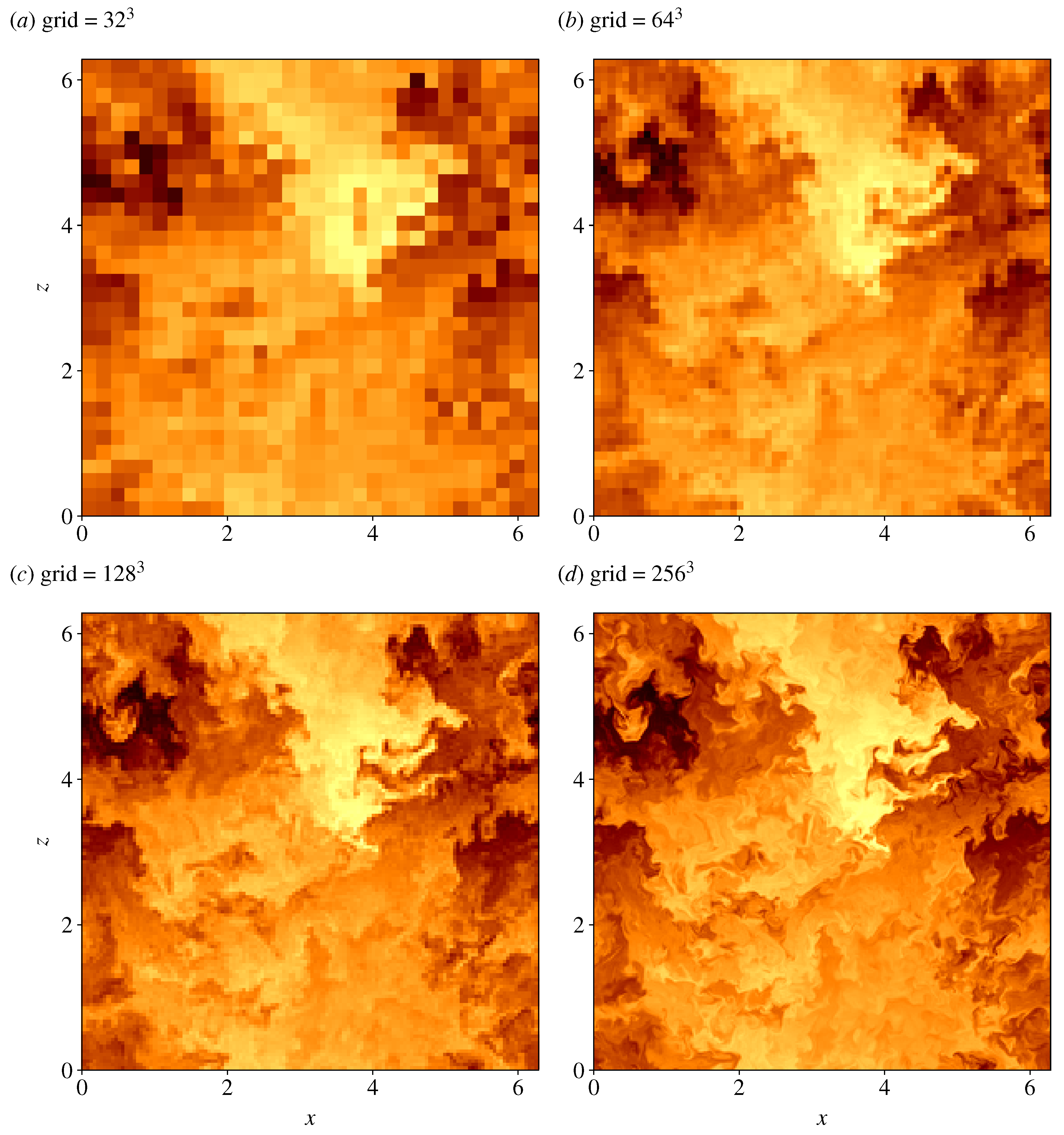
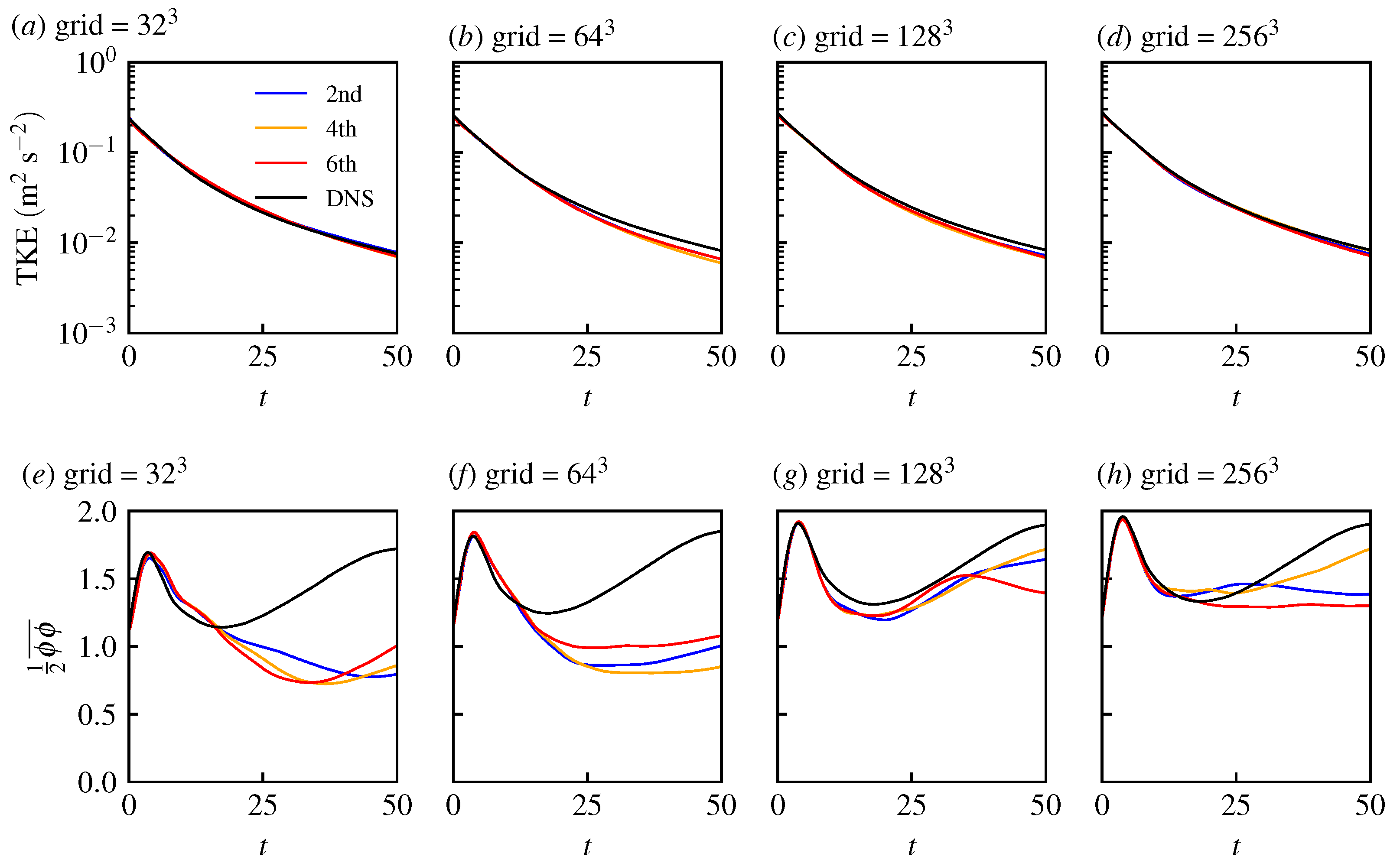
3.1. Homogeneous Isotropic Turbulence

Figure 3 show the comparison between HIT DNS and LES. Results from 12 LES runs (combinations of four grid resolutions and three SGS discretization orders of accuracy) are compared to the reference DNS results. TKE and scalar variance include only the resolved-scale flow; thus, the DNS curves slightly vary as the resolution changes. The LES and DNS agree well with respect to TKE. Some minor differences between the LES and DNS TKE are exaggerated because of the logarithmic y-axis in Figure 3. The LES TKE results are identical with respect to the SGS model discretization.

The evolution of scalar variance is different between LES and DNS for $t>10$, or about 5 times the large-scale turnover time based on the initial condition. For short times, the LES scalar variance agrees well with the DNS for all discretization orders of accuracy. The production of scalar variance depends on the turbulent structure, and as the flow evolves, the scalar LES turbulence production is different. Higher-resolution simulations, ${128}^3$ and ${256}^3$, have finer structures (Figure 1) and the LES scalar variance somewhat better follows the DNS results. Variance time traces show no trend with respect to the order of accuracy, which is the key result of the scalar variance results of Figure 3. The insensitivity of the results with respect to TKE is perhaps expected as the SGS model is essentially “exact” for HIT. However, the passive scalar field is not isotropic and presents a more challenging flow, potentially allowing the formation of scalar variance trends with respect to the discretization order.

Overall, the comparison between LES and DNS provides verification of the SGS model implementation for all orders of accuracy.

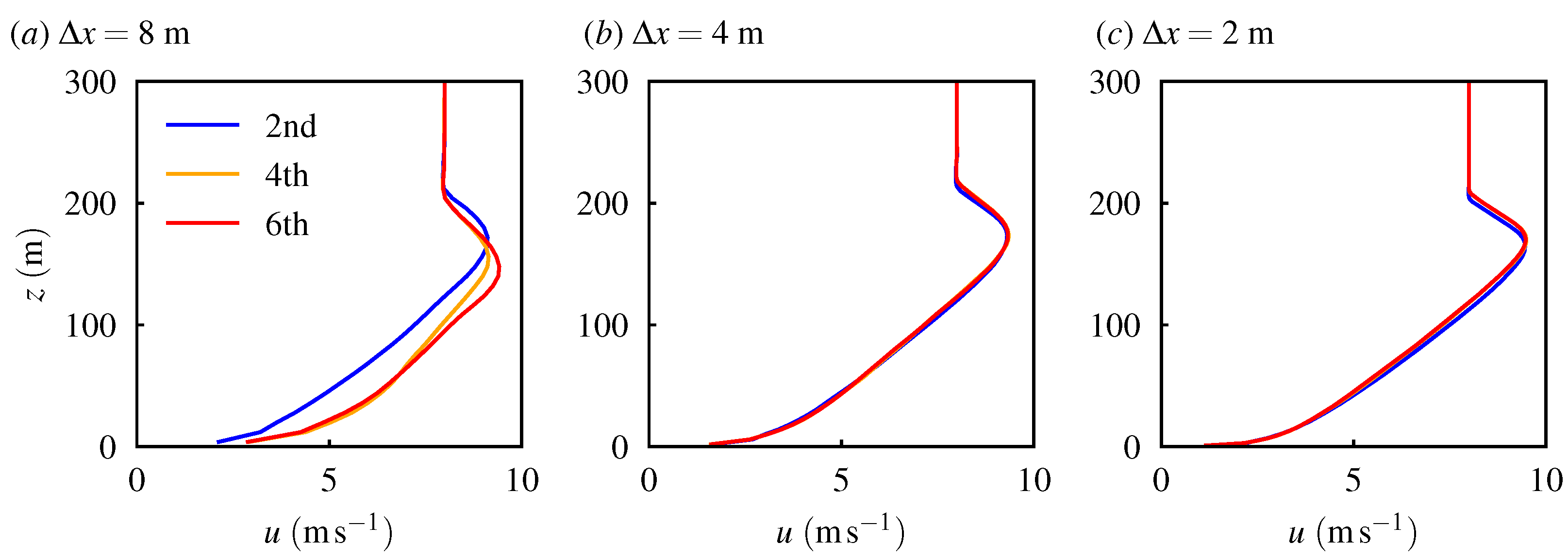
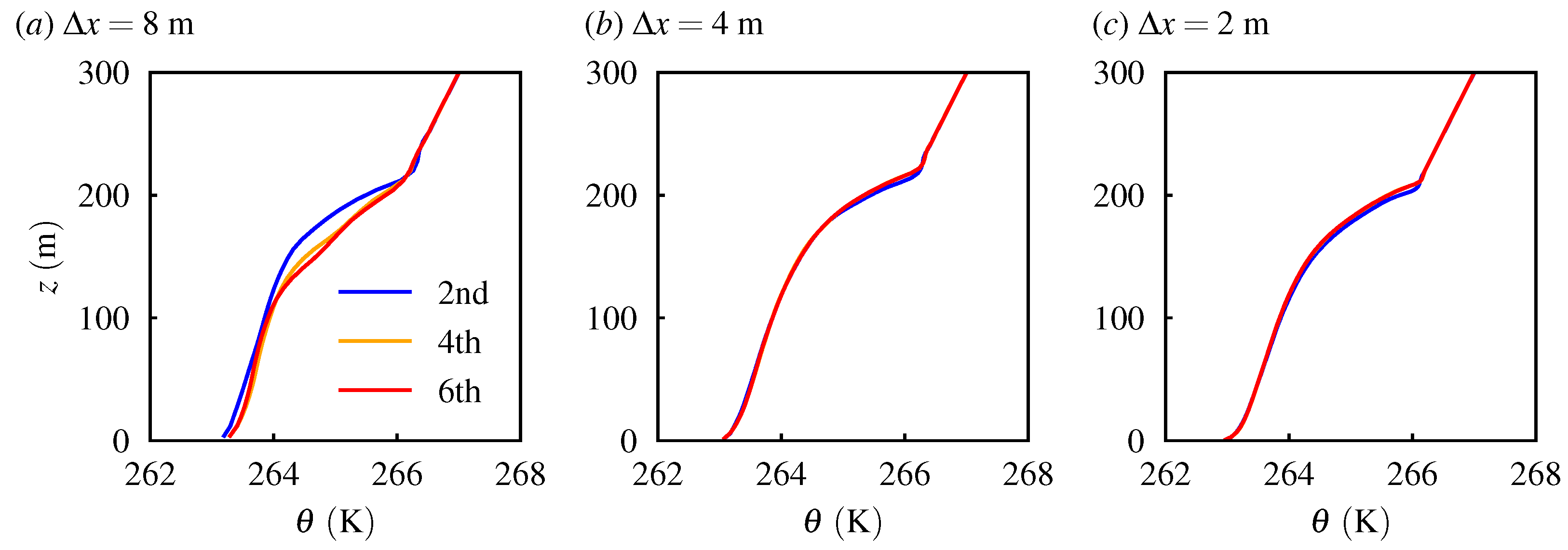
3.2. Stable Atmospheric Boundary Layer

The combination of mean shear and stable stratification results in a challenging flow for the SGS model. Mean shear breaks the assumption of isotropic SGS flow. Further, stable stratification confines the overturning flow scale, decreasing the range of scales of classical Kolmogorov turbulence [20,32]. Figure 4, Figure 5 and Figure 6 show profiles at $t=9\mathrm{h}$ of zonal velocity, potential temperature, and potential temperature flux. The temperature flux includes the SGS component. The boundary layer attains a statistically stationary state after $t>8\mathrm{h}$. Profiles are instantaneous horizontal averages.

Results differ with respect to the SGS discretization at the lowest grid resolution $\Delta x=8\mathrm{m}$, whereas the profiles at the other two finer resolutions are essentially identical. For $\Delta x=8\mathrm{m}$, about $90\%$ of TKE is resolved [4] and the depth of the boundary layer is resolved with 25 model levels. The simulation profiles with $\Delta x=4$ and $2\mathrm{m}$ agree well with the results of other models [4,10,21,33]. Only the second-order scheme yields accurate results for $\Delta x=8\mathrm{m}$.

The temperature flux exhibits large differences with respect to the SGS discretization. Figure 7 shows the time evolution of the resolved-scaled vertically integrated TKE, $\mathrm{VTKE}\left(t\right)={\displaystyle \frac{1}{2}}{\rho }_0\int (\langle u^{\prime }{u}^{\prime }\rangle +\langle v^{\prime }{v}^{\prime }\rangle +\langle w^{\prime }{w}^{\prime }\rangle )\mathrm{d}z$. The VTKE results show that the turbulence in the boundary layer erroneously collapses, that is, velocity fluctuations in the boundary layer are suppressed, similar to the results of [10]. The spurious collapse causes large variations in the turbulent fluxes (Figure 6), including the surface fluxes.

Turbulent flow spectra are used to help assess the impact of the discretization on the energy distribution across flow scales. Figure 8 and Figure 9 show one-dimensional spectra of zonal wind u along the x-direction for runs with $\Delta x=8\mathrm{m}$ (Figure 8) and $\Delta x=4\mathrm{m}$ (Figure 9) at the end of the simulation $t=9\mathrm{h}$. The spectra are normalized with the u covariance, which means that the integral under each curve is the same. This removes the difference in the turbulent flow between runs and at different heights, while retaining the difference in the energy distribution with respect to length scale. Because most of the differences are in the small scales (high wavenumbers), the spectra are premultiplied by $k^{5/3}$. Spectra for variables other than u and spectra along the y direction show the same qualitative behavior as the spectra in Figure 8 and Figure 9; thus, they are not shown here and the discussion of the figures is generalized to all variables and both x and y directions. Moreover, spectra for the $\Delta x=2\mathrm{m}$ runs have negligible differences with respect to the discretization order and are not plotted here.

Most of the differences in the spectra are observed near the surface. This is a challenging modeling component of this type of flow because the mean shear is stronger and the influence of the SGS model and unresolved flow is the highest; for instance, see SGS TKE profiles in [4]. In Figure 8 and Figure 9, spectra are plotted at four heights $z=0.5\Delta z$, $3.5\Delta z$, $7.5\Delta z$, and $15.5\Delta z$, which corresponds to model half-levels 1, 4, 8, and 16. The grid resolution is different between the two runs shown Figure 8 and Figure 9; thus, the physical heights of the spectra differ by a factor of 2 between the corresponding panels.

The spectra for runs using the second-order scheme differ with respect to the fourth- and sixth-order schemes. The differences are larger closer to the surface and are mostly observed at the small scales. Differences in spectral energy distribution near the grid scale are expected since these are the scales directly affected by the SGS model. The second-order scheme results in more energy at the small scales. The difference in energy is nearly a factor of ten very close to the surface, with the difference diminishing by the 16th model level (panel d in Figure 8 and Figure 9). In other words, the fourth- and sixth-order schemes dissipate more energy near the grid scale, which might help explain the better performance of the second-order scheme with respect to the mean profiles, turbulent heat flux, and TKE. The spectra are consistent with the results shown in Figure 7 as the differences between the three discretizations diminish when the turbulent flow is better resolved. This occurs in the spectra in two ways: as the height increases and as the grid resolution increases.

4. Conclusions

The effects of the Smagorinsky–Lilly subgrid scale (SGS) model discretization are investigated using three finite difference schemes. Second-, fourth-, and sixth-order centered difference schemes are used to approximate the spatial derivatives of the SGS model. The LES of two flows is carried out: decaying homogeneous isotropic turbulence (HIT), including (non-isotropic) turbulent mixing of a passive scalar, and a moderately stable atmospheric boundary layer. A direct numerical simulation of HIT with an initial Taylor Reynolds number of $R{e}_{\lambda }=230$ is used to verify the SGS model discretization and provide a baseline for the LES results.

In the HIT LES, no differences are observed with respect to the SGS model discretization. In the LES of a moderately stable atmospheric boundary layer, LES results depend on the SGS discretization for coarse grid resolutions. The second-order scheme performs better at coarse resolutions compared to higher-order schemes in the stable boundary layer LES. The present results suggest that at coarse grid resolutions, the high-order approximation does not provide any additional benefit compared to the second-order scheme. This is because the coarse LES fields at coarse resolutions are not smooth and contain significant amount of fluctuations at the grid scale, as shown in Figure 1. The finite difference approximation assumes fields of sufficient (polynomial) smoothness, which might not be present in the LES. Previous studies sacrificed the order of accuracy to optimize other types of model errors in the LES [16]. In HIT, the lack of strong flow organization at small scales does not result in any negative effects from the use of a higher-order approximation. However, in coarse LES of stable boundary layers, higher-order SGS approximations lead to large errors.

The SGS model includes two parameters, the Smagorinsky constant $C_s$ and the turbulent Prandtl number $P{r}_t$. Standard values were used, but as shown in previous studies [10], both model parameters can affect the LES result. Therefore, the presently observed discrepancies can be modulated by different model constant values.

Overall, it is found that higher-order discretizations of the Smagorinsky–Lilly model do not result in any benefit compared to the second-order scheme. In LES with coarse grid resolutions, the second-order scheme can better approximate the local spatial gradients of the resolved-scale field, compared to high-order approximations, and was found to yield more accurate results.

References

1. Pope, S.B. Ten questions concerning the large-eddy simulation of turbulent flows. N. J. Phys. 2004, 6, 35. [Google Scholar] [CrossRef]
2. Wyngaard, J.C. Turbulence in the Atmosphere; Cambridge University Press: Cambridge, UK, 2010. [Google Scholar]
3. Sullivan, P.G.; Patton, E.G. The effect of mesh resolution on convective boundary layer statistics and structures generated by large-eddy simulation. J. Atmos. Sci. 2011, 68, 2395–2415. [Google Scholar] [CrossRef]
4. Matheou, G.; Chung, D. Large-eddy simulation of stratified turbulence. Part II: Application of the stretched-vortex model to the atmospheric boundary layer. J. Atmos. Sci. 2014, 71, 4439–4460. [Google Scholar] [CrossRef]
5. Smagorinsky, J. General Circulation Experiments with the Primitive Equations. I. The Basic Experiment. Mon. Weather Rev. 1963, 91, 99–164. [Google Scholar] [CrossRef]
6. Lilly, D.K. On the Application of the Eddy Viscosity Concept in the Inertial Sub-Range of Turbulence; National Center for Atmospheric Research: Boulder, CO, USA, 1966; Volume 123. [Google Scholar]
7. Lilly, D.K. The representation of small-scale turbulence in numerical simulation experiments. In Proceedings of the IBM Scientific Computing Symposium on Environmental Sciences, Yorktown Heights, NY, USA, 14–15 November 1966; pp. 195–210. [Google Scholar]
8. Lele, S.K. Compact finite difference schemes with spectral-like resolution. J. Comput. Phys. 1992, 103, 16–42. [Google Scholar] [CrossRef]
9. Lomax, H.; Pulliam, T.H.; Zingg, D.W. Fundamentals of Computational Fluid Dynamics; Scientific Computation; Springer: Berlin/Heidelberg, Germany, 2003. [Google Scholar]
10. Matheou, G. Numerical discretization and subgrid-scale model effects on large-eddy simulations of a stable boundary layer. Q. J. R. Meteorol. Soc. 2016, 142, 3050–3062. [Google Scholar] [CrossRef]
11. Leonard, A. Energy cascade in large-eddy simulations of turbulent fluid flows. Adv. Geophys. 1974, 18, 237–248. [Google Scholar]
12. Ghosal, S. An analysis of numerical errors in large-eddy simulations of turbulence. J. Comput. Phys. 1996, 125, 187–206. [Google Scholar] [CrossRef]
13. Vreman, B.; Geurts, B.; Kuerten, H. Comparison of numerical schemes in large-eddy simulation of the temporal mixing layer. Int. J. Numer. Methods Fluids 1996, 22, 297–311. [Google Scholar] [CrossRef]
14. Chow, F.K.; Moin, P. A further study of numerical errors in large-eddy simulations. J. Comput. Phys. 2003, 184, 366–380. [Google Scholar] [CrossRef]
15. Meyers, J.; Geurts, B.J.; Baelmans, M. Database analysis of errors in large-eddy simulation. Phys. Fluids 2003, 15, 2740–2755. [Google Scholar] [CrossRef]
16. Hill, D.J.; Pullin, D.I. Hybrid tuned center-difference-WENO method for large eddy simulations in the presence of strong shocks. J. Comput. Phys. 2004, 194, 435–450. [Google Scholar] [CrossRef]
17. Overholt, M.R.; Pope, S.B. Direct numerical simulation of a passive scalar with imposed mean gradient in isotropic turbulence. Phys. Fluids 1996, 8, 3128–3148. [Google Scholar] [CrossRef]
18. Perlman, E.; Burns, R.; Li, Y.; Meneveau, C. Data exploration of turbulence simulations using a database cluster. In Proceedings of the 2007 ACM/IEEE Conference on Supercomputing, Reno, NV, USA, 10–16 November 2007; pp. 1–11. [Google Scholar]
19. Li, Y.; Perlman, E.; Wan, M.; Yang, Y.; Meneveau, C.; Burns, R.; Chen, S.; Szalay, A.; Eyink, G. A public turbulence database cluster and applications to study Lagrangian evolution of velocity increments in turbulence. J. Turbul. 2008, 9, N31. [Google Scholar] [CrossRef]
20. Chung, D.; Matheou, G. Direct numerical simulation of stationary homogeneous stratified sheared turbulence. J. Fluid Mech. 2012, 696, 434–467. [Google Scholar] [CrossRef]
21. Beare, R.J.; MacVean, M.K.; Holtslag, A.A.M.; Cuxart, J.; Esau, I.; Golaz, J.C.; Jimenez, M.A.; Khairoutdinov, M.; Kosovic, B.; Lewellen, D.; et al. An intercomparison of large-eddy simulations of the stable boundary layer. Bound.-Layer Meteorol. 2006, 118, 247–272. [Google Scholar] [CrossRef]
22. Batchelor, G.K. The condition for dynamical similarity of motions of a frictionless perfect-gas atmosphere. Q. J. R. Meteorol. Soc. 1953, 79, 224–235. [Google Scholar] [CrossRef]
23. Ogura, Y.; Phillips, N.A. Scale analysis of deep and shallow convection in the atmosphere. J. Atmos. Sci. 1962, 19, 173–179. [Google Scholar] [CrossRef]
24. Morinishi, Y.; Lund, T.S.; Vasilyev, O.V.; Moin, P. Fully Conservative Higher Order Finite Difference Schemes for Incompressible Flow. J. Comput. Phys. 1998, 143, 90–124. [Google Scholar] [CrossRef]
25. Spalart, P.R.; Moser, R.D.; Rogers, M.M. Spectral methods for the Navier–Stokes equations with one infinite and two periodic directions. J. Comput. Phys. 1991, 96, 297–324. [Google Scholar] [CrossRef]
26. Mason, P.J.; Callen, N.S. On the magnitude of the subgrid-scale eddy coefficient in large-eddy simulations of turbulent channel flow. J. Fluid Mech. 1986, 162, 439–462. [Google Scholar] [CrossRef]
27. Lilly, D.K. On the numerical simulation of buoyant convection. Tellus 1962, 14, 148–172. [Google Scholar] [CrossRef]
28. Canuto, V.M.; Cheng, Y. Determination of the Smagorinsky–Lilly constant CS. Phys. Fluids 1997, 9, 1368–1378. [Google Scholar] [CrossRef]
29. Harlow, F.H.; Welch, J.E. Numerical calculation of time-dependent viscous incompressible flow of fluid with free surface. Phys. Fluids 1965, 8, 2182–2189. [Google Scholar] [CrossRef]
30. Arakawa, A.; Lamb, V.R. Computational design of the basic dynamical processes of the UCLA general circulation model. In Methods of Computational Physics; Academic Press: Cambridge, MA, USA, 1977; Volume 17, pp. 173–265. [Google Scholar]
31. Matheou, G.; Chung, D.; Nuijens, L.; Stevens, B.; Teixeira, J. On the fidelity of large-eddy simulation of shallow precipitating cumulus convection. Mon. Weather Rev. 2011, 139, 2918–2939. [Google Scholar] [CrossRef]
32. Kaimal, J.C.; Wyngaard, J.C.; Izumi, Y.; Coté, O.R. Spectral characteristics of surface-layer turbulence. Q. J. R. Meteorol. Soc. 1972, 98, 563–589. [Google Scholar]
33. Sullivan, P.P.; Weil, J.C.; Patton, E.G.; Jonker, H.J.; Mironov, D.V. Turbulent winds and temperature fronts in large-eddy simulations of the stable atmospheric boundary layer. J. Atmos. Sci. 2016, 73, 1815–1840. [Google Scholar] [CrossRef]
Figure 1. Vertical planes of the LES initial scalar fluctuations fields. The LES initial condition is constructed using coarsened DNS data. The panels show four LES grid resolutions: (a) 32 3 grid, (b) 64 3 grid, (c) 128 3 grid, and (d) 256 3 grid. The DNS grid size is 1024 3 , which is 4 times finer than the field in panel (d).
Atmosphere 16 00310 g001
Figure 2. LES model grid configuration. A three-dimensional grid cell schematic is shown on the left. The corresponding two-dimensional configuration is shown on the right. Scalar variables and the diagonal elements of the stress tensor τ are located at the grid cell centers. The velocity components (u, v, and w) and components of the SGS scalar flux ( σ ) are located at the middle of the cell faces. The off-diagonal elements of the stress tensor are located at the middle grid cell edges in three dimensions (left) and at the grid cell corners in two dimensions (right).
Atmosphere 16 00310 g002
Figure 3. Comparison of resolved-scale TKE and scalar variance between the DNS and LES. (Top row) Panels (ad) correspond to TKE and (bottom row) (eh) correspond to scalar variance. Each column corresponds to a different LES grid resolution: (a,e) 32 3 grid, (b,f) 64 3 grid, (c,g) 128 3 grid, and (d,h) 256 3 grid.
Atmosphere 16 00310 g003
Figure 4. Stable boundary layer zonal velocity profiles at different LES grid resolutions and SGS term discretizations at t = 9 h . Each panel corresponds to a different grid resolution. Lines correspond to different orders of SGS term discretizations.
Atmosphere 16 00310 g004
Figure 5. Stable boundary layer potential temperature profiles at different LES grid resolutions and SGS term discretizations at t = 9 h . Each panel corresponds to a different grid resolution: (a) Δ x = 8 m , (b) Δ x = 4 m , and (c) Δ x = 2 m . Lines correspond to different orders of SGS term discretization.
Atmosphere 16 00310 g005
Figure 6. Stable boundary layer turbulent heat flux at different LES grid resolutions and SGS term discretizations at t = 9 h . Each panel corresponds to a different grid resolution: (a) Δ x = 8 m , (b) Δ x = 4 m , and (c) Δ x = 2 m . Lines correspond to different orders of SGS term discretization.
Atmosphere 16 00310 g006
Figure 7. Stable boundary layer time traces of vertically integrated TKE at different LES grid resolutions and SGS term discretizations. Each panel corresponds to a different grid resolution: (a) Δ x = 8 m , (b) Δ x = 4 m , and (c) Δ x = 2 m . Lines correspond to different orders of SGS term discretization.
Atmosphere 16 00310 g007
Figure 8. One-dimensional compensated spectra of zonal wind for the stable boundary layer at grid resolution Δ x = 8 m at t = 9 h . Each panel corresponds to a different height. Color lines correspond to different orders of the SGS term discretization, as in Figure 7. Black line denotes slope k 1 for reference.
Atmosphere 16 00310 g008
Figure 9. One-dimensional compensated spectra of zonal wind for the stable boundary layer at grid resolution Δ x = 4 m at t = 9 h . Each panel corresponds to a different height. Color lines correspond to different orders of the SGS term discretization, as in Figure 7. Black line denotes slope k 1 for reference.
Atmosphere 16 00310 g009