Article

Assessing the Impact of Climatic Factors and Air Pollutants on Cardiovascular Mortality in the Eastern Mediterranean Using Machine Learning Models

by
Kyriaki Psistaki
1,†,
Damhan Richardson
2,†,
Souzana Achilleos
3,
Mark Roantree
4 and
Anastasia K. Paschalidou
1,*
1
Department of Forestry and Management of the Environment and Natural Resources, Democritus University of Thrace, 68200 Orestiada, Greece
2
Insight Centre for Data Analytics, Dublin City University, D09 V209 Dublin, Ireland
3
Department of Primary Care and Population Health, University of Nicosia Medical School, 2414 Nicosia, Cyprus
4
School of Computing, Dublin City University, D09 V209 Dublin, Ireland
*
Author to whom correspondence should be addressed.
These authors contributed equally to this work.
Atmosphere 2025, 16(3), 325; https://doi.org/10.3390/atmos16030325
Submission received: 29 January 2025 / Revised: 5 March 2025 / Accepted: 9 March 2025 / Published: 12 March 2025

Abstract

:
Cardiovascular diseases are the most common cause of death worldwide, with atmospheric pollution, and primarily particulate matter, standing out as the most hazardous environmental factor. To explore the exposure–response curves, traditional epidemiological studies rely on generalised additive or linear models and numerous works have demonstrated the relative risk and the attributable fraction of mortality/morbidity associated with exposure to increased levels of particulate matter. An alternative, probably more effective, procedure to address the above issue is using machine learning models, which are flexible and often outperform traditional methods due to their ability to handle both structured and unstructured data, as well as having the capacity to capture non-linear, complex associations and interactions between multiple variables. This study uses five advanced machine learning techniques to examine the contribution of several climatic factors and air pollutants to cardiovascular mortality in the Eastern Mediterranean region, focusing on Thessaloniki, Greece, and Limassol, Cyprus, covering the periods 1999–2016 and 2005–2019, respectively. Our findings highlight that temperature fluctuations and major air pollutants significantly affect cardiovascular mortality and confirm the higher health impact of temperature and finer particles. The lag analysis performed suggests a delayed effect of temperature and air pollution, showing a temporal delay in health effects following exposure to air pollution and climatic fluctuations, while the seasonal analysis suggests that environmental factors may explain greater variability in cardiovascular mortality during the warm season. Overall, it was concluded that both air quality improvements and adaptive measures to temperature extremes are critical for mitigating cardiovascular risks in the Eastern Mediterranean.

1. Introduction

Cardiovascular diseases (CVDs), primarily ischemic heart disease and stroke, are the most common cause of death worldwide, accounting for more than 30% of annual global mortality [1]. It is noteworthy that in 2019, 18.5 million deaths globally were attributed to CVDs, 33% of which occurred among adults between 30 and 70 years old [2]. Although global CVD death rates have followed a descending trend over the past three decades, in recent years this reduction has slowed down, or even reversed in many regions, highlighting the need to enhance prevention measures [1,2,3].
Among the leading risk factors for CVD morbidity and mortality, air pollution stands out as the most hazardous environmental factor [4]. A large body of literature has associated both short- and long-term exposure to air pollution with increased mortality from a wide range of causes, e.g., refs. [5,6,7,8,9,10,11]. In urban environments, where air pollution levels are typically high, traffic-related emissions can lead to respiratory diseases (e.g., respiratory tuberculosis, malignant neoplasm of the trachea, bronchus, and lung, pneumonia, chronic lower respiratory diseases, and other acute lower respiratory infections), and CVD and cerebrovascular diseases (e.g., ischemic heart diseases, pulmonary embolism, cerebrovascular diseases), as well as metabolic disorders such as diabetes mellitus [12]. Overall, the severity of adverse outcomes depends on various factors, including individual characteristics, such as age, preexisting health conditions, body mass index, sex, smoking status, and socio-economic background, the nature of the atmospheric pollutant, as well as the duration and dose of exposure [8].
One of the most harmful atmospheric pollutants is particulate matter with an aerodynamic diameter of ≤2.5 μm (PM2.5), which ranks among the five most critical health risk factors globally [13]. Over the past thirty years, the impact of ambient PM2.5 on the burden of CVD has grown, causing 2.48 million premature deaths and a loss of 60.91 million healthy life-years due to CVD-related premature mortality, diseases, and disabilities (disability-adjusted life years (DALYs)) globally in 2019 [14]. Despite international agencies, such as the World Health Organization (WHO), having recommended guidelines for air pollution levels, and many regions worldwide having implemented legislation to improve air quality, e.g., refs. [15,16], approximately 99% of the global population is exposed to levels above the WHO recommendations, particularly in low- and middle-income countries [17].
In addition to air pollution, temperatures exceeding human thermal comfort limits, referred to as non-optimum temperatures, represent another important environmental risk factor for CVD mortality [4]. Although humans can adapt to their thermal environment through cultural, behavioural, and physiological mechanisms, exposure to non-optimum temperatures can strain the cardiovascular system [18]. In 2021, non-optimum temperatures were responsible for 1.17 million CVD deaths globally, with the heat-related impacts being particularly severe in Eastern Europe and the cold-related impacts dominating in sub-Saharan Africa [4]. Given the threats posed by a constantly warming climate, the devastating health impacts of high temperatures and heatwaves have been well established [19,20]. In this context, and considering that urban populations experience higher temperatures than those living in non-urban areas due to the urban heat island phenomenon, some studies have compared heat-related effects between urban and non-urban areas. However, the findings remain inconsistent. While there is evidence that high urbanisation levels are associated with increased risk of mortality, according to some studies, populations in suburban areas are more vulnerable to heat effects, highlighting differences in air conditioning usage, healthcare access, socioeconomic status, and population age distribution as possible determinants [21].
Furthermore, along with temperature, other meteorological parameters, such as humidity and wind speed, also affect thermal comfort [22,23,24] and potentially human health. Evidence suggests that these meteorological parameters, either individually or in combination with temperature, can increase the CVD risk and mortality [25,26,27,28].
Traditionally, epidemiological studies aiming to explore the acute impact of thermal stress and air pollution on public health have applied regression models to provide estimates of the relative risk and burden of mortality, e.g., refs. [5,11,29,30,31,32,33,34,35,36,37]. On the other hand, several studies have used machine learning (ML) to investigate the health impacts of environmental factors, and specifically to identify key predictors of mortality or morbidity, and sometimes to evaluate the most effective models for describing exposure-response relationships, e.g., refs. [38,39,40,41,42,43,44,45,46]. The advantages of the latter approach are that ML models are flexible and often outperform traditional methods due to their ability to handle both structured and unstructured data, as well as their capacity to capture non-linear, complex associations and interactions between multiple variables. Results provided by this kind of study can help local authorities and healthcare professionals to develop effective prevention strategies, improve early warning systems, and reduce the impact of environmental factors and climate change on public health and the economy.
Climate change is expected to exacerbate the health risks associated with air pollution and non-optimum temperatures in the future. By the end of the century, mortality attributed to air pollution is projected to increase approximately fivefold globally, from 4061 (95% CI: 2493–6188) thousand in 2000 to 19,539 (95% CI: 11,373–31,280) thousand in 2090, according to the medium climate scenario SSP2-4.5. Similarly, mortality due to non-optimum temperature is projected to increase approximately sevenfold, from 1593 (95% CI: 582–2832) thousand in 2000 to 10,777 (95% CI: 2223–21,845) thousand in 2090 [47]. However, considering the potential synergistic effects between air pollution and temperature, the overall health impact could be even greater. Although inconsistent among different studies, there is evidence suggesting that high levels of air pollution can exacerbate temperature-related health effects, particularly those associated with heat exposure [48,49,50,51,52].
The Eastern Mediterranean (EM) region is a prominent climate change hotspot, experiencing a pronounced decline in precipitation and high warming rates that exceed the global average, particularly during the summer [53,54]. Projections indicate that these trends are expected to persist throughout the century, along with a substantial increase in the duration, frequency, and intensity of heatwaves [54,55]. Additionally, the EM, located at the crossroads of three continents, is affected by air pollution emissions from continental Europe and Asia, as well as dust storms from the African and Arabian deserts. Furthermore, its geographic location along with its climate, which promotes the formation of secondary pollutants through photochemical processes, favours the accumulation of air pollution, and often results in poor air quality [56,57].
Previous studies in the region have demonstrated the adverse impact of air pollution and thermal stress, separately, on public health through using time-series approaches [29,34,35,36,37,58,59]. However, non-linear, complex associations and interactions between multiple variables usually strain traditional studies. To overcome such shortcomings, this study uses ML models to identify the best-performing model for predicting CVD mortality and the most influential environmental factors on CVD mortality in two typical EM environments: Thessaloniki, in Northern Greece; and Limassol, in Cyprus (Figure 1). In order to ensure that a sufficiently robust study is conducted, we adopt a similar approach to [60], where a range of ML functions are evaluated using multiple metrics together with a feature importance study. To the best of our knowledge, this is the first study to address these issues in Greece and Cyprus. It is expected that this analysis can improve forecasting methods in epidemiological research and may become the basis for future, even more detailed, studies, with the inclusion of additional social and demographic factors.

2. Materials and Methods

2.1. Data Collection

Daily cardiovascular (ICD10 I00-I99) mortality data were collected from two sources: the Hellenic Statistical Authority in Greece, covering the period from January 1999 to December 2016; and the Health Monitoring Unit of the Ministry of Health in Cyprus, from January 2005 to December 2019. The mortality data focused on residents of Thessaloniki and Limassol, respectively. Environmental data on air pollutant concentrations were obtained from the Atmospheric Pollution Control Stations of the Municipality of Thessaloniki in Greece, and the Air Quality and Strategic Planning Section, Department of Labour Inspection, Ministry of Labour and Social Insurance in Cyprus. In Thessaloniki, the data were collected from three stations (two urban-traffic stations and one urban-background station) and were averaged across the three stations (Figure S1, Table S1). These stations provided daily averages of particulates (PM2.5, in μg/m3, and particulate matter with diameter ≤ 10 μm, PM10, in μg/m3), as well as hourly measurements of ozone (O3, in μg/m3), sulphur dioxide (SO2, in μg/m3), nitrogen oxide (NO, in μg/m3), nitrogen dioxide (NO2, in μg/m3), and carbon monoxide (CO, in μg/m3). In Limassol, data for the same pollutants were collected from one urban-traffic station, with PM2.5 data sourced from a residential station (Figure S1, Table S1). For both locations, 24 h average pollutant concentrations were calculated for days with at least 12 hourly observations. PM10 data were available for the entire study period for each city. However, PM2.5 data availability varied, with Thessaloniki’s records beginning on 30 June 2004 and Limassol’s records beginning on 8 January 2009. Meteorological data, including daily mean temperature (Temp, in °C)) and relative humidity (RH, in %), were obtained from the Municipality of Thessaloniki and the Cyprus Department of Meteorology (Table S1). The dataset for Thessaloniki also contained wind speed values (ws, in m/s). It is noted that ws values were not used for Limassol due to low temporal coverage. A full description of the data and data manipulation can be found in Psistaki et al. [35], and summary statistics of the variables can be found in Table S2.

2.2. Feature Selection

The analyses were performed on trimmed versions of the datasets in order to mitigate the effect of outliers, i.e., the highest and lowest 5% of PM2.5 and PM10 data were excluded symmetrically from both tails of the distribution to avoid the effect of outlying values on the estimates [30]. The Pearson correlation coefficient (r) was calculated pairwise for each variable in the feature sets and interpreted based on the following threshold: values greater than 0.8 (r > 0.8) were considered to be a very strong positive correlation and values of r < −0.8 were classified as a very strong negative correlation.
NO2 and NO had a very strong correlation (0.82), and so NO2 was chosen to remain due to it having a lower correlation with O3 (0.76) compared to NO with O3 (0.86). The very strong correlation between PM10 and PM2.5 (0.83) was the motivation behind having separate models for both PM10 and PM2.5. In the end, 10 variables (i.e., temp, RH, ws, PM2.5/PM10, O3, NO2, SO2, CO, year, weekday) were used to explain the daily CVD mortality in Thessaloniki, using data across 3937 days for the PM2.5 model and 5137 days for the PM10 model, respectively. Similarly, CVD mortality in Limassol was explained using 9 variables (i.e., temp, RH, PM2.5/PM10, O3, NO2, SO2, CO, year, weekday) across 3184 days for the PM2.5 model and 3920 days for the PM10 model.

2.3. CVD Mortality Modelling

To develop predictive models for daily cardiovascular mortality in Thessaloniki and Limassol, five different tree-based ML models were used, namely, DecisionTreeRegressor (DT), along with the ensemble tree-based learners RandomForestRegressor (RF), ExtraTreesRegressor (ET), and AdaBoostRegressor (AB) from the scikit-learn python ML library [61], and XGBRegressor from the XGBoost library [62]. Ensemble learning, used in the latter four models, is an ML technique where multiple models are combined to improve the predictive performance of the overall model. Each of the four ensemble models combined multiple decision trees in different ways and as a result gained increased robustness against noisy data and outliers, improved predictive accuracy, and better generalisation. For the ML models employed in this study, it was not necessary to normalise the input variables, as this process was previously shown in [63,64] to have little effect on overall predictive performance. This decision is further supported by our discussion on the importance of variables, where those with higher ranges demonstrated no noticeable advantage. Ten-fold cross-validation was used on a rolling basis to preserve the temporal order of the data due to its time-series nature. Cross-validation is a commonly used method in ML, used ‘to assess the generalisation ability of a predictive model and to prevent overfitting’ [65]. In 10-fold cross-validation, the data are split into 10 subsets, each known as a ‘fold’. The model is then trained and tested in 10 iterations, alternating which folds are used for training and which for testing the model. After completing all 10 iterations, the performance metrics for each iteration are averaged to provide a more reliable measure of the way in which the model generalises to new data. In the context of our study, 10-fold cross-validation was implemented using the TimeSeriesSplit function from scikit-learn [61]. This function is a specialised cross-validation method suitable for time-series data, as it ensures that the temporal ordering of observations is preserved. This maintains the sequential nature of the data, by only predicting future data using past data.
Initially, forecasts were conducted on the original data and then the predictions were repeated on data where the PM10 and PM2.5 features were lagged, across lags of 1, 2, and 3 days. Given four lag intervals (0–3 days) and two particulate matter granularities (2.5 and 10), this produced 8 datasets for each city. Training the aforementioned models on each of these datasets resulted in a total of 40 sets of results for each city. This approach was undertaken to investigate the potential impact of delayed effects of particulate matter exposure on the prediction of mortality rates.
Our study also examined the impact of seasonality, developing distinct models for the warm (May to October) and cold (November to April) months using a lag of 0 days. This facilitated a comparative analysis of the predictive performance previously discussed along with an examination of how seasonality influenced feature importance, as discussed below. The four datasets derived for each city were used to train the five aforementioned models, resulting in 20 sets of results for each city. It is noted that our seasonal analysis was restricted to a lag of 0 days to provide some insight into the way seasonality influences feature importance and the predictive performance of our model. In order to keep our results and discussion concise, we chose to omit the full 0-to-3-day lag analysis.

2.4. Evaluation Metrics and Feature Importance

In this study, two quantitative evaluation metrics were used to facilitate comparative analysis across models and across different lag intervals: mean absolute error (MAE), and root mean squared error (RMSE). For each city, the model which had the smallest cross-validated RMSE and MAE scores was chosen as the ‘best performing’ model.
While determining optimal predictive performance is a general goal of ML, understanding which variables are important in predicting the outcome is also necessary for a greater understanding. Feature importance produces a score which enables the ranking of features from largest to smallest contribution to the model’s overall predictive power. Some of the ML models used in this study such as RF have been shown in the past to suffer significantly from the presence of superfluous features [66]. Alternatively, the discovery of highly relevant features is equally important, enabling a drill down in terms of a model’s interpretability. In our study, the best-performing model for each city was used for feature importance analysis. These metrics were computed and subsequently normalised so that their total sum was equal to one. They were then plotted using matplotlib, a python library used for visualisations [67]. Plotting each feature’s importance allows for an easier indication of the scale of difference in importance between each feature. For this study, the feature importance was examined for each lag, each particulate matter granularity, and for each of our seasonal models.

3. Results

3.1. Comparison of PM2.5 and PM10 Models Across Lags

Table 1 and Table 2 present the performance metrics for Thessaloniki and Limassol across PM2.5 and PM10, from zero to three lag days, for each of the different ML models.
For Thessaloniki, both the PM2.5 and PM10 models obtained the best performance with the AB model. Limassol found the best performance under the RF model. For both cities, this was the case for both MAE and RMSE values. AB for Thessaloniki and RF for Limassol generally had lower RMSE values for their PM2.5 models compared to their PM10 models, with a limited number of exceptions. The same held true for MAE, where the PM2.5 models generally exhibited lower MAE values than their respective PM10 models, with a limited number of exceptions.
When considering RMSE scores across each of the lags, Thessaloniki’s AB model had the best RMSE at a 3-day lag for PM2.5 and a 2-day lag for PM10. Similarly, Limassol’s RF model had the best RMSE at a 3-day lag for PM2.5 and at a 2-day lag for PM10.

3.2. Seasonal Analysis of Model Performance

Table 3 and Table 4 present the performance metrics for Thessaloniki and Limassol for models fitted separately for the warm and cold months at a lag of 0 days.
Congruent to the non-seasonal models, AB displayed the best performance for Thessaloniki for both the PM2.5- and PM10-trained models. Limassol saw RF as the best model again, but only during the warm season-trained models. The cold season PM2.5 and PM10 models instead performed better using the ET model. However, RF in the warm season models performed better than ET did for the cold season models. This trend of better performance from warm season models held true for both cities and both PM2.5- and PM10-trained models, with the limited exception of Limassol’s PM2.5 DT model.
When comparing seasonal models with mixed seasonal models, the warm season models in Thessaloniki performed better, while the cold season models performed worse than the mixed season models. The same held true for Limassol for both warm and cold season models. This can be seen in Table 3 and Table 4, where in the case of Thessaloniki, MAE was 5.7% lower for the PM2.5 warm model and 5.4% lower for its RMSE. The Thessaloniki PM10 model saw a 6.5% and 7.1% lower MAE and RMSE, respectively. The same can be seen in Limassol, where MAE and RMSE were 9.7% and 11.4% lower for its PM2.5 model and 13.5% and 14.8% for its PM10 model, respectively.

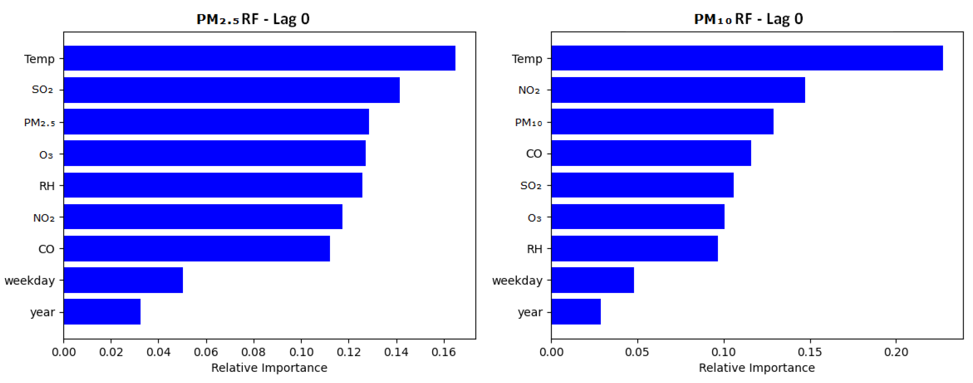
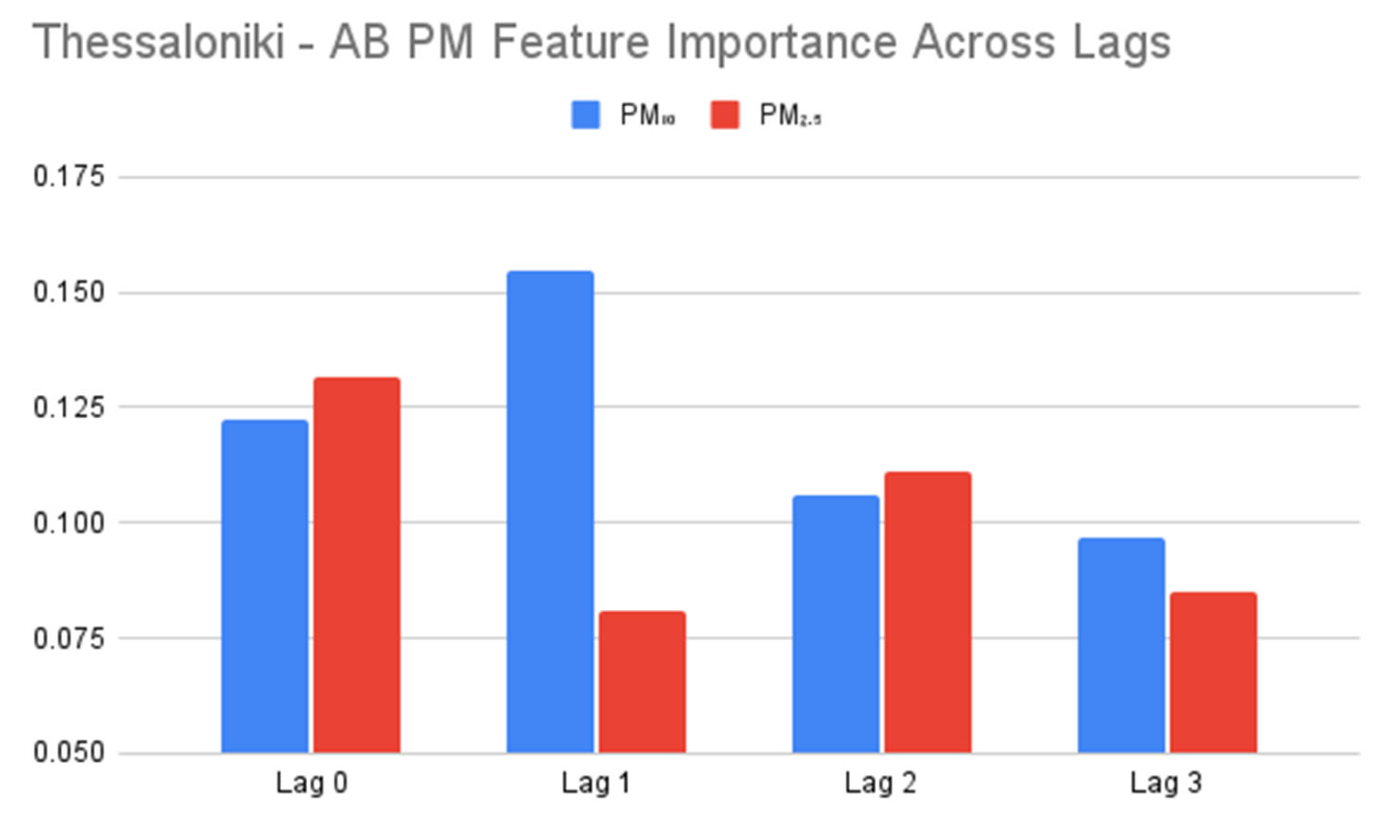
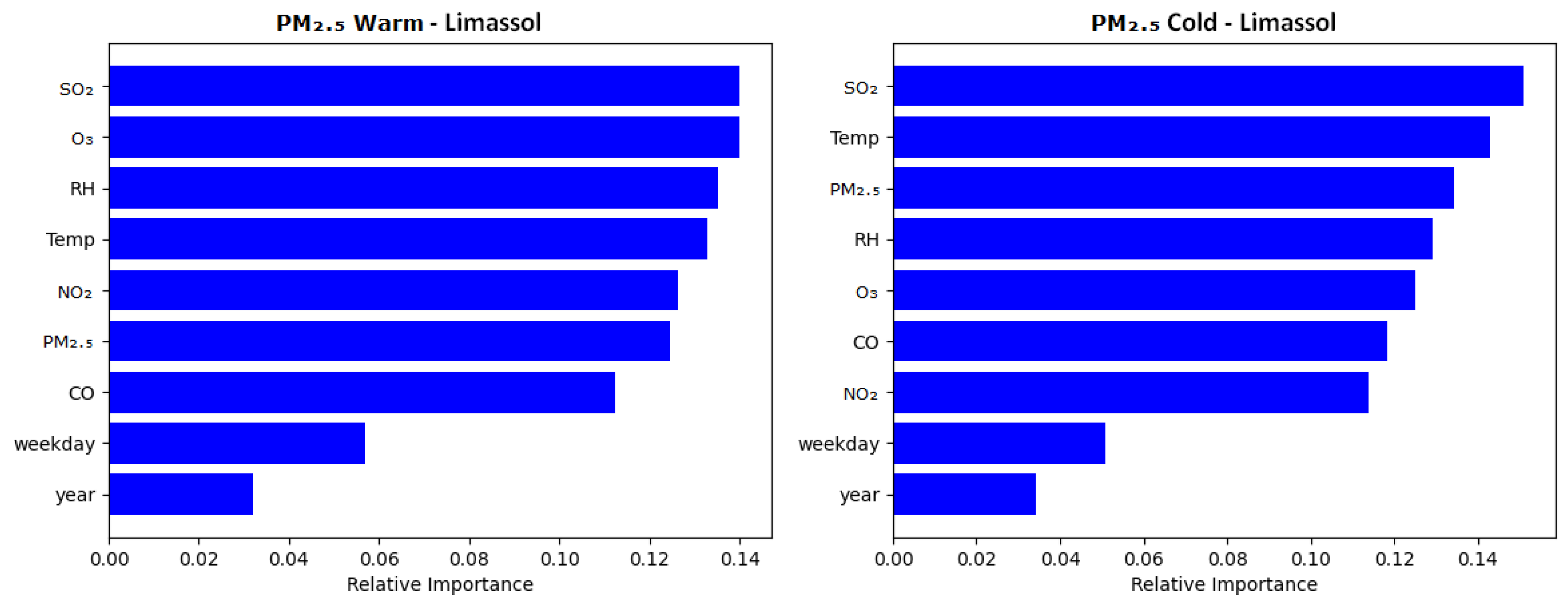
3.3. Feature Importance

3.3.1. Comparison Across Lags

In Figure 2 and Figure 3, the feature importance is compared across the PM2.5 and PM10 models at a lag of 0 for Thessaloniki and Limassol, respectively. Bar charts illustrating the change in importance of PM2.5 and PM10 as a feature across the increasing lags are shown in Figure 4 and Figure 5 for Thessaloniki and Limassol, respectively.
Temperature was the most important feature by a significant margin, for both particulate matter granularities for both cities. Temperature exceeded the remaining features in importance by a larger margin in Thessaloniki’s AB models compared to Limassol’s RF models.
The three most important features for each city were the same when separated by particulate matter granularity, despite each city having different best-performing models (AB in Thessaloniki and RF in Limassol). The PM2.5 models for both cities saw temperature, SO2, and PM2.5 as their most important features, while the PM10 models for both cities saw temperature, NO2, and PM10 as most important instead. The lowest individual relative importance was seen in the ‘weekday’ and ‘year’ variables, which yielded the lowest importance across every model in each city by a considerable margin. Specifically, in Figure 2 and Figure 3, weekday had a mean importance of 0.039 and year had a mean importance of 0.033, compared to the mean importance of features excluding weekday and year, which was 0.127.
The change in the particulate matter variable’s feature importance across lags varied by city. Thessaloniki’s AB models saw variable changes in feature importance across lags for PM2.5 and PM10. While PM2.5′s importance plummeted for a lag of 1 day and slightly recovered for the higher lags, PM10′s importance spiked at a lag of 1 day, before slowly tapering off for the remaining two lags.
Comparatively, Limassol’s RF models saw a minor change in the feature importance of PM2.5 or PM10 across lags. PM2.5 saw its highest importance at a lag of 1 day, but only slightly, whereas PM10 saw its highest importance at a lag of 2 days; however, this was an almost negligible increase. It is noted that although models may have performed better at longer lags, this was not necessarily always linked to a linear increase in their importance, as other predictive variables saw some greater importance at longer lags. The full variable set of importance graphs across lags are illustrated in Figures S2–S5.

3.3.2. Seasonality

Figure 6, Figure 7, Figure 8 and Figure 9 provide comparisons of feature importance for the seasonal models of Thessaloniki and Limassol.
The separation of the PM2.5 and PM10 models into distinct warm season and cold season variants resulted in seeing a large decrease in temperature’s relative importance as a predictor variable, in comparison to the mixed seasonal models. The PM2.5 and PM10 models for Thessaloniki, as well as the PM2.5 models for Limassol, demonstrated a heightened relative importance of their respective particulate matter variable in the cold season models compared to the warm season models, with the exception of Limassol’s PM10 model, which deviated from this trend. The lowest individual relative importance was seen in the ‘weekday’ and ‘year’ variables, which consistently yielded the lowest importance across every model in each city by a considerable margin. Specifically, in Figure 6, Figure 7, Figure 8 and Figure 9, weekday showed a mean importance of 0.044 and year had a mean importance of 0.031 compared to the remaining features’ mean of 0.123.

4. Discussion

The present study examined the contribution of several climatic factors and air pollutants to CVD mortality in the Eastern Mediterranean, focusing on Thessaloniki, Greece (1999–2016), and Limassol, Cyprus (2005–2019), using advanced ML models. Our findings highlighted that temperature fluctuations and major air pollutants, particularly SO2, NO2, and particulate matter, significantly affect CVD mortality.
In Thessaloniki, the AB model demonstrated the highest predictive performance, while RF performed best in Limassol, suggesting regional differences in data structure, pollutants, or other relevant city and population characteristics, such as information about the terrain, road networks, and emission sources, as well as age distribution, socioeconomic status, and exposure behaviours of the population. In atmospheric pollution research, ML is primarily used for source apportionment, air pollution forecasting/prediction, and estimating exposure for health studies, rather than directly estimating the effect of air pollution on health [68]. Therefore, comparing our model performance results with other studies using ML to assess the influence of environmental factors on CVD mortality was not feasible. However, in a study by Boudreault et al. [42], DT, RF, Gradient Boosting Machine (GBM), Single- and Multi-Layer Perceptrons (SLPs and MLPs) and Long Short-Term Memory (LSTM) were used to model the relationship between climatic variables and air pollutants’ all-cause mortality in Montreal. Overall, the ensemble tree-based models outperformed the neural networks, with the GBM showing the best performance. The Light Gradient Boosting Machine (LightGBM) was also found to perform better compared to the other five ML algorithms when applied to CVD admissions [40]. However, neural networks require significantly more data and are slower to build when compared to the models used in our study.
Our models trained on PM2.5 data generally outperformed those trained on PM10 data, supporting previous evidence on the greater health impact of finer particulate matter on CVD mortality and morbidity [8,69]. The best performance scores for both cities occurred at different lags, with peak performance at 2–3 lag days, suggesting a temporal delay in health effects following exposure to air pollution and climatic fluctuations. This aligns with previous studies showing a delayed effect of temperature and air pollution, with the strongest impact between a lag of 0 and 4 days [30,59,70]. However, while our models performed better at longer lags, this was not necessarily always linked to a linear increase in importance, as other predictive variables may have still performed better at longer lags.
Temperature consistently emerged as the most important predictor across all models, underscoring its central role in CVD mortality. Temperature was also found as the most important variable among climatic and air pollutants variables for all-cause mortality in Montreal, Canada [42], and in the USA [38], as well as for CVD admissions in Chengdu, China [40]. In addition, temperature, atmospheric pressure, and CO constitute the most influential factors for predicting CVD admissions in southern Italy [44,71]. Our findings are consistent with studies showing that exposure to extreme hot and cold temperatures is associated with a higher risk of mortality from cardiovascular conditions [72]. Extreme temperatures affect CVD mortality through various physiological mechanisms. Heat exposure causes increased skin blood flow and sweating, which can lead to volume depletion and sympathetic activation, increasing heart rate and risk of ischemia. Conversely, cold exposure induces vasoconstriction and increased blood pressure, which raises cardiac oxygen demand and can lead to plaque rupture and myocardial infarction, particularly in individuals with preexisting conditions.
Particles (PM2.5, PM10), SO2, and NO2 were also significant predictors, consistently appearing among the top predictors. An umbrella review by de Bont et al. [8] concluded that increased short-term exposure to PM2.5, PM10, and NOx was statistically significantly associated with CVD mortality. Moreover, a large multi-city study found that short-term exposure to SO2 was associated with an excess all-cause mortality fraction of 0.50% (95% empirical CI: 0.42%, 0.57%) [73]. Recent studies have highlighted several mechanisms through which air pollution impacts CVD, primarily involving oxidative stress, inflammation, autonomic imbalance, and particle translocation [8]. These mechanisms can trigger secondary pathways like endothelial dysfunction and epigenomic changes, contributing to CVD outcomes such as arrhythmias, increased blood pressure, and atherosclerosis. The specific pathways activated depend on the pollutant type, exposure dose, and duration, ultimately affecting risks for events like heart attacks and strokes.
On the other hand, the lowest individual relative importance was seen in the ‘weekday’ and ‘year’ variables, probably suggesting that these variables might not explain much of the variance in cardiovascular mortality outcomes, compared to other factors like specific weather conditions or air pollution levels. However, while ‘weekday’ and ‘year’ did not show high importance, temporal effects should not be disregarded outright, as weekday and year have been widely shown to explain variability in mortality [74].
Regarding the seasonal analysis, a notable seasonal variation in model performance and output was evident. In both cities, warm season models generally outperformed cold season models, indicating that environmental factors may explain greater variability in daily CVD mortality during the warm season compared to the cold season. This could be because during warmer periods, weather conditions and pollutant levels can be in general more stable, as shown by our data (Table S2), and predictable. This stability can enhance model performance due to less variability, making it easier for ML algorithms to identify patterns linked to cardiovascular events. Additionally, another possible contributing factor might be the higher exposure to air pollution during warm seasons, as people tend to spend more time outdoors in warmer weather.
Temperature remained the most important predictor during the warm season but was less significant in the cold season analysis in Thessaloniki. Specifically, temperature and relative humidity were the two most important predictors for the warm season, while particles and SO2 were key for the cold season. However, temperature was more important as a predictor during the cold season for Limassol, being among the top two significant factors. SO2, O3, and PM10 were the most important contributors for the warm season. Previous analyses for Cyprus and other countries found that cold days had a higher impact on mortality, including CVD mortality, than hot days, even after adjusting for air pollution. This difference for Cyprus may be partially explained by adaptation measures, such as the widespread use of domestic air-conditioning systems during hot days [59,72]. Additionally, in Thessaloniki, SO2 appeared to be important during the cold season, probably suggesting emissions from domestic heating systems, whereas in Limassol it appeared to contribute significantly to CVD mortality throughout the year, suggesting different types of sources, such as emissions from traffic, ports, industry, or other activities. Differences in the impact of air pollution on mortality between the two locations have been observed before and can be attributed to different air pollution sources, climatic conditions, and cultural and behavioural habits of the populations between the two locations [35]. Moreover, despite a decline in SO2 levels over the years in both cities, our analysis revealed that this pollutant continues to have a strong impact on CVD mortality [75].
Our study has several strengths and limitations. We employed advanced ML models capable of capturing complex non-linear relationships and interactions between environmental variables and CVD mortality, using reliable environmental and mortality data from national sources over extended periods, enhancing the robustness of the analysis. Differentiating between warm and cold seasons allowed us to explore seasonal variability in environmental impacts, adding depth to the analysis and enabling more specific public health recommendations.
However, although comprehensive, the data were limited to specific urban areas (Thessaloniki and Limassol), which may limit the generalisability of the findings to other regions or rural settings within the Eastern Mediterranean. Even though ML cannot fully generalise to entirely different locations and time periods, the findings from studies such as this provide a good starting point for research involving the deployment of ML models in other locations. Furthermore, the study did not incorporate city-specific features, urban morphology, infrastructure characteristics, or socio-demographic variables such as age, socioeconomic status, preexisting health conditions, and social habits, all of which could affect individual susceptibility to environmental factors and model performance [12]. Similarly, while we were able to determine the best models for the climatic factors and pollutants included in our study, data detailing certain characteristics of the terrain, the emission sources, etc., were not included in our analysis. Future studies that examine these characteristics may find that terrain, which leads to similar climatic variables and pollutants, could benefit from using the most effective models from our study. Additionally, although PM2.5 and PM10 are critically important pollutants, other atmospheric pollutants with potential cardiovascular impacts, like volatile organic compounds, were not included in the predictive models. Additionally, other climatic metrics, such as the heat index, and minimum and maximum daily temperatures, could have increased model performance.
Nevertheless, the implications of these findings are profound, suggesting that both air quality improvements and measures to adapt to temperature extremes are critical for mitigating CVD risks. Given the observed geographical differences, our study highlights the need for region-specific public health strategies.

5. Conclusions

This study employed five advanced ML techniques to assess the impact of various climatic factors and air pollutants on cardiovascular mortality in the Eastern Mediterranean region, focusing on Thessaloniki, Greece (1999–2016), and Limassol, Cyprus (2005–2019). Our findings emphasised that temperature fluctuations and major air pollutants significantly influence cardiovascular mortality, confirming the heightened health risks associated with temperature variations and finer particulate matter. The lag analysis indicated a delayed effect of temperature and air pollution, revealing a temporal delay in health impacts following exposure. Additionally, the seasonal analysis suggested that environmental factors contribute to greater variability in cardiovascular mortality during the warm season.
Although ML cannot generalise to entirely different locations and time periods, the results presented here offer guidelines for building models with similar research goals in other environments. Additionally, this work has shown that the adoption of either RF or AB offers a solid starting point and that the introduction of a lag of 2–3 days improves the predictive performance.
In general, this study underscores the necessity of tailored environmental health strategies in the Eastern Mediterranean—a region vulnerable to both climate change and transboundary pollution. Our application of ML models advances predictive analytics in epidemiological research, potentially guiding public health policies and interventions. Future research should integrate additional socio-demographic factors and refine models to better account for intra- and inter-regional variability, with expanded data sources enhancing model robustness and predictive accuracy. Finally, future work can include more areas to represent urban and rural areas and other area-specific characteristics.

Supplementary Materials

The following supporting information can be downloaded at: https://www.mdpi.com/article/10.3390/atmos16030325/s1, Figure S1: Maps displaying the coordinates of the measuring stations in Thessaloniki (left) and Limassol (right); Figure S2: Feature importance across lags 1, 2 and 3 for the PM10 RF models in Limassol; Figure S3: Feature importance across lags 1, 2 and 3 for the PM10 AB models in Thessaloniki; Figure S4: Feature importance across lags 1, 2 and 3 for the PM2.5 RF models in Limassol; Figure S5: Feature importance across lags 1, 2 and 3 for the PM2.5 AB models in Thessaloniki; Table S1: Geographic coordinates of the measurement stations located in Limassol and Cyprus illustrated in Figure 1, in latitude and longitude; Table S2: Summary statistics of air pollutants and meteorological variables. (IQR=interquartile range, sd = standard deviation).

Author Contributions

Conceptualization, A.K.P.; methodology, A.K.P. and M.R.; software, D.R.; validation, D.R.; formal analysis, D.R.; data curation, K.P. and D.R.; writing—original draft preparation, K.P., S.A. and D.R.; writing—review and editing, A.K.P. and M.R.; supervision, A.K.P. and M.R.; funding acquisition, A.K.P. All authors have read and agreed to the published version of the manuscript.

Funding

Part of this work has been funded by the project “Support for upgrading the operation of the National Network for Climate Change (CLIMPACT)” which is financed by the National Section of the PDE National Development Program 2021–2025 (General Secretariat of Research and Innovation, Ministry of Development). This research was also conducted with the financial support of Taighde Éireann—Research Ireland under Grant number SFI/12/RC/2289_P2.

Institutional Review Board Statement

Not applicable.

Informed Consent Statement

Not applicable.

Data Availability Statement

The data are not publicly available due to confidentiality restrictions.

Conflicts of Interest

The authors declare no conflict of interest.

References

  1. World Heart Federation. World Heart Report 2023: Confronting the World’s Number One Killer. Available online: https://world-heart-federation.org/resource/world-heart-report-2023/ (accessed on 1 November 2024).
  2. Roth, G.A.; Mensah, G.A.; Fuster, V. The global burden of cardiovascular diseases and risks: A compass for global action. J. Am. Coll. Cardiol. 2020, 76, 2980–2981. [Google Scholar] [CrossRef] [PubMed]
  3. Woodruff, R.C.; Tong, X.; Khan, S.S.; Shah, N.S.; Jackson, S.L.; Loustalot, F.; Vaughan, A.S. Trends in cardiovascular disease mortality rates and excess deaths, 2010–2022. Am. J. Prev. Med. 2024, 66, 582–589. [Google Scholar] [CrossRef] [PubMed]
  4. Vaduganathan, M.; Mensah, G.A.; Turco, J.V.; Fuster, V.; Roth, G.A. The global burden of cardiovascular diseases and risk: A compass for future health. J. Am. Coll. Cardiol. 2022, 80, 2361–2371. [Google Scholar] [CrossRef]
  5. Achilleos, S.; Al-Ozairi, E.; Alahmad, B.; Garshick, E.; Neophytou, A.M.; Bouhamra, W.; Yassin, M.F.; Koutrakis, P. Acute effects of air pollution on mortality: A 17-year analysis in Kuwait. Environ. Int. 2019, 126, 476–483. [Google Scholar] [CrossRef]
  6. Orellano, P.; Reynoso, J.; Quaranta, N.; Bardach, A.; Ciapponi, A. Short-term exposure to particulate matter (PM10 and PM2.5), nitrogen dioxide (NO2), and ozone (O3) and all-cause and cause-specific mortality: Systematic review and meta-analysis. Environ. Int. 2020, 142, 105876. [Google Scholar] [CrossRef]
  7. Adebayo-Ojo, T.C.; Wichmann, J.; Arowosegbe, O.O.; Probst-Hensch, N.; Schindler, C.; Künzli, N. Short-term effects of PM10, NO2, SO2, and O3 on cardio-respiratory mortality in Cape Town, South Africa, 2006–2015. Int. J. Environ. Res. Public Health 2022, 19, 8078. [Google Scholar] [CrossRef]
  8. De Bont, J.; Jaganathan, S.; Dahlquist, M.; Persson, Å.; Stafoggia, M.; Ljungman, P. Ambient air pollution and cardiovascular diseases: An umbrella review of systematic reviews and meta-analyses. J. Intern. Med. 2022, 291, 779–800. [Google Scholar] [CrossRef]
  9. Niu, Z.; Liu, F.; Yu, H.; Wu, S.; Xiang, H. Association between exposure to ambient air pollution and hospital admission, incidence, and mortality of stroke: An updated systematic review and meta-analysis of more than 23 million participants. Environ. Health Prev. Med. 2021, 26, 15. [Google Scholar] [CrossRef]
  10. Orellano, P.; Kasdagli, M.I.; Pérez Velasco, R.; Samoli, E. Long-term exposure to particulate matter and mortality: An update of the WHO global air quality guidelines systematic review and meta-analysis. Int. J. Public Health 2024, 69, 1607683. [Google Scholar] [CrossRef]
  11. Alahmad, B.; Li, J.; Achilleos, S.; Al-Mulla, F.; Al-Hemoud, A.; Koutrakis, P. Burden of fine air pollution on mortality in the desert climate of Kuwait. J. Expo. Sci. Environ. Epidemiol. 2023, 33, 646–651. [Google Scholar] [CrossRef]
  12. Mak, H.W.L.; Ng, D.C.Y. Spatial and Socio-Classification of Traffic Pollutant Emissions and Associated Mortality Rates in High-Density Hong Kong via Improved Data Analytic Approaches. Int. J. Environ. Res. Public Health 2021, 18, 6532. [Google Scholar] [CrossRef] [PubMed]
  13. GBD 2021 Risk Factors Collaborators. Global burden and strength of evidence for 88 risk factors in 204 countries and 811 subnational locations, 1990–2021: A systematic analysis for the Global Burden of Disease Study 2021. Lancet 2024, 403, 2162–2203. [Google Scholar] [CrossRef] [PubMed]
  14. Liu, Y.H.; Bo, Y.C.; You, J.; Liu, S.F.; Liu, M.J.; Zhu, Y.J. Spatiotemporal trends of cardiovascular disease burden attributable to ambient PM2.5 from 1990 to 2019: A global burden of disease study. Sci. Total Environ. 2023, 885, 163869. [Google Scholar] [CrossRef]
  15. World Health Organization. WHO Global Air Quality Guidelines: Particulate Matter (PM2.5 and PM10), Ozone, Nitrogen Dioxide, Sulfur Dioxide and Carbon Monoxide; World Health Organization: Geneva, Switzerland, 2021. [Google Scholar]
  16. European Environment Agency. Air Quality in Europe—2020 Report; (EEA Report No. 09/2020); 2020. Available online: https://www.eea.europa.eu/publications/air-quality-in-europe-2020-report (accessed on 1 November 2024).
  17. World Health Organization. Exposure & Health Impacts of Air Pollution. Available online: https://www.who.int/teams/environment-climate-change-and-health/air-quality-energy-and-health/health-impacts/exposure-air-pollution (accessed on 4 November 2024).
  18. Liu, C.; Yavar, Z.; Sun, Q. Cardiovascular response to thermoregulatory challenges. Am. J. Physiol.-Heart Circ. Physiol. 2015, 309, H1793–H1812. [Google Scholar] [CrossRef]
  19. Yan, M.; Xie, Y.; Zhu, H.; Ban, J.; Gong, J.; Li, T. Cardiovascular mortality risks during the 2017 exceptional heatwaves in China. Environ. Int. 2023, 172, 107767. [Google Scholar] [CrossRef]
  20. Khatana, S.A.M.; Werner, R.M.; Groeneveld, P.W. Association of Extreme Heat and Cardiovascular Mortality in the United States: A County-Level Longitudinal Analysis From 2008 to 2017. Circulation 2022, 146, 249–261. [Google Scholar] [CrossRef]
  21. Xing, Q.; Sun, Z.; Tao, Y.; Zhang, X.; Miao, S.; Zheng, C.; Tong, S. Impacts of Urbanization on the Temperature-Cardiovascular Mortality Relationship in Beijing, China. Environ. Res. 2020, 191, 110234. [Google Scholar] [CrossRef]
  22. Vellei, M.; Herrera, M.; Fosas, D.; Natarajan, S. The influence of relative humidity on adaptive thermal comfort. Build. Environ. 2017, 124, 171–185. [Google Scholar] [CrossRef]
  23. Huang, C.-H.; Tsai, H.-H.; Chen, H.-C. Influence of weather factors on thermal comfort in subtropical urban environments. Sustainability 2020, 12, 2001. [Google Scholar] [CrossRef]
  24. Zhou, J.; Zhang, X.; Xie, J.; Liu, J. Effects of elevated air speed on thermal comfort in hot-humid climate and the extended summer comfort zone. Energy Build. 2023, 287, 112953. [Google Scholar] [CrossRef]
  25. Plavcová, E.; Kyselý, J. Effects of sudden air pressure changes on hospital admissions for cardiovascular diseases in Prague, 1994–2009. Int. J. Biometeorol. 2014, 58, 1327–1337. [Google Scholar] [CrossRef] [PubMed]
  26. Boussoussou, N.; Boussoussou, M.; Merész, G.; Rakovics, M.; Entz, L.; Nemes, A. Complex effects of atmospheric parameters on acute cardiovascular diseases and major cardiovascular risk factors: Data from the CardiometeorologySM study. Sci. Rep. 2019, 9, 6358. [Google Scholar] [CrossRef] [PubMed]
  27. Abrignani, M.G.; Lombardo, A.; Braschi, A.; Renda, N.; Abrignani, V. Climatic influences on cardiovascular diseases. World J. Cardiol. 2022, 14, 152–169. [Google Scholar] [CrossRef] [PubMed]
  28. Mei, Y.; Li, A.; Zhao, M.; Xu, J.; Li, R.; Zhao, J.; Zhou, Q.; Ge, X.; Xu, Q. Associations and burdens of relative humidity with cause-specific mortality in three Chinese cities. Environ. Sci. Pollut. Res. 2023, 30, 3512–3526. [Google Scholar] [CrossRef]
  29. Kouis, P.; Kakkoura, M.; Ziogas, K.; Paschalidou, A.K.; Papatheodorou, S.I. The effect of ambient air temperature on cardiovascular and respiratory mortality in Thessaloniki, Greece. Sci. Total Environ. 2019, 647, 1351–1358. [Google Scholar] [CrossRef]
  30. Liu, C.; Chen, R.; Sera, F.; Vicedo-Cabrera, A.M.; Guo, Y.; Tong, S.; Coelho, M.S.Z.S.; Saldiva, P.H.N.; Lavigne, E.; Matus, P.; et al. Ambient particulate air pollution and daily mortality in 652 cities. N. Engl. J. Med. 2019, 381, 705–715. [Google Scholar] [CrossRef]
  31. Cao, R.; Wang, Y.; Huang, J.; He, J.; Ponsawansong, P.; Jin, J.; Xu, Z.; Yang, T.; Pan, X.; Prapamontol, T.; et al. The mortality effect of apparent temperature: A multi-city study in Asia. Int. J. Environ. Res. Public Health 2021, 18, 4675. [Google Scholar] [CrossRef]
  32. Jacobson, L.d.S.V.; de Oliveira, B.F.A.; Schneider, R.; Gasparrini, A.; Hacon, S.d.S. Mortality risk from respiratory diseases due to non-optimal temperature among Brazilian elderlies. Int. J. Environ. Res. Public Health 2021, 18, 5550. [Google Scholar] [CrossRef]
  33. Rodrigues, M.; Santana, P.; Rocha, A. Modelling of temperature-attributable mortality among the elderly in Lisbon metropolitan area, Portugal: A contribution to local strategy for effective prevention plans. J. Urban Health 2021, 98, 516–531. [Google Scholar] [CrossRef]
  34. Parliari, D.; Cheristanidis, S.; Giannaros, C.; Keppas, S.C.; Papadogiannaki, S.; de’Donato, F.; Sarras, C.; Melas, D. Short-term effects of apparent temperature on cause-specific mortality in the urban area of Thessaloniki, Greece. Atmosphere 2022, 13, 852. [Google Scholar] [CrossRef]
  35. Psistaki, K.; Achilleos, S.; Middleton, N.; Paschalidou, A.K. Exploring the impact of particulate matter on mortality in coastal Mediterranean environments. Sci. Total Environ. 2023, 865, 161147. [Google Scholar] [CrossRef] [PubMed]
  36. Psistaki, K.; Dokas, I.M.; Paschalidou, A.K. Analysis of the heat- and cold-related cardiovascular mortality in an urban Mediterranean environment through various thermal indices. Environ. Res. 2023, 216 Pt 4, 114831. [Google Scholar] [CrossRef] [PubMed]
  37. Psistaki, K.; Dokas, I.M.; Paschalidou, A.K. The impact of ambient temperature on cardiorespiratory mortality in northern Greece. Int. J. Environ. Res. Public Health 2023, 20, 555. [Google Scholar] [CrossRef] [PubMed]
  38. Zhang, K.; Li, Y.; Schwartz, J.D.; O’Neill, M.S. What weather variables are important in predicting heat-related mortality? A new application of statistical learning methods. Environ. Res. 2014, 132, 350–359. [Google Scholar] [CrossRef]
  39. Wang, Y.; Song, Q.; Du, Y.; Wang, J.; Zhou, J.; Du, Z.; Li, T. A random forest model to predict heatstroke occurrence for heatwave in China. Sci. Total Environ. 2019, 650 Pt 2, 3048–3053. [Google Scholar] [CrossRef]
  40. Qiu, H.; Luo, L.; Su, Z.; Zhou, L.; Wang, L.; Chen, Y. Machine learning approaches to predict peak demand days of cardiovascular admissions considering environmental exposure. BMC Med. Inform. Decis. Mak. 2020, 20, 83. [Google Scholar] [CrossRef]
  41. Marien, L.; Valizadeh, M.; zu Castell, W.; Nam, C.; Rechid, D.; Schneider, A.; Meisinger, C.; Linseisen, J.; Wolf, K.; Bouwer, L.M. Machine learning models to predict myocardial infarctions from past climatic and environmental conditions. Nat. Hazards Earth Syst. Sci. 2022, 22, 3015–3039. [Google Scholar] [CrossRef]
  42. Boudreault, J.; Campagna, C.; Chebana, F. Machine and deep learning for modelling heat-health relationships. Sci. Total Environ. 2023, 892, 164660. [Google Scholar] [CrossRef]
  43. Jian, L.; Patel, D.; Xiao, J.; Jansz, J.; Yun, G.; Lin, T.; Robertson, A. Can we use a machine learning approach to predict the impact of heatwaves on emergency department attendance? Environ. Res. Commun. 2023, 5, 045005. [Google Scholar] [CrossRef]
  44. Cappelli, F.; Castronuovo, G.; Grimaldi, S.; Telesca, V. Random forest and feature importance measures for discriminating the most influential environmental factors in predicting cardiovascular and respiratory diseases. Int. J. Environ. Res. Public Health 2024, 21, 867. [Google Scholar] [CrossRef]
  45. Yang, C.H.; Wu, C.H.; Luo, K.H.; Chang, H.C.; Wu, S.C.; Chuang, H.Y. Use of Machine Learning Algorithms to Determine the Relationship Between Air Pollution and Cognitive Impairment in Taiwan. Ecotoxicol. Environ. Saf. 2024, 284, 116885. [Google Scholar] [CrossRef] [PubMed]
  46. Mak, H.W.L. Improved Remote Sensing Algorithms and Data Assimilation Approaches in Solving Environmental Retrieval Problems. Ph.D. Thesis, Hong Kong University of Science and Technology, Hong Kong, China, 2019. Available online: https://lbezone.hkust.edu.hk/bib/991012752564803412 (accessed on 3 March 2025).
  47. Pozzer, A.; Steffens, B.; Proestos, Y.; Sciare, J.; Akritidis, D.; Chowdhury, S.; Burkart, K.; Bacer, S. Atmospheric health burden across the century and the accelerating impact of temperature compared to pollution. Nat. Commun. 2024, 15, 9379. [Google Scholar] [CrossRef] [PubMed]
  48. Son, J.-Y.; Liu, J.C.; Bell, M.L. Temperature-related mortality: A systematic review and investigation of effect modifiers. Environ. Res. Lett. 2019, 14, 073004. [Google Scholar] [CrossRef]
  49. Anenberg, S.C.; Haines, S.; Wang, E.; Nassikas, N.; Kinney, P.L. Synergistic health effects of air pollution, temperature, and pollen exposure: A systematic review of epidemiological evidence. Environ. Health 2020, 19, 130. [Google Scholar] [CrossRef]
  50. Grigorieva, E.; Lukyanets, A. Combined effect of hot weather and outdoor air pollution on respiratory health: Literature review. Atmosphere 2021, 12, 790. [Google Scholar] [CrossRef]
  51. Stafoggia, M.; Michelozzi, P.; Schneider, A.; Armstrong, B.; Scortichini, M.; Rai, M.; Achilleos, S.; Alahmad, B.; Analitis, A.; Åström, C.; et al. Joint effect of heat and air pollution on mortality in 620 cities of 36 countries. Environ. Int. 2023, 181, 108258. [Google Scholar] [CrossRef]
  52. Zhang, S.; Breitner, S.; Stafoggia, M.; Donato, F.D.; Samoli, E.; Zafeiratou, S.; Katsouyanni, K.; Rao, S.; Diz-Lois Palomares, A.; Gasparrini, A.; et al. Effect modification of air pollution on the association between heat and mortality in five European countries. Environ. Res. 2024, 263 Pt 1, 120023. [Google Scholar] [CrossRef]
  53. Lionello, P.; Scarascia, L. The relation between climate change in the Mediterranean region and global warming. Reg. Environ. Chang. 2018, 18, 1481–1493. [Google Scholar] [CrossRef]
  54. Zittis, G.; Almazroui, M.; Alpert, P.; Ciais, P.; Cramer, W.; Dahdal, Y.; Fnais, M.; Francis, D.; Hadjinicolaou, P.; Howari, F.; et al. Climate change and weather extremes in the Eastern Mediterranean and Middle East. Rev. Geophys. 2022, 60, e2021RG000762. [Google Scholar] [CrossRef]
  55. Hochman, A.; Marra, F.; Messori, G.; Pinto, J.G.; Raveh-Rubin, S.; Yosef, Y.; Zittis, G. Extreme weather and societal impacts in the eastern Mediterranean. Earth Syst. Dynam. 2022, 13, 749–777. [Google Scholar] [CrossRef]
  56. Dayan, U.; Ricaud, P.; Zbinden, R.; Dulac, F. Atmospheric pollution over the eastern Mediterranean during summer—A review. Atmos. Chem. Phys. 2017, 17, 13233–13263. [Google Scholar] [CrossRef]
  57. Dulac, F.; Sauvage, S.; Hamonou, E. (Eds.) Atmospheric Chemistry in the Mediterranean Region: Volume 2—From Air Pollutant Sources to Impacts; Springer International Publishing: Berlin/Heidelberg, Germany, 2022. [Google Scholar] [CrossRef]
  58. Tsangari, H.; Paschalidou, A.; Vardoulakis, S.; Heaviside, C.; Konsoula, Z.; Christou, S.; Georgiou, K.E.; Ioannou, K.; Mesimeris, T.; Kleanthous, S.; et al. Human mortality in Cyprus: The role of temperature and particulate air pollution. Reg. Environ. Chang. 2016, 16, 1905–1913. [Google Scholar] [CrossRef]
  59. Alahmad, B.; Yuan, Q.; Achilleos, S.; Salameh, P.; Papatheodorou, S.I.; Koutrakis, P. Evaluating the temperature-mortality relationship over 16 years in Cyprus. J. Air Waste Manag. Assoc. 2024, 74, 439–448. [Google Scholar] [CrossRef] [PubMed]
  60. Stapleton, A.; Eichelmann, E.; Roantree, M. A framework for constructing machine learning models with feature set optimisation for evapotranspiration partitioning. Appl. Comput. Geosci. 2022, 16, 100105. [Google Scholar] [CrossRef]
  61. Pedregosa, F.; Varoquaux, G.; Gramfort, A.; Michel, V.; Thirion, B.; Grisel, O.; Blondel, M.; Prettenhofer, P.; Weiss, R.; Dubourg, V.; et al. Scikit-learn: Machine learning in Python. J. Mach. Learn. Res. 2011, 12, 2825–2830. [Google Scholar]
  62. Chen, T.; Guestrin, C. XGBoost: A scalable tree boosting system. In Proceedings of the 22nd ACM SIGKDD International Conference on Knowledge Discovery and Data Mining, San Francisco, CA, USA, 13–17 August 2016; ACM: New York, NY, USA, 2016; pp. 785–794. [Google Scholar] [CrossRef]
  63. Londschien, M.; Bühlmann, P.; Kovács, S. Random forests for change point detection. J. Mach. Learn. Res. 2023, 24, 1–45. [Google Scholar] [CrossRef]
  64. Sujon, K.M.; Hassan, R.B.; Towshi, Z.T.; Othman, M.A.; Samad, M.A.; Choi, K. When to Use Standardization and Normalization: Empirical Evidence from Machine Learning Models and XAI. IEEE Access 2024, 12, 135300–135314. [Google Scholar] [CrossRef]
  65. Berrar, D. Cross-Validation. In Reference Module in Life Sciences Encyclopedia of Bioinformatics and Computational Biology; Ranganathan, S., Gribskov, M., Nakai, K., Schönbach, C., Eds.; Elsevier: Amsterdam, The Netherlands, 2019; Volume 1, pp. 542–545. [Google Scholar] [CrossRef]
  66. Rogers, J.; Gunn, S. Identifying feature relevance using a random forest. In Subspace, Latent Structure and Feature Selection; Saunders, C., Grobelnik, M., Gunn, S., Shawe-Taylor, J., Eds.; Springer: Berlin, Germany, 2006; pp. 173–184. [Google Scholar] [CrossRef]
  67. Hunter, J.D. Matplotlib: A 2D graphics environment. Comput. Sci. Eng. 2007, 9, 90–95. [Google Scholar] [CrossRef]
  68. Peng, Z.; Zhang, B.; Wang, D.; Niu, X.; Sun, J.; Xu, H.; Cao, J.; Shen, Z. Application of machine learning in atmospheric pollution research: A state-of-art review. Sci. Total Environ. 2024, 910, 168588. [Google Scholar] [CrossRef]
  69. Mahakalkar, A.U.; Gianquintieri, L.; Amici, L.; Brovelli, M.A.; Caiani, E.G. Geospatial analysis of short-term exposure to air pollution and risk of cardiovascular diseases and mortality—A systematic review. Chemosphere 2024, 353, 141495. [Google Scholar] [CrossRef]
  70. Meng, X.; Liu, C.; Chen, R.; Sera, F.; Vicedo-Cabrera, A.M.; Milojevic, A.; Guo, Y.; Tong, S.; Coelho, M.S.Z.S.; Saldiva, P.H.N.; et al. Short-term associations of ambient nitrogen dioxide with daily total, cardiovascular, and respiratory mortality: Multilocation analysis in 398 cities. BMJ 2021, 372, n534. [Google Scholar] [CrossRef] [PubMed]
  71. Castronuovo, G.; Favia, G.; Telesca, V.; Vammacigno, A. Analyzing the Interactions between Environmental Parameters and Cardiovascular Diseases Using Random Forest and SHAP Algorithms. Rev. Cardiovasc. Med. 2023, 24, 330. [Google Scholar] [CrossRef] [PubMed]
  72. Alahmad, B.; Khraishah, H.; Royé, D.; Vicedo-Cabrera, A.M.; Guo, Y.; Papatheodorou, S.I.; Achilleos, S.; Acquaotta, F.; Armstrong, B.; Bell, M.L.; et al. Associations between extreme temperatures and cardiovascular cause-specific mortality: Results from 27 countries. Circulation 2023, 147, 35–46. [Google Scholar] [CrossRef]
  73. O’Brien, E.; Masselot, P.; Sera, F.; Roye, D.; Breitner, S.; Ng, C.F.S.; de Sousa Zanotti Stagliorio Coelho, M.; Madureira, J.; Tobias, A.; Vicedo-Cabrera, A.M.; et al. Short-term association between sulfur dioxide and mortality: A multicountry analysis in 399 cities. Environ. Health Perspect. 2023, 131, 037002. [Google Scholar] [CrossRef]
  74. Bhaskaran, K.; Gasparrini, A.; Hajat, S.; Smeeth, L.; Armstrong, B. Time series regression studies in environmental epidemiology. Int. J. Epidemiol. 2013, 42, 1187–1195. [Google Scholar] [CrossRef]
  75. Henschel, S.; Querol, X.; Atkinson, R.; Pandolfi, M.; Zeka, A.; Le Tertre, A.; Analitis, A.; Katsouyanni, K.; Chanel, O.; Pascal, M.; et al. Ambient air SO2 patterns in 6 European cities. Atmos. Environ. 2013, 79, 236–247. [Google Scholar] [CrossRef]
Figure 1. A map of the Eastern Mediterranean coastal region, with Thessaloniki, Greece, and Limassol, Cyprus, labelled.
Atmosphere 16 00325 g001
Figure 2. Comparison of feature importance between PM2.5 and PM10 AB models for Thessaloniki, with a lag of 0 days.
Atmosphere 16 00325 g002
Figure 3. Comparison of feature importance between PM2.5 and PM10 RF models for Limassol, with a lag of 0 days.
Atmosphere 16 00325 g003
Figure 4. The change in relative importance of PM2.5 and PM10 across lags for Thessaloniki’s AB models.
Atmosphere 16 00325 g004
Figure 5. The change in relative importance of PM2.5 and PM10 across lags for Limassol’s RF models.
Atmosphere 16 00325 g005
Figure 6. Comparison of feature importance for Thessaloniki’s PM2.5 seasonal AB models.
Atmosphere 16 00325 g006
Figure 7. Comparison of feature importance for Thessaloniki’s PM10 seasonal AB models.
Atmosphere 16 00325 g007
Figure 8. Comparison of feature importance for Limassol’s PM2.5 seasonal RF models.
Atmosphere 16 00325 g008
Figure 9. Comparison of feature importance for Limassol’s PM10 seasonal RF models.
Atmosphere 16 00325 g009
Table 1. Performance comparison of ML models for Thessaloniki across lag 0-lag 3 for PM2.5 and PM10. ML models are AdaBoostRegressor (AB), DecisionTreeRegressor (DT), ExtraTreesRegressor (ET), RandomForestRegressor (RF), and XGBRegressor (XGB). A bold value represents the best result, indicated by the lowest mean absolute error (MAE) and root mean squared error (RMSE). An underlined value indicates that value is the best across all lags.
Thessaloniki PM2.5
MAE 0MAE 1MAE 2MAE 3RMSE 0RMSE 1RMSE 2RMSE 3
AB2.8512.8372.8372.8253.5893.5723.5683.558
DT4.0614.1574.1084.2265.1455.2145.2005.368
ET2.8692.8622.8662.8643.6283.6153.6173.620
RF2.8752.8522.8422.8573.6263.6093.5933.609
XGB3.1803.1123.1163.0934.0073.9283.9393.916
Thessaloniki PM10
AB2.8332.8492.8342.8623.5763.5823.5753.592
DT4.1254.1764.1494.1295.1995.2755.2175.240
ET2.8922.8972.8822.9083.6463.6463.6293.648
RF2.8722.8822.8532.8723.6263.6293.5963.611
XGB3.1783.1683.1413.1794.0113.9833.9443.990
Table 2. Performance comparison of ML models for Limassol across lag 0-lag 3 for PM2.5 and PM10. ML models are AdaBoostRegressor (AB), DecisionTreeRegressor (DT), ExtraTreesRegressor (ET), RandomForestRegressor (RF), and XGBRegressor (XGB). A bold value represents the best result, indicated by the lowest mean absolute error (MAE) and root mean squared Error (RMSE). An underlined value indicates that value is the best across all lags.
Limassol PM2.5
MAE 0MAE 2MAE 1MAE 3RMSE 0RMSE 1RMSE 2RMSE 3
AB1.0701.1101.0561.0711.3071.3571.2901.306
DT1.3721.3821.4061.3951.8091.8251.8481.808
ET1.0421.0471.0391.0311.3071.3211.2941.283
RF1.0271.0321.0281.0201.2861.2991.2821.276
XGB1.1251.0991.1101.1191.4161.4041.3981.410
Limassol PM10
AB1.1421.1331.0901.0931.3851.3751.3301.335
DT1.4061.4051.4121.4141.8631.8551.8491.833
ET1.0501.0411.0381.0371.3181.3041.2961.291
RF1.0431.0381.0311.0321.3041.2941.2841.285
XGB1.1411.1251.1211.1321.4401.4211.4141.420
Table 3. Comparison of performance between the warm and cold seasons in Thessaloniki, at 0-day lag. ML models are AdaBoostRegressor (AB), DecisionTreeRegressor (DT), ExtraTreesRegressor (ET), RandomForestRegressor (RF), and XGBRegressor (XGB). A bold value indicates the best model, while an underlined value indicates that value is the best for both seasons.
Thessaloniki PM2.5
MAE WarmMAE ColdRMSE WarmRMSE Cold
AB2.7862.9553.4923.691
DT3.9344.4574.9525.558
ET2.8633.0233.5873.809
RF2.8362.9573.5573.716
XGB3.1003.4083.9224.254
Thessaloniki PM10
AB2.7612.9543.4613.724
DT3.8554.3454.8905.468
ET2.8393.0213.5483.801
RF2.7762.9723.4823.743
XGB3.0603.2973.8434.179
Table 4. Comparison of performance between the warm and cold seasons in Limassol, at 0-day lag. ML models are AdaBoostRegressor (AB), DecisionTreeRegressor (DT), ExtraTreesRegressor (ET), RandomForestRegressor (RF), and XGBRegressor (XGB). A bold value indicates the best model, while an underlined value indicates that value is the best for both seasons.
Limassol PM2.5
MAE WarmMAE ColdRMSE WarmRMSE Cold
AB1.0661.1451.2801.432
DT1.4751.4591.8761.910
ET1.0291.1301.2711.418
RF0.9981.1051.2311.390
XGB1.0831.1921.3441.506
Limassol PM10
AB1.0181.1731.2211.455
DT1.3471.5591.7382.056
ET0.9991.1291.2391.428
RF0.9811.1341.2181.430
XGB1.0641.2421.3371.577
Disclaimer/Publisher’s Note: The statements, opinions and data contained in all publications are solely those of the individual author(s) and contributor(s) and not of MDPI and/or the editor(s). MDPI and/or the editor(s) disclaim responsibility for any injury to people or property resulting from any ideas, methods, instructions or products referred to in the content.

