Evaluating the Spatial Coverage of Air Quality Monitoring Stations Using Computational Fluid Dynamics

Abstract

Densely populated urban areas often experience poor air quality due to high levels of anthropogenic emissions. The population is frequently exposed to harmful gaseous and particulate pollutants, which are directly linked to various health issues, including respiratory diseases. Accurately assessing and predicting pollutant concentrations within urban areas is therefore crucial. This study developed a computational fluid dynamic (CFD) model designed to capture turbulence effects that influence pollutant dispersion in urban environments. The focus was on key pollutants commonly associated with vehicular emissions, such as carbon monoxide (CO), nitrogen oxides (NO_x), volatile organic compounds (VOCs), and particulate matter (PM). The model was applied to the city of Augsburg, Germany, to simulate pollutant behavior at a microscale level. The primary objectives were twofold: first, to accurately predict local pollutant concentrations and validate these predictions against measurement data; second, to evaluate the representativeness of air quality monitoring stations in reflecting the broader pollutant distribution in their vicinity. The approach presented here has demonstrated that when focusing on an area within a specific radius of an air quality station, the representativeness ranges between 10% and 16%. On the other hand, when assessing the representativeness across the street of deployment, the spatial coverage of the sensor ranges between 23% and 80%. This analysis highlights that air quality stations primarily capture pollution levels from high-activity areas directly across their deployment site, rather than reflecting conditions in nearby lower-activity zones. This approach ensures a more comprehensive understanding of urban air pollution dynamics and assesses the reliability of air quality (AQ) monitoring stations.

1. Introduction

Air pollution represents a significant global health challenge, particularly in urban environments, where a large proportion of the world’s population resides, making exposure to harmful pollutants unavoidable. Cities, as centers of human activity, experience elevated pollution levels due to dense populations, industrial processes, and vehicular emissions. Hazardous pollutants such as nitrogen oxides (NO_x), carbon monoxide (CO), and fine particulate matter (PM_1–2.5) are associated with severe health risks. Studies have shown that long-term exposure to pollution leads to mental health issues [1], respiratory infections [2], cardiovascular diseases, and lung cancer [3,4]. Managing urban air pollution is especially difficult because of the intricate nature of pollutant dispersion and the influence of local meteorological factors. To effectively reduce health risks and design mitigation strategies, it is crucial to gain a detailed understanding of the behavior and distribution of these toxic substances at a localized level.

Traffic emissions are a major contributor to air pollution in urban areas, posing significant risks to air quality and public health. Studies indicate that 40–70% of nitrogen oxides (NO_x) in cities originate from vehicular activity [5], with residential and commercial heating also contributing to elevated NO_x levels. NO_x is a critical pollutant, as it plays a central role in the formation of ground-level ozone and smog, which worsen air quality in densely populated regions [6]. Similarly, it is reported that road transport accounts for 50–80% of carbon monoxide (CO) emissions in developing countries [7]. CO, mainly generated through incomplete fuel combustion, is a serious health hazard, with strong links to cardiovascular diseases [8].

Monitoring pollutants in urban areas is essential for assessing their concentrations and impact on public health. To achieve this, various methods are utilized, including high-quality monitoring stations and low-cost air quality sensor networks, consisting of sensors that cost as little as EUR 30 each [9]. These tools provide valuable insights into atmospheric conditions and pollution trends at specific locations. Each method offers distinct advantages, but also comes with limitations in terms of accuracy, spatial coverage, and cost. High-quality monitoring stations are widely regarded as the gold standard for air quality measurements due to their precision and reliability, with standard deviations between 2% and 6% [10]. They are often used to validate and verify air quality models and provide robust data for scientific and policymaking purposes. However, their high installation and maintenance costs limit their deployment to a small number of locations, even in large urban areas [11]. This limited coverage results in low spatial resolution, making it challenging to capture a complete and detailed picture of pollution levels across the entire city. For this reason, it is important to assess the spatial representativeness of the sampling points, as discussed in Directive (EU) 2024/2881 [12]. To evaluate the spatial coverage of air quality monitoring stations, several studies have incorporated dispersion models to demonstrate their effectiveness in accurately identifying the pollution levels around them. Santiago et al. (2021) [13] assessed the representativeness of air quality stations (AQSs) for NO_x in a high-activity area of Madrid, focusing on the entire area. However, this approach did not allow for the evaluation of the stations’ representativeness in their immediate vicinity or their relevance to traffic-induced locations. Rivas et al. (2019) [14] evaluated the spatial representativeness of three AQSs for NO₂ in Pamplona, concentrating on specific areas surrounding the sensors. The authors noted that while the stations achieved satisfactory levels of representativeness, streets and avenues were not adequately represented, emphasizing the need for additional focus in those areas. Similarly, Piersanti et al. (2015) [15] investigated the spatial coverage of rural background monitoring stations for PM_2.5 and O₃ using a dispersion model with a spatial resolution of 4 × 4 km² across Italy. The model’s low resolution limited their ability to focus on traffic hotspots. In this work, we introduced two distinct approaches for evaluating the spatial representativeness of AQS measurements. Two sensors located in high-traffic areas were analyzed for their representativeness both within a radius around the sensors and across the broader deployment area. The analysis was conducted for two traffic-related pollutants, CO and NO_x, using state-of-the-art air quality modeling techniques.

Air quality dispersion modeling can be achieved using a variety of approaches, with computational fluid dynamics (CFD) emerging as a crucial tool for simulating pollutant behavior in urban environments. Some studies show how high-resolution pollution maps with the use of CFD tools demonstrate pollutant concentration variability [16] and explain the impact of different vehicle categories in urban environments [17]. Other studies compare different modeling approaches to assess pollution levels in complex urban environments [18] and to test the potential of mitigation techniques for pollution reduction [19]. This level of detail is especially valuable in urban areas, where the complex interactions among buildings, emissions, and local meteorological conditions significantly influence air pollution patterns. The precision of CFD modeling allows policymakers to gain valuable insights, which can inform the development of targeted strategies to mitigate air pollution and protect public health. While traditional models, such as Lagrangian and Eulerian approaches, are useful for large-scale assessments, they often lack the spatial resolution needed to study microscale pollution dynamics. Findings in studies revealed that CFD delivers more accurate results in high-turbulence areas, such as street canyons, where simpler models tend to underestimate pollutant concentrations [20]. This ability to capture the complex interactions between airflow and urban structures underscores the value of CFD as an essential tool for representing air quality in densely populated and geometrically complex urban areas.

This study primarily aimed to apply CFD modeling to predict pollutant concentrations at the microscale and validate these predictions against measurement data for a representative time period reflecting real emission and meteorological scenarios. It is important to note that only traffic activity was considered as a source, excluding other potential contributors to pollution levels. Additionally, the study examined the spatial representativeness of air quality monitoring stations in two different settings based on the validated findings of the dispersion model: firstly by assessing their ability to capture pollution levels within their immediate vicinity within a radius and secondly along the main arterial roads where they are located. This dual focus enhances understanding of pollutant distribution and the effectiveness of monitoring stations in characterizing urban air quality.

2. Methodology

2.1. Case Study Area

2.1.1. Area of Focus and Air Quality Monitoring Stations

This case study focused on a 2 × 1.6 km² area that covers a significant part of Augsburg city. Figure 1a shows the broader city region, with the study area highlighted. Within this area, two high-precision monitoring stations are located at Karlstraße (KS) and Königsplatz (KP), both operated by the Bavarian State of Environment. Figure 1b depicts the location of the KS station, which is situated 2.5 m above the ground, while Figure 1c shows the KP station, positioned at an elevation of 4 m. These stations provide accurate measurements of key pollutants such as carbon monoxide (CO) and nitrogen oxides (NO_x). Additionally, an urban background monitoring station is located at Bourges-Platz (BP), approximately 1.5 km north of the city center, and a regional background station (LFU) is situated 5 km south of the urban area. These stations record background pollutant concentrations and serve as a reference for understanding ambient pollution levels outside the immediate influence of traffic and other localized sources.

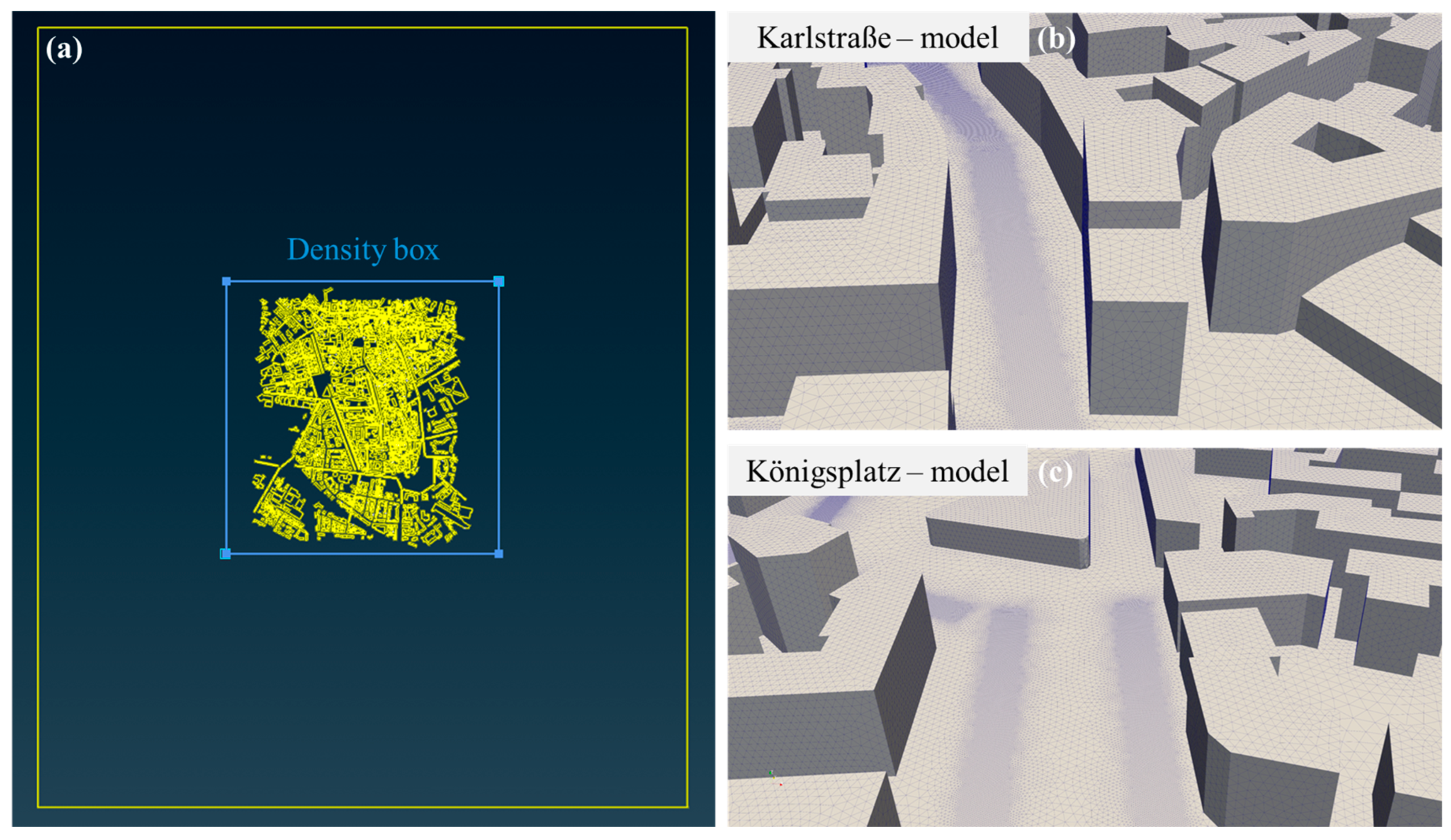
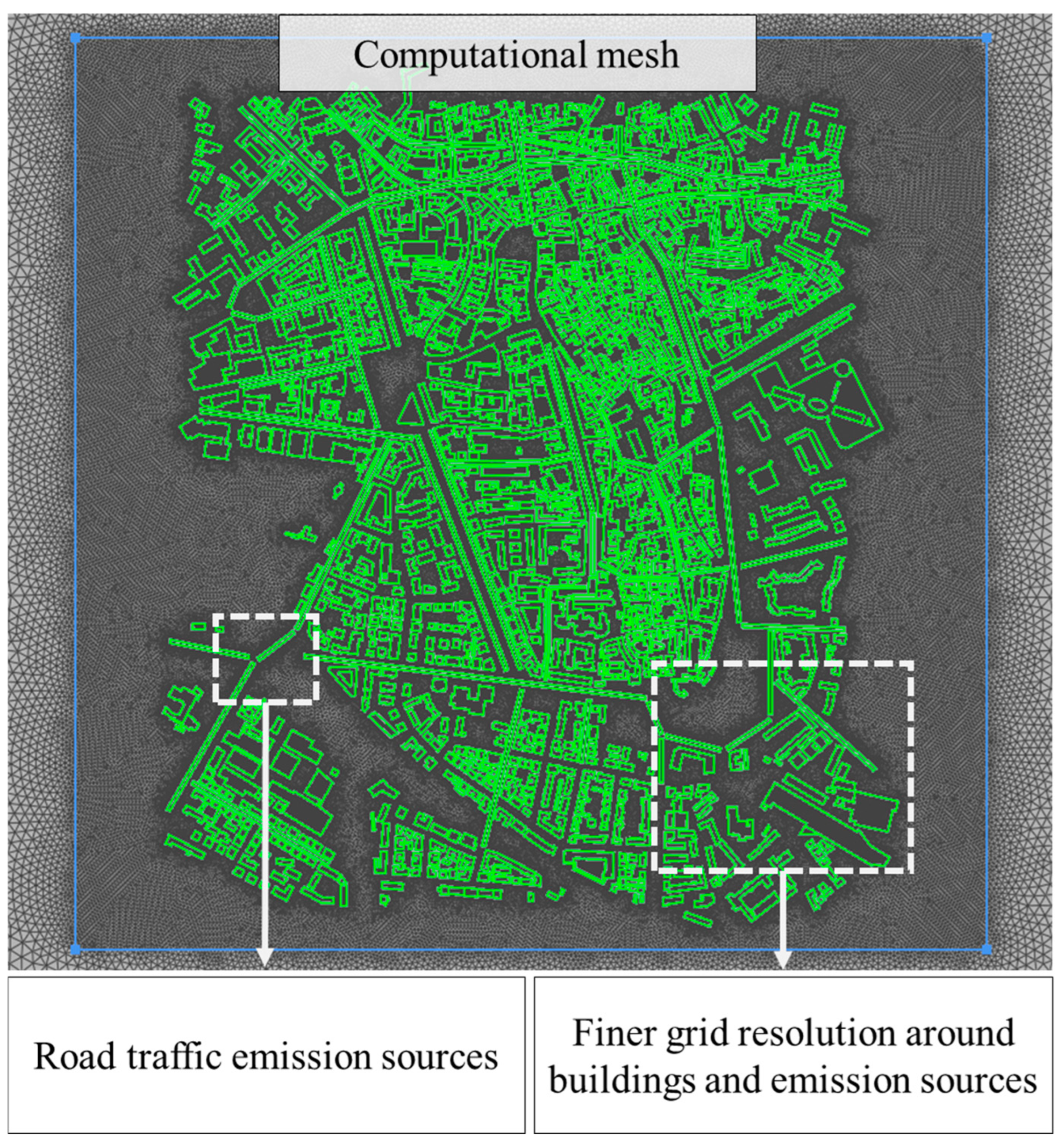
2.1.2. Geometric Model and Computational Grid

In this study, the 3D geometry of the area of interest was created using data from OpenStreetMap (OSM). The raw data were processed to clean and refine building surfaces, a crucial step in preparing a digital grid that integrates the 3D model seamlessly. The refinement process involved reconstructing 3D elements with geometric characteristics identical to the original OSM data using Ansys SpaceClaim 2018, a CAD tool within the Ansys suite designed for geometry creation and processing [21]. Figure 2a displays the developed digital model, highlighting key buildings and emission sources along main arterial roads. The digital domain was built following established guidelines [22]. The computational domain’s height was set to 6Hmax, with an upstream distance of 15Hmax, where Hmax refers to the height of the tallest building in the study area standing at 83.5 m.

A computational grid was created to cover the digital model of the city using the ANSA commercial pre-processor. As shown in Figure 2b, the grid focuses on the area around the KS station, where a surface mesh has been applied to the building and ground surfaces. The rectangular objects depicted at ground level in Figure 2b represent the emission sources, which are strategically placed along both main and smaller roads. Each emission source corresponds to sections of the roads where traffic-related emissions contribute pollutants to the surrounding environment. Figure 2c presents the computational grid developed for the KP station, incorporating both emission sources and detailed building features. The density box shown in Figure 2a serves to define the city’s area and establish a minimum grid size—set to 4 m—ensuring that the regions of interest, such as emission sources and buildings, are refined to the highest level of detail.

The computational mesh created to cover all the domains uses tetrahedral unstructured elements with a growth rate of 1.2. As can be seen in Figure 3, the resolution of the mesh on the buildings and ground is higher compared to the one outside the density box. The grid resolution was set to 1 m for the buildings and ground, while the resolution on the emission sources was set to 0.25 m, ensuring high spatial accuracy in the CFD outputs, particularly in areas near the emission sources and sensor locations. The computational grid consisted of a total of 48 million elements, meeting the high accuracy requirements needed for the convergence of simulations over a 1.6 × 2 km² urban area. The CFD simulations were run on computer nodes equipped with Intel(R) Core™ i9-10980XE@3.00 GHz CPUs. Detailed mesh sensitivity analysis was performed comparing two different grid configurations for this area in a previous study [23]. The comparison between the two grids revealed that this grid required 19 h of computational time, while a finer grid took 37 h to complete, both using the same number of cores and achieving scaled residuals of governing equation parameters below the threshold of 10⁻⁶ as recommended [24]. For this study, the first grid was chosen due to its ability to solve cases twice as fast and its prior use in other published research [21,25].

2.2. Dispersion Model Setup

2.2.1. Numerical Model

The pollutant dispersion modeling in this study was carried out using the open-source CFD software OpenFOAM, with the simpleFoam solver being specifically employed. The simpleFoam solver is a steady-state, pressure-based solver designed for incompressible, turbulent flow simulations. It employs the semi-implicit method for pressure-linked equations (SIMPLE) algorithm to iteratively solve the governing equations while maintaining numerical stability. The governing equations solved are the continuity equation that ensures mass conservation for incompressible flow by enforcing the condition of zero divergence for the mean velocity field (Equation (1)) [26].

$$\nabla \overrightarrow{\cdot U}=0$$

(1)

The simpleFoam solver employs Reynolds-averaged Navier–Stokes (RANS) equations [27,28], which are formulated to capture the mean flow characteristics by averaging the instantaneous equations over time (Equation (2)):

$$\nabla \cdot \left(\overrightarrow{U}\overrightarrow{U}\right)=-{\displaystyle \frac{1}{\rho }}\nabla \mathrm{p}+\nabla \cdot \left[\nu {(\nabla \overrightarrow{U}+(\nabla \overrightarrow{U})}^{{\rm T}}\right)]-\nabla \cdot \overline{\overrightarrow{u\prime }\overrightarrow{u\prime }}$$

(2)

where:

• $\overrightarrow{U}$ represents the mean velocity vector.
• p denotes the mean pressure.
• ρ is the fluid density, which is constant for incompressible flow.
• ν is the kinematic viscosity.

To model the dispersion of pollutants, in Table 1 the passive scalar transport equation (Equation (3)) was incorporated into a modified version of the solver, with the required adaptations compiled into the system. This approach allows for the simulation of passive pollutant dispersion processes [29,30].

In Table 1, Equation (4) represents the turbulent diffusion coefficient (Dt), while Dm corresponds to the molecular diffusion coefficient. For carbon monoxide (CO), the molecular diffusion coefficient at 20 °C is 2.08 × 10⁻⁵ m²/s. Regarding nitrogen oxides (NO_x), which are predominantly composed of NO, part of them undergo atmospheric oxidation to form NO₂ [14]. In this study, NO_x emissions were modeled as a non-reactive pollutant, mostly because the model focuses on near-source dispersion with short transport times, less than the NO oxidation timescales. Overall, the Dm term can be neglected, because in highly turbulent environments, the turbulence diffusion term dominates. The standard k-ε turbulence model was chosen for the RANS simulations due to its well-established effectiveness in urban pollutant dispersion studies [31,32]. This selection was further supported by a review that found that 38% of the reviewed cases favored the standard k-ε model [24].

Table 1. Numerical model information.

Title	Property
Modeling approach	RANS
Turbulent model	k-ε
RANS solver	simpleFoam
Mass transport advection–diffusion equation	${\displaystyle \frac{\partial C}{\partial t}}+{\displaystyle \frac{\partial \left(\overline{u_j}C\right)}{\partial x_j}}-{\displaystyle \frac{\partial }{\partial x_j}}\left(Dt+Dm{\displaystyle \frac{\partial C}{\partial x_j}}\right)=0$ (3) [33]
Turbulence diffusion term (Dt)	$Dt={\displaystyle \frac{vt}{Sct}}$ (4) [34]
Schmidt number (Sct)	0.7 [35]

Table 1. Numerical model information.

Title	Property
Modeling approach	RANS
Turbulent model	k-ε
RANS solver	simpleFoam
Mass transport advection–diffusion equation	${\displaystyle \frac{\partial C}{\partial t}}+{\displaystyle \frac{\partial \left(\overline{u_j}C\right)}{\partial x_j}}-{\displaystyle \frac{\partial }{\partial x_j}}\left(Dt+Dm{\displaystyle \frac{\partial C}{\partial x_j}}\right)=0$ (3) [33]
Turbulence diffusion term (Dt)	$Dt={\displaystyle \frac{vt}{Sct}}$ (4) [34]
Schmidt number (Sct)	0.7 [35]

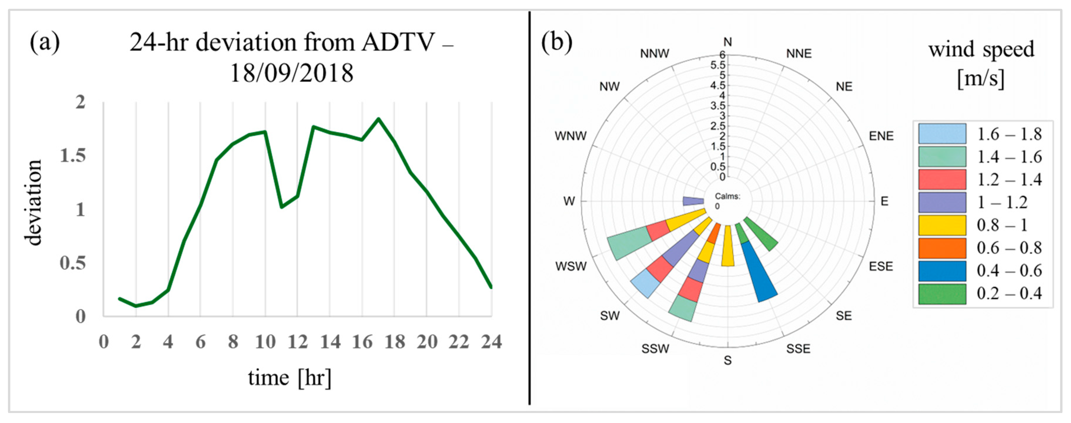
2.2.2. Model Input Data

Emission rates for the traffic-related pollutants (CO and NO_x) were used as inputs for the model. These emissions were calculated based on average daily traffic volume (ADTV) for different road segments during September 2018. The traffic patterns in the case study area represent typical urban conditions. To estimate hourly traffic activity for each road segment, the hourly variation in daily traffic volume was considered, as shown in Figure 4a. This method enabled precise estimation of traffic activity for each road ID, corresponding to the city’s road network. The resulting hourly traffic data allowed for the identification of peak and low traffic periods in the city center. Detailed explanation of the traffic data used can be found in a study that conducted CFD modeling for traffic-related pollutants for Augsburg [16].

Traffic emissions were calculated using COPERT Street software, which estimates pollutant emissions based on traffic activity data. To accurately represent the vehicle fleet in Augsburg, data from the Federal Motor Transport Authority for 2018 were utilized. The fleet composition included passenger cars (73.6%), light commercial vehicles (12.7%), heavy-duty trucks (5.6%), buses (0.6%), and motorcycles (7.5%). An average vehicle speed of 30 km/h was assumed, and the lengths of each road segment were considered in the calculations. The model accounted for emissions from 69 sources, corresponding to multiple road segments and providing a detailed and realistic representation of traffic-related emissions in the study area.

Meteorological data were essential for air quality modeling during the simulation period. Wind speed and direction were measured using a sensor located 1.5 km southeast of the case study area, outside the urban core, ensuring that the data remained unaffected by nearby buildings. As shown in Figure 4b, the prevailing winds during the study period (18 September 2018) predominantly came from the southeast and west, with wind speeds typically ranging from 0.2 to 1.8 m/s.

$$U\left(z\right)={\displaystyle \frac{u^{\mathrm{*}}}{\kappa }}\mathit{ln}\left({\displaystyle \frac{z+z_0}{z}}\right)$$

(5)

To accurately simulate wind flow, an atmospheric boundary layer profile was applied to the model boundaries, ensuring proper wind field development during the simulations. The atmospheric velocity profile, defined by equation (5) [36], was applied at the inlets for each simulation case. In this equation, u* represents the friction velocity, κ is the von Kármán constant (set to 0.41), and z₀ denotes the aerodynamic roughness length specific to urban environments [37]. Simulations to assess the spatial representativeness of the KS and KP air quality stations were conducted using the prevailing wind direction from September 2018, which was predominantly southwestern, as shown in Figure 4b. The period between 13:00 and 14:00 on 18 September 2018 was selected as a test case due to its wind direction of 260 degrees.

The simulations performed for this study represented hourly emission and meteorological conditions. Based on the traffic information for the central area of Augsburg, CO and NO_x emissions were calculated separately for each emission source located in the model. In

Table 2. Total emitted pollutant mass from traffic from all road sources included in the dispersion model during 13:00–14:00. Meteorological information (WS, WD) for the examined time period.

Total CO emitted (kg/h)	10.1
Total NOx emitted (kg/h)	3.1
Wind direction (°)	260
Wind speed (m/s)	1

, the total emitted mass for the examined pollutants from all road sources is shown for the selected time-period. During that time, it was calculated that a total of 10.1 kg/h of CO and 3.1 kg/h of NO_x was emitted by traffic.

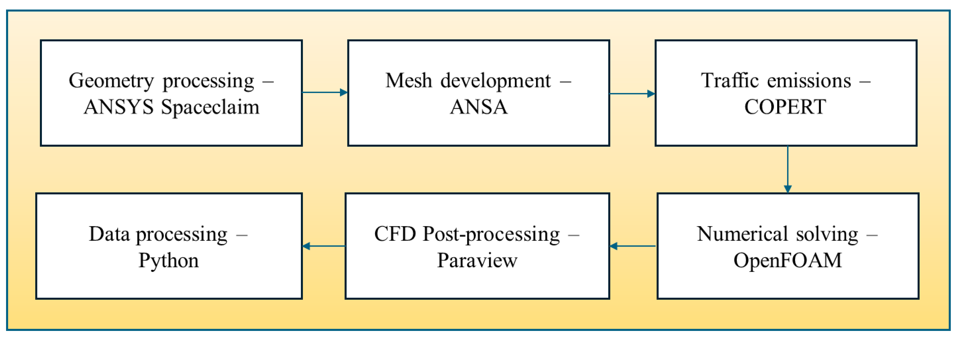
2.2.3. Software Used

During the modeling process, a number of software packages were used to achieve the high-resolution pollution mapping and assessing the air quality station’s coverage for this work. For convenience, Figure 5 depicts the path followed. Firstly, geometry processing was conducted using Ansys SpaceClaim to refine the surfaces of buildings collected from OpenStreetMap and to design the road emission sources. Then, the digital geometry of the city was imported in ANSA for the computational mesh development. The COPERT software was used for the traffic emission calculation for creation of the input data that were to be implemented into the model. For the numerical solving of the cases, OpenFOAM was used and the converged simulations provide the results. To process the CFD-resolved cases, post-processing software, ParaView, was used to visualize and extract variables. Lastly, after extracting all the information needed, the representativity of the air quality stations was assessed by a Python script that accounts for criteria explained in Section 2.3 for the representativeness of the air quality stations.

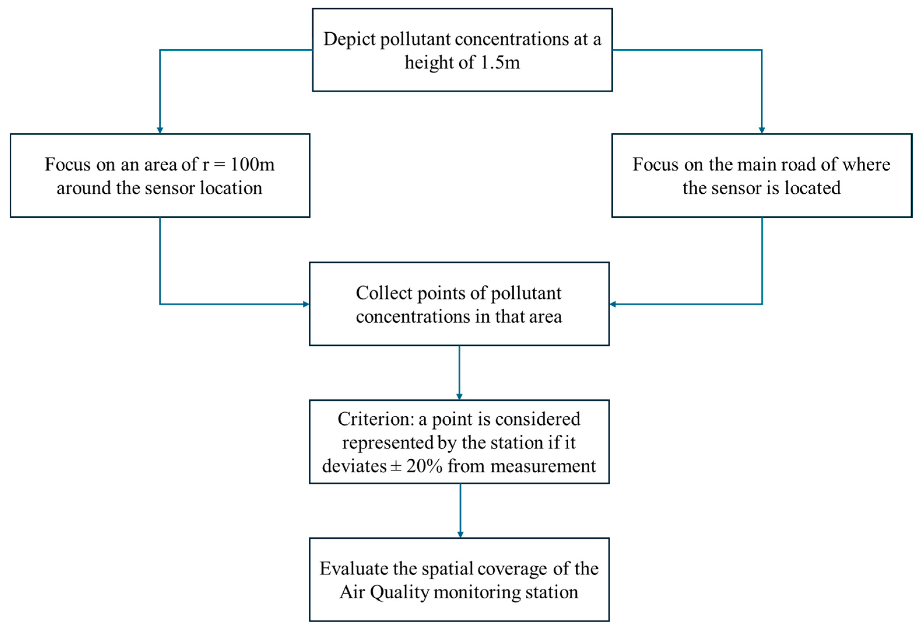
2.3. Methodology Followed for Evaluation of Spatial Representativeness of AQS

To evaluate the representativeness of the air quality (AQ) station measurements, two complementary approaches were used, as illustrated in Figure 6. The first approach involved assessing an area with a 100-m radius around each AQ station. This method captured the spatial variability in pollutant concentrations within the immediate vicinity of the sensor, including both high-traffic roads and adjacent areas with potentially lower traffic activity. By considering this circular area, we aimed to determine whether the AQ station accurately reflected the air quality conditions for the broader environment it represented. The second approach focused specifically on points along the high-traffic roads where the AQ stations were situated. In contrast to the radius-based analysis, this approach isolated locations directly affected by vehicular emissions, highlighting the AQ station’s ability to reflect pollution levels along the most heavily trafficked corridors. Together, these two methods provided valuable insights into the AQ station’s ability to represent both localized and street-specific pollutant concentrations, which are crucial for urban air quality assessments.

To evaluate the model’s performance in these analyses, a representativeness criterion was applied. This criterion considered the AQ station to be representative if simulated pollutant concentrations within the specified area or along the road segments had an absolute deviation of 20% from the observed values [32]. This threshold provided a quantitative measure of agreement, ensuring a robust comparison between simulated and measured concentrations, attributed to traffic activity. The analysis allowed for a detailed examination of the AQ station’s accuracy in capturing pollutant distribution across varying spatial contexts, highlighting its role in reflecting the diverse air quality conditions of the urban microenvironment. This dual-approach evaluation ensured a comprehensive understanding of AQ station performance, shedding light on the extent to which these monitoring points effectively captured pollutant variability in urban settings and aiding in the validation and refinement of air quality models.

3. Results and Discussion

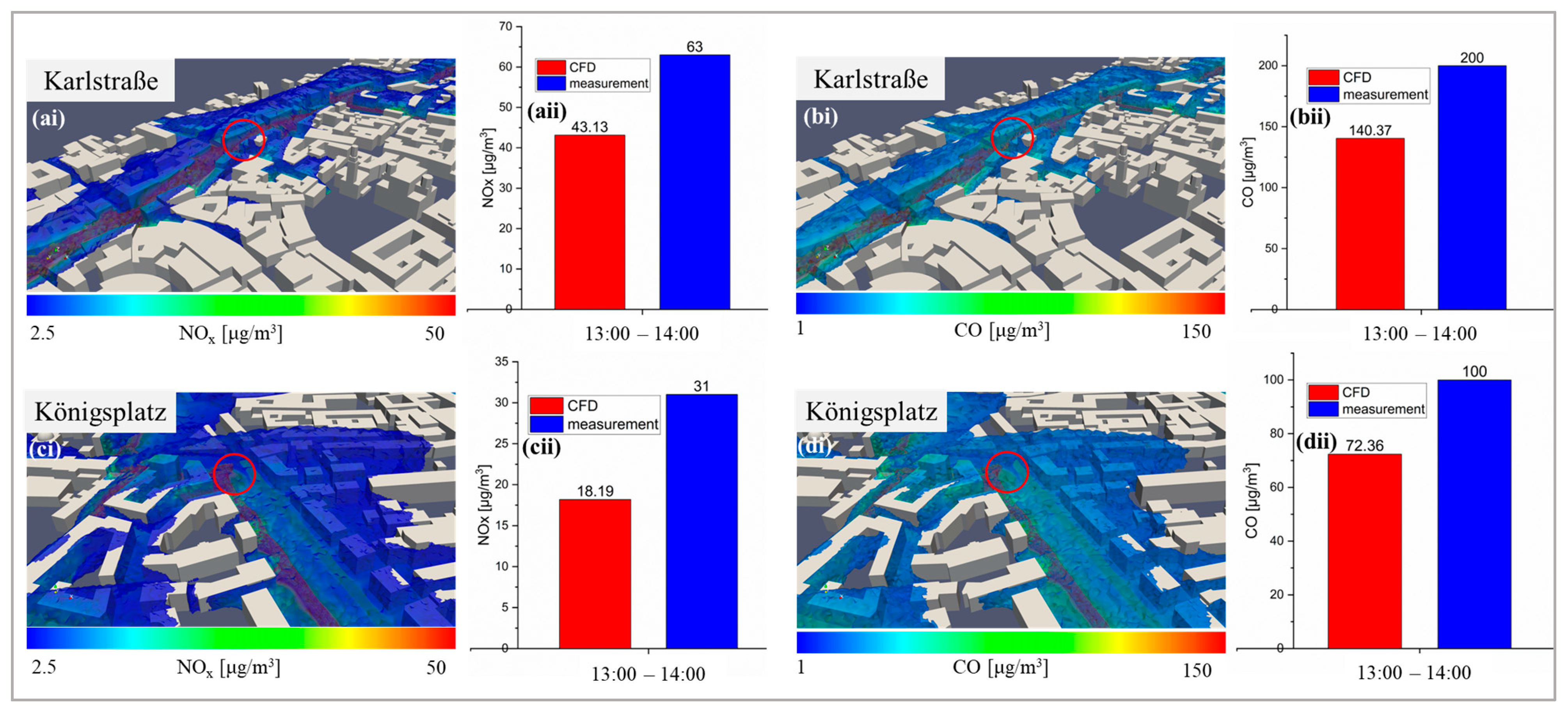
3.1. Dispersion Model Validation

The simulations of traffic-related pollutant dispersion produced concentration values across the entire study area. In order to facilitate a comparison between these simulated concentration values and the actual measurements obtained from monitoring stations, background concentrations recorded at the BP and LFU stations—both of which are located outside the city—were subtracted from the air quality station data taken during the same time intervals. The BP station provided background data for NO_x, and the LFU background station provided measured CO levels. This step was crucial for isolating the specific contribution of street emissions to the pollution levels by removing the effects of background concentrations, which are not influenced by urban activities. These background stations were deliberately placed in locations that are not affected by the urban environment, ensuring that their data accurately reflected baseline atmospheric conditions. By applying this methodology, which aligns with the approach described in [38], a clearer and more precise understanding of the localized impact of urban emissions on air quality was achieved.

Figure 7 shows a detailed comparison between the pollutant concentrations generated by the CFD model and the observed concentrations at the KS and KP stations for the various cases examined. At the KS station, the model demonstrated a reasonable level of performance, with deviations of 29% for carbon monoxide (CO) (Figure 7(aii)) and 31% for nitrogen oxides (NO_x) (Figure 7(bii)). These simulated concentration values were directly associated with the exact position of the station, which was situated at a height of 2.5 m above the ground. For the KP station, the model showed a deviation of 27% for CO (Figure 7(cii)) and 41% for NO_x (Figure 7(dii)). The comparisons were performed at the precise location of the KP station, which was positioned 4 m above the ground. The fact that the modeled values were within the same general range as the measured concentrations, with the percentage deviations primarily attributed to the street-level increment in pollutants, further emphasizes the model’s capability to accurately simulate traffic–related pollution. While some discrepancies were present, they remained within an acceptable range, reinforcing the model’s overall performance. Additionally, the model provided pollutant concentration values with higher decimal precision, which enhanced its reliability and accuracy for conducting fine-scale urban air quality assessment. This level of precision is particularly valuable for understanding localized pollutant concentrations and evaluating the impact of traffic emissions in urban environments. Although the study only covered a 1.6 × 2 km² area, the high spatial resolution the dispersion model provided could be used to recognize high-pollution hotspots affected by local emissions and meteorology. This could be advantageous in the case of dense air quality networks. The results demonstrate that the CFD model can effectively capture the complexities of urban pollutant dispersion, providing useful insights for air quality management and policy development.

To further assess the performance of the dispersion model, we used statistical metrics that can determine whether the simulated results are acceptable based on observations. To achieve that, we used the approach explained in [39]. To calculate the dimensionless concentration C*, in Equation (6), C is the modeled concentration, U_ref is the wind speed for the hour examined, Q is the emission rate of the pollutant, and H is the average building height of the study area, estimated at 15 m. Equations (7)–(9) show FAC2, MG, and VG, metrics that were used here, with O and P corresponding to observed and predicted values.

$${\mathrm{C}}^{\mathrm{*}}={\displaystyle \frac{\mathrm{C}{\mathrm{U}}_{\mathrm{r}\mathrm{e}\mathrm{f}}{\mathrm{H}}^2}{\mathrm{Q}}}$$

(6)

Factor of two (FAC2) counts the fraction of data points where the predictions are within a factor of two of the observations.

$$\mathrm{F}\mathrm{A}\mathrm{C}2={\displaystyle \frac{\mathrm{N}}{\mathrm{n}}}={\displaystyle \frac{1}{\mathrm{n}}}\sum _{\mathrm{i}=1}^{\mathrm{n}}\mathrm{N}\mathrm{i}$$

(7)

Geometric mean bias (MG) is a logarithmic measure of the mean bias.

$$\mathrm{M}\mathrm{G}=\mathrm{e}\mathrm{x}\mathrm{p}(〈\mathrm{l}\mathrm{n}\tilde{\mathrm{O}}〉-〈\mathrm{l}\mathrm{n}\tilde{\mathrm{P}}〉)$$

(8)

Geometric variance (VG) shows the scatter in the data and contains systematic and random errors.

$$\mathrm{V}\mathrm{G}=\mathrm{e}\mathrm{x}\mathrm{p}\left[〈{(\mathrm{l}\mathrm{n}\tilde{\mathrm{O}}-\mathrm{l}\mathrm{n}\tilde{\mathrm{P}})}^2〉\right]$$

(9)

The modeled pollutant concentrations tended to slightly underestimate the measured values, indicating the presence of a systematic bias in the results. This underestimation may be attributed to the inherent limitations of the dispersion model, which only takes into account emissions related to traffic activity. The model does not include other potential sources of urban pollution, such as emissions from households, industrial activities, or cooking operations, which are also significant contributors to the overall pollutant levels in urban environments. Despite this limitation, the model demonstrates good potential to capture the patterns of traffic-related pollution within urban microenvironments, suggesting its suitability for this specific application.

Table 3. Statistical metrics for model performance evaluation based on observations.

	KS CO	KS NOx	KP CO	KP NOx	Ideal	Accepted
FAC2	1.00	1.00	1.00	1.00	1	≥0.5
MG	1.01	1.02	1.01	1.02	1	0.7 ≤ MG ≤ 1.3
VG	1.01	1.01	1.00	1.01	1	≤1.6

shows that after statistical analysis, factors such as FAC2, MG, and VG all lay within the accepted range based on the literature [40]. The analysis was performed with a limited number of data, but it supports the argument of the suitability of the dispersion model. The average deviation of approximately 30% observed across all simulation cases further supports the model’s accepted performance, specifically for traffic-related emissions in urban areas. Studies that have used dispersion modeling to predict pollutant concentrations in urban environments with the use of CFD when compared with observations achieved deviations that could reach 26.9% [41] and 59.7% [31].

This level of accuracy is deemed satisfactory for assessing pollutant dispersion within the study area and provides valuable insights into urban air quality management and planning. While some refinement could improve the model’s ability to account for a broader range of pollution sources, it remains a valuable asset for localized studies of traffic-related air pollution.

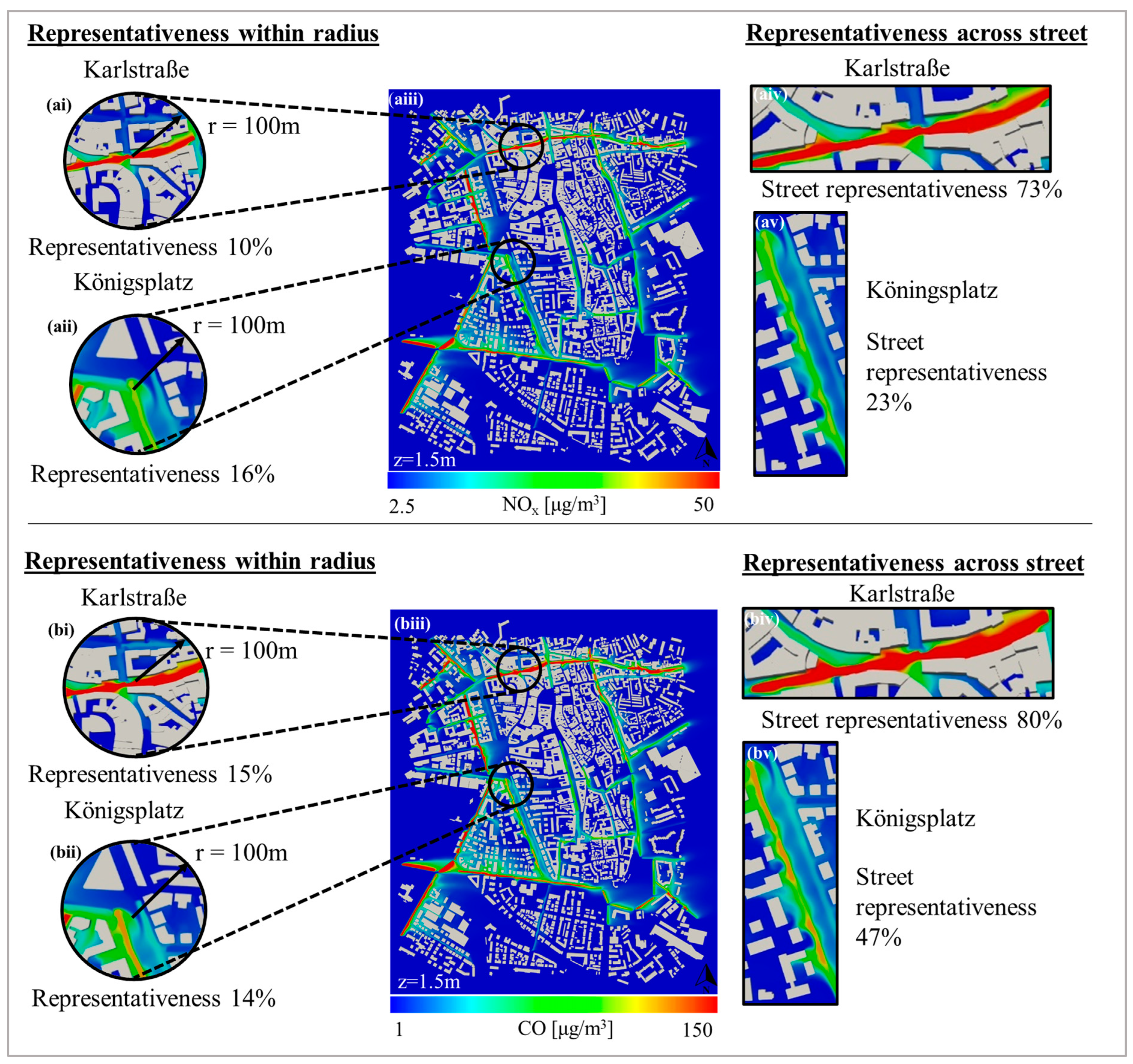
3.2. Spatial Coverage of Air Quality Stations

3.2.1. Representativeness Within a Radius

The CFD model generated high-resolution distribution of pollutant concentrations for CO and NO_x, as depicted in Figure 8. To evaluate the spatial coverage of air quality (AQ) station measurements for these pollutants, we examined a 100-m radius around the sensor locations in the initial representation case. Measurements were taken at a height of 1.5 m, consistent with the exposure height, as shown in Figure 6. For the Karlstraße station, the representativeness values were found to be 15% for CO and 10% for NO_x, as illustrated in Figure 8(ai,bi), respectively. The Königsplatz station exhibited representativeness values of 14% for CO (Figure 8(aii)) and 16% for NO_x (Figure 8(bii)). These results align with similar findings from other studies in the literature. For example, ref. [14] reported a spatial representativeness of 17% for NO₂ concentrations near a traffic monitoring station in Pamplona, where CFD was also utilized for dispersion modeling. Despite this consistency, the relatively low coverage values observed here, 10–16%, may be partially attributed to the specific characteristics of the urban environment around the sensors. One significant factor contributing to this is the high proportion of pedestrian roads in the area.

In particular, for the KS area, the southern side of the 100-m radius consists of a pedestrian zone where no vehicular emissions are present. This lack of vehicular activity results in lower pollutant concentrations in the area, which could reduce the representativeness of the AQ station’s measurements. Similarly, on the northern side of the KS station, the level of road activity is insufficient to generate elevated pollution levels that would typically be detected by the station, because it is characterized by low traffic. A comparable situation was observed for the KP station, where the northern part of the focus area includes a tram station, and no traffic activity data were available for this area. As a result, the model did not generate significant locally influenced concentrations of NO_x or CO in this region. These findings highlight the importance of examining the spatial coverage of sensors using alternative methods, such as focusing on the main arterial road on which the sensor is located. This would provide a more accurate representation of localized air quality and improve the model’s ability to capture the effects of traffic-related pollution.

Another critical consideration is that this study only accounted for traffic emissions as the sole source of pollutants, which may have led to an underestimation of pollutant concentrations. By excluding other urban emission sources—such as those from residential heating, commercial cooking, and industrial activities—the model may not fully capture the range of pollutants affecting air quality. The relatively low representation values observed could therefore reflect this limitation, as the model did not include all relevant emission sources in the area. This highlights the need for future model improvements, specifically the inclusion of additional emission sources, to provide more accurate and comprehensive air quality assessments. These enhancements would also improve the model’s ability to assess pollutant concentrations in diverse urban settings, thereby increasing its applicability and predictive capabilities for various locations.

3.2.2. Street Representativeness

To address the issue of low spatial representativeness within a radius around the air quality (AQ) stations, we explored a second approach that examined the spatial coverage of the monitoring devices along the road on which they were located. In this case, the collected concentration points were taken from an area encompassing the high-traffic roads, with measurements still recorded at a height of 1.5 m, which corresponds to an average exposure height. Given that the monitoring stations are situated in urban traffic hotspots, typically on busy roads, this method was expected to provide a better representation of air quality in the areas directly influenced by vehicular emissions. As shown in Figure 8(aiv,biv), the results indicate that for the Karlstraße station, the street representativeness was significantly higher, with values of 73% for NO_x and 80% for CO. This higher representativeness underscores the ability of the monitoring station to capture pollutant concentrations more accurately along the street, reflecting the impact of traffic emissions in the immediate vicinity. For the Königsplatz station, the model showed a more moderate street representativeness, with values of 23% for NO_x and 47% for CO, as illustrated in Figure 8(av,bv). Although these values were lower than those observed at the Karlstraße station, they still demonstrate the model’s ability to capture traffic-related pollutant concentrations along the street to some extent.

This approach highlights the increased effectiveness of monitoring stations when evaluating pollutant levels along major traffic routes, as they are more likely to reflect the air quality conditions directly influenced by vehicle emissions. By focusing on the road itself rather than a fixed radius, this method provides a more precise understanding of how a station captures the impact of traffic-related pollution.

The dispersion model’s ability to capture the spatial representativeness of air quality (AQ) monitoring stations significantly improved when the analysis was extended to encompass the area across the main road on which the station is located compared to using a fixed radius around the sensor. This improvement was due to the fact that higher traffic-related concentrations are more effectively modeled in areas with greater vehicular activity, which are typically found along major roads. By focusing on these high-traffic areas, the model can more accurately represent pollutant levels directly influenced by traffic emissions. The results obtained from this approach fell within the acceptable range defined by the 20% criterion for observation from the station, which is positioned at a strategically chosen location along the street to best capture the pollution levels associated with traffic. This indicates that the model’s predictions align closely with the station’s measurements in areas directly impacted by traffic. This highlights the importance of considering the specific context of a monitoring station’s location when evaluating its ability to represent urban air quality.

4. Conclusions

This study successfully developed and applied a CFD model to assess air quality, focusing primarily on traffic-related emissions. The model was validated by comparing its outputs with data from two official air quality monitoring stations located within a 1.6 × 2 km² area. The average deviation between the modeled and measured concentrations was 29% for NO_x and 31% for CO at the Karlstraße (KS) station, while at the Königsplatz (KP) station, the deviations were 41% for NOx and 27% for CO. Despite these differences, all simulated values remained within the range of observed measurements, indicating that the model provided reasonably accurate results. To assess the representativeness of the air quality stations, a maximum absolute deviation of 20% from the measured values was used as the criterion. The analysis was conducted in two ways: within a 100-m radius around each station and along the road where the monitoring devices were located. This approach allowed for a focused evaluation of local pollution levels, providing insights into how well the stations represent air quality in both their immediate vicinity and in high-traffic areas.

The results showed that the Karlstraße station had a representativeness of 10% and 16% for NO_x and CO, respectively, when considering a 100-m radius. Similarly, the Königsplatz station exhibited representativeness values of 16% for NO_x and 14% for CO. The relatively low coverage observed in this study can be partly attributed to the urban landscape surrounding the sensors, particularly the presence of pedestrian areas, which reduce traffic-related emissions and lower pollutant concentrations. For example, the southern side of the 100-m radius around the Karlstraße station is pedestrianized, while the northern side has minimal road activity, making it less representative of the station’s location at a traffic hotspot. Likewise, the northern area near the Königsplatz station includes a tram station for which no traffic data were available, further decreasing the likelihood of elevated NO_x and CO concentrations in that area.

When assessing the spatial coverage of the monitoring stations across the street from their locations, the methodology used in this study showed higher representativity. For the Karlstraße station, the coverage reached 73% for NO_x and 80% for CO, while for the Königsplatz station, the street representativeness was 23% for NO_x and 47% for CO. Areas with higher traffic-related concentrations tended to be modeled more accurately, which aligns with the 20% deviation criterion relative to the station’s observations. These observations were taken from strategically placed locations intended to effectively capture pollution levels. The analysis underscores that air quality stations are more representative of pollution generated in high-activity areas around the street of their deployment, rather than in the surrounding lower-activity zones.

By evaluating the spatial representativeness of the air quality stations within a limited area close to the sensors, the study effectively determined the appropriateness of station placements and whether their measurements truly reflected the surrounding pollution conditions. This analysis helps ensure that the sensor locations accurately capture the air quality in the area they monitor. The findings highlight the influence of local emission sources, meteorological conditions, and urban structures on pollutant dispersion, reinforcing the importance of carefully selecting monitoring sites. Additionally, the study underscores the limitations of fixed monitoring stations in capturing fine-scale air pollution variations, suggesting that complementary approaches such as mobile sensors or computational modeling could enhance spatial coverage. Future research could focus on integrating low-cost sensor networks and advanced modeling techniques to refine pollution exposure assessments and improve urban air quality management strategies.

References

1. Ju, K.; Lu, L.; Wang, W.; Chen, T.; Yang, C.; Zhang, E.; Xu, Z.; Li, S.; Song, J.; Pan, J.; et al. Causal Effects of Air Pollution on Mental Health among Adults—An Exploration of Susceptible Populations and Role of Physical Activity Based on a Longitudinal Nationwide Cohort in China. Environ. Res. 2022, 217, 114761. [Google Scholar] [CrossRef] [PubMed]
2. Piracha, A.; Chaudhary, M.T. Urban Air Pollution, Urban Heat Island and Human Health: A Review of the Literature. Sustainability 2022, 14, 9234. [Google Scholar] [CrossRef]
3. Schwela, D.H.; Haq, G. Strengths and Weaknesses of the WHO Urban Air Pollutant Database. Aerosol Air Qual. Res. 2020, 20, 1026–1037. [Google Scholar] [CrossRef]
4. Zhang, J.J.; Wei, Y.; Fang, Z. Ozone Pollution: A Major Health Hazard Worldwide. Front. Immunol. 2019, 10, 2518. [Google Scholar] [CrossRef]
5. Reşitoğlu, I.A.; Altinişik, K.; Keskin, A. The Pollutant Emissions from Diesel-Engine Vehicles and Exhaust Aftertreatment Systems. Clean. Technol. Environ. Policy 2015, 17, 15–27. [Google Scholar] [CrossRef]
6. Grewe, V.; Dahlmann, K.; Matthes, S.; Steinbrecht, W. Attributing Ozone to NOx Emissions: Implications for Climate Mitigation Measures. Atmos. Environ. 2012, 59, 102–107. [Google Scholar] [CrossRef]
7. Angatha, R.K.; Mehar, A. Impact of Traffic on Carbon Monoxide Concentrations Near Urban Road Mid-Blocks. J. Inst. Eng. (India) Ser. A 2020, 101, 713–722. [Google Scholar] [CrossRef]
8. Chen, R.; Pan, G.; Zhang, Y.; Xu, Q.; Zeng, G.; Xu, X.; Chen, B.; Kan, H. Ambient Carbon Monoxide and Daily Mortality in Three Chinese Cities: The China Air Pollution and Health Effects Study (CAPES). Sci. Total Environ. 2011, 409, 4923–4928. [Google Scholar] [CrossRef]
9. Paul, T.; Riedel, T.; Matthias, B. Spatial Interpolation of Air Quality Data with 616 Multidimensional Gaussian Processes. INFORMATIK 2021; 2. Workshop Künstliche Intelligenz 618 in der Umweltinformatik (KIUI-2021), Berlin, 27 September–1 October 2021; Gesellschaft für Informatik: Bonn, Germany, 2021; pp. 269–286. PISSN: 1617-5468; ISBN 978-3-88579-708-1. [Google Scholar] [CrossRef]
10. Nguyen, N.H.; Nguyen, H.X.; Le, T.T.B.; Vu, C.D. Evaluating Low-Cost Commercially Available Sensors for Air Quality Monitoring and Application of Sensor Calibration Methods for Improving Accuracy. Open J. Air Pollut. 2021, 10, 1–17. [Google Scholar] [CrossRef]
11. Munir, S.; Mayfield, M.; Coca, D.; Jubb, S.A.; Osammor, O. Analysing the Performance of Low-Cost Air Quality Sensors, Their Drivers, Relative Benefits and Calibration in Cities—A Case Study in Sheffield. Environ. Monit. Assess. 2019, 191, 94. [Google Scholar] [CrossRef]
12. Office of the European Union L-, P.; Luxembourg, L. Directive (EU) 2024/2881 of the European Parliament and of the Council of 23 October 2024 on Ambient Air Quality and Cleaner Air for Europe (Recast). Off. J. Eur. Union 2024, L 2881, 1–50. [Google Scholar]
13. Santiago, J.L.; Borge, R.; Sanchez, B.; Quaassdorff, C.; de la Paz, D.; Martilli, A.; Rivas, E.; Martín, F. Estimates of Pedestrian Exposure to Atmospheric Pollution Using High-Resolution Modelling in a Real Traffic Hot-Spot. Sci. Total Environ. 2021, 755, 142475. [Google Scholar] [CrossRef] [PubMed]
14. Rivas, E.; Santiago, J.L.; Lechón, Y.; Martín, F.; Ariño, A.; Pons, J.J.; Santamaría, J.M. CFD Modelling of Air Quality in Pamplona City (Spain): Assessment, Stations Spatial Representativeness and Health Impacts Valuation. Sci. Total Environ. 2019, 649, 1362–1380. [Google Scholar] [CrossRef] [PubMed]
15. Piersanti, A.; Vitali, L.; Righini, G.; Cremona, G.; Ciancarella, L. Spatial Representativeness of Air Quality Monitoring Stations: A Grid Model Based Approach. Atmos. Pollut. Res. 2015, 6, 953–960. [Google Scholar] [CrossRef]
16. Ioannidis, G.; Li, C.; Tremper, P.; Riedel, T.; Ntziachristos, L. Application of CFD Modelling for Pollutant Dispersion at an Urban Traffic Hotspot. Atmosphere 2024, 15, 113. [Google Scholar] [CrossRef]
17. Boikos, C.; Ioannidis, G.; Rapkos, N.; Tsegas, G.; Katsis, P.; Ntziachristos, L. Estimating Daily Road Traffic Pollution in Hong Kong Using CFD Modelling: Validation and Application. Build. Environ. 2025, 267, 112168. [Google Scholar] [CrossRef]
18. Idrissi, M.S.; Lakhal, F.A.; Ben Salah, N.; Chrigui, M. CFD Modeling of Air Pollution Dispersion in Complex Urban Area. In Lecture Notes in Mechanical Engineering; Springer: Heidelberg, Germany, 2018; pp. 1191–1203. [Google Scholar]
19. Lauriks, T.; Longo, R.; Baetens, D.; Derudi, M.; Parente, A.; Bellemans, A.; van Beeck, J.; Denys, S. Application of Improved CFD Modeling for Prediction and Mitigation of Traffic-Related Air Pollution Hotspots in a Realistic Urban Street. Atmos. Environ. 2021, 246, 118127. [Google Scholar] [CrossRef]
20. Toscano, D.; Marro, M.; Mele, B.; Murena, F.; Salizzoni, P. Assessment of the Impact of Gaseous Ship Emissions in Ports Using Physical and Numerical Models: The Case of Naples. Build. Environ. 2021, 196, 107812. [Google Scholar] [CrossRef]
21. Antoniou, A.; Ioannidis, G.; Ntziachristos, L. Realistic Simulation of Air Pollution in an Urban Area to Promote Environmental Policies. Environ. Model. Softw. 2024, 172, 105918. [Google Scholar] [CrossRef]
22. Blocken, B. Computational Fluid Dynamics for Urban Physics: Importance, Scales, Possibilities, Limitations and Ten Tips and Tricks towards Accurate and Reliable Simulations. Build. Environ. 2015, 91, 219–245. [Google Scholar] [CrossRef]
23. Ioannidis, G.; Tremper, P.; Li, C.; Riedel, T.; Rapkos, N.; Boikos, C.; Ntziachristos, L. Integrating Cost-Effective Measurements and CFD Modeling for Accurate Air Quality Assessment. Atmosphere 2024, 15, 1056. [Google Scholar] [CrossRef]
24. Pantusheva, M.; Mitkov, R.; Hristov, P.O.; Petrova-Antonova, D. Air Pollution Dispersion Modelling in Urban Environment Using CFD: A Systematic Review. Atmosphere 2022, 13, 1640. [Google Scholar] [CrossRef]
25. Gkirmpas, P.; Tsegas, G.; Ioannidis, G.; Vlachokostas, C.; Moussiopoulos, N. Identification of an Unknown Stationary Emission Source in Urban Geometry Using Bayesian Inference. Atmosphere 2024, 15, 871. [Google Scholar] [CrossRef]
26. Olivardia, F.G.G.; Zhang, Q.; Matsuo, T.; Shimadera, H.; Kondo, A. Analysis of Pollutant Dispersion in a Realistic Urban Street Canyon Using Coupled CFD and Chemical Reaction Modeling. Atmosphere 2019, 10, 479. [Google Scholar] [CrossRef]
27. Peralta, C.; Nugusse, H.; Kokilavani, S.P.; Schmidt, J.; Stoevesandt, B. Validation of the SimpleFoam (RANS) Solver for the Atmospheric Boundary Layer in Complex Terrain. ITM Web Conf. 2014, 2, 01002. [Google Scholar] [CrossRef]
28. Rapkos, N.; Boikos, C.; Ioannidis, G.; Ntziachristos, L. Direct Deposition of Air Pollutants in the Wake of Container Vessels: The Missing Term in the Environmental Impact of Shipping. Atmos. Pollut. Res. 2024, 15, 102013. [Google Scholar] [CrossRef]
29. Elfverson, D.; Lejon, C. Use and Scalability of Openfoam for Wind Fields and Pollution Dispersion with Building-and Ground-Resolving Topography. Atmosphere 2021, 12, 1124. [Google Scholar] [CrossRef]
30. Miao, Y.; Liu, S.; Zheng, Y.; Wang, S.; Li, Y. Numerical Study of Traffic Pollutant Dispersion within Different Street Canyon Configurations. Adv. Meteorol. 2014, 2014, 458671. [Google Scholar] [CrossRef]
31. Amorim, J.H.; Rodrigues, V.; Tavares, R.; Valente, J.; Borrego, C. CFD Modelling of the Aerodynamic Effect of Trees on Urban Air Pollution Dispersion. Sci. Total Environ. 2013, 461–462, 541–551. [Google Scholar] [CrossRef]
32. Santiago, J.L.; Martín, F.; Martilli, A. A Computational Fluid Dynamic Modelling Approach to Assess the Representativeness of Urban Monitoring Stations. Sci. Total Environ. 2013, 454–455, 61–72. [Google Scholar] [CrossRef]
33. Dehghan, M. Numerical Solution of the Three-Dimensional Advection-Diffusion Equation. Appl. Math. Comput. 2004, 150, 5–19. [Google Scholar] [CrossRef]
34. Vanderwel, C.; Tavoularis, S. Measurements of Turbulent Diffusion in Uniformly Sheared Flow. J. Fluid. Mech. 2014, 754, 488–514. [Google Scholar] [CrossRef]
35. Tominaga, Y.; Stathopoulos, T. Turbulent Schmidt Numbers for CFD Analysis with Various Types of Flowfield. Atmos. Environ. 2007, 41, 8091–8099. [Google Scholar] [CrossRef]
36. Yang, Y.; Gu, M.; Chen, S.; Jin, X. New Inflow Boundary Conditions for Modelling the Neutral Equilibrium Atmospheric Boundary Layer in Computational Wind Engineering. J. Wind. Eng. Ind. Aerodyn. 2009, 97, 88–95. [Google Scholar] [CrossRef]
37. Irwan Ramli, N.; Idris Ali, M.; Saad, H. Estimation of the Roughness Length (zo) in Malaysia Using Satellite Image. In Proceedings of the Seventh Asia-Pacific Conference on Wind Engineering, Taipei, Taiwan, 8–12 November 2009. [Google Scholar]
38. Jeanjean, A.; Buccolieri, R.; Eddy, J.; Monks, P.; Leigh, R. Air Quality Affected by Trees in Real Street Canyons: The Case of Marylebone Neighbourhood in Central London. Urban For. Urban Green. 2017, 22, 41–53. [Google Scholar] [CrossRef]
39. Di Sabatino, S.; Buccolieri, R.; Olesen, H.R.; Ketzel, M.; Berkowicz, R.; Franke, J.; Schatzmann, M.; Schlünzen, K.H.; Leitl, B.; Britter, R.; et al. COST 732 in Practice: The MUST Model Evaluation Exercise. Int. J. Environ. Pollut. 2011, 44, 403–418. [Google Scholar] [CrossRef]
40. Di Sabatino, S.; Buccolieri, R.; Pulvirenti, B.; Britter, R. Simulations of Pollutant Dispersion within Idealised Urban-Type Geometries with CFD and Integral Models. Atmos. Environ. 2007, 41, 8316–8329. [Google Scholar] [CrossRef]
41. Boikos, C.; Siamidis, P.; Oppo, S.; Armengaud, A.; Tsegas, G.; Mellqvist, J.; Conde, V.; Ntziachristos, L. Validating CFD Modelling of Ship Plume Dispersion in an Urban Environment with Pollutant Concentration Measurements. Atmos. Environ. 2024, 319, 120261. [Google Scholar] [CrossRef]
42. Ioannidis, G.; Riedel, T.; Li, C.; Tremper, P.; Ntziachristos, L. A Numerical CFD Model to Quantify Traffic-Related Pollutant Concentrations in Urban Scale. In Proceedings of the Transport & Air Pollution (TAP) Conference, Gothenburg, Sweden, 25–28 September 2023. [Google Scholar]
Figure 1. Study area and positions of air quality monitoring stations (a). Focus on areas surrounding Karlstraße AQS (b) and Königsplatz AQS (c). Images taken from © Google Earth.
Atmosphere 16 00326 g001
Figure 2. Digital model and computational domain characteristics (a). Focus on the computational mesh developed for Karlstraße area (b) and Königsplatz area (c).
Atmosphere 16 00326 g002
Figure 3. Computational mesh developed for this work. Emission sources placed across main arterial roads and illustration of enhanced grid resolution in areas of interest.
Atmosphere 16 00326 g003
Figure 4. Deviations from average daily traffic volume (ADTV) during the 24-hour period examined for the road IDs contained in the model (a). Wind speed (WS) and wind direction (WD) for the examined period observed by the meteorological station (b).
Atmosphere 16 00326 g004
Figure 5. Diagram of software used in this study.
Atmosphere 16 00326 g005
Figure 6. Methodology followed to identify the spatial coverage of the air quality monitoring stations using the CFD dispersion model introduced in this work.
Atmosphere 16 00326 g006
Figure 7. Traffic-–related pollutant concentrations generated by the CFD model for Karlstraße (ai,bi) and Königsplatz (ci,di) for CO and NOx. Comparisons between the street increment of measurements and CFD for CO and NOx for the cases of Karlstraße (KS) (aii,bii) and Königsplatz (KP) (cii,dii).
Atmosphere 16 00326 g007
Figure 8. Assessment of representativeness of KS and KP monitoring stations for CO and NOx. Two different approaches were followed for evaluating the spatial coverage of the sensors: (1) within a radius of 100 m from the sensor position for NOx (ai,aii) and CO (bi,bii) and (2) within the street that the sensor is located in for NOx (aiv,av) and CO (biv,bv). The pollutant distribution for the whole domain is shown in (aiii) for NOx and (biii) for CO.
Atmosphere 16 00326 g008