Article

Assessing the Spatiotemporal Dynamics and Health Impacts of Surface Ozone Pollution in Beijing, China

by
Fangxu Yin
1,2,
Jiewen You
1,3,* and
Lu Gao
1,3
1
School of Geographical Sciences, Fujian Normal University, Fuzhou 350007, China
2
School of Geography, Earth and Environmental Science, University of Birmingham, Edgbaston, Birmingham B15 2TT, UK
3
Fujian Provincial Engineering Research Center for Monitoring and Assessing Terrestrial Disasters, Fujian Normal University, Fuzhou 350007, China
*
Author to whom correspondence should be addressed.
Atmosphere 2025, 16(4), 397; https://doi.org/10.3390/atmos16040397
Submission received: 11 March 2025 / Revised: 27 March 2025 / Accepted: 28 March 2025 / Published: 29 March 2025
(This article belongs to the Special Issue Atmospheric Pollution in Highly Polluted Areas)

Abstract

:
Surface ozone has emerged as a concerning pollutant in Beijing, China. This study assessed ozone pollution and its health impacts in Beijing using ground (35 stations) and satellite data (2014–2023). Temporal trends were analyzed across various temporal scales, while spatial variability was evaluated using integrated ground and satellite-derived continuous data. Health impacts were quantified via a log-linear concentration–response model. Results show that for ozone concentrations during the post-pandemic period (2019–2023, covering the onset of COVID-19 in 2019 and the period following), daytime concentrations decreased by 6.8 μg/m3, but nighttime concentrations increased by 5.4 μg/m3. Spatially, ozone concentrations were higher in urban areas than in suburban areas in summer, but the reverse occurred in other seasons. Satellite data revealed broader Grade II (160 μg/m3) exceedance variability (3.0–20.3%) compared to station estimates (15.3–18.7%). Health impact assessments indicated that achieving the Grade I standard (100 μg/m3) could prevent approximately 576 (95% CI: 317–827) all-cause deaths and 294 (95% CI: 111–467) cardiovascular deaths per year, which is 3.5 times more than the reductions from meeting the Grade II standard (160 μg/m3). These findings underscore the need for adaptive ozone controls and tiered mitigation strategies to reduce health risks in Beijing.

1. Introduction

Rapid urbanization and industrialization have led to a significant increase in the atmospheric emissions of various pollutants. According to the Global Burden of Disease Study, air pollution was among the leading risk factors contributing to the global disease burden in 2021 [1]. Given its severity, many preventive and control measures have been taken around the world to address the problem, including in China, a country severely affected by air pollution [2]. The Chinese government has initiated an intensive set of national actions since 2013, including the Action Plan for Air Pollution Prevention and Control from 2013 to 2017, and a three-year action plan to win the “Blue-Sky Defence Battle” from 2018 to 2020. The current focus of pollution control measures has predominantly centered on reducing particulate matter pollution such as PM2.5, yielding significant progress [3]. However, success in reducing PM2.5 pollution has been accompanied by an exacerbation of ozone pollution in recent years [4]. In the warmer months (June to August), ground-level ozone has emerged as the primary air pollutant in China [5,6], raising concerns about its health effects, such as increased cardiovascular diseases and premature mortality [7,8,9].
Ground-level ozone is considered a secondary pollutant, forming due to photochemical reactions involving carbon monoxide, nitrogen oxides, and volatile organic compounds under the influence of solar radiation [10]. Its participation in atmospheric chemical reactions contributes to the creation of photochemical smog, which is known to have detrimental health effects. With its strong irritant properties, elevated ground-level ozone concentrations can adversely affect various human organs, including the respiratory and immune systems, skin, and other tissues. This poses significant health risks, threatening forests and biodiversity [11,12]. Given the large population and the prevalence of harmful levels of ozone exposure, understanding the characteristics and health impacts of ozone exposure is crucial for safeguarding public health.
Ground-based monitoring data can offer an accurate localized description of ozone pollution characteristics. However, due to the high cost, it is impossible to deploy air pollution monitoring stations everywhere, making this traditional fixed-point monitoring sparse in spatial coverage [13,14]. Moreover, an uneven distribution of stations, which are either concentrated or far from the pollution hotspots, can also make it difficult to reveal the spatial and temporal patterns and dynamic evolution of ozone exposure accurately and deeply [15]. Spatial interpolations, such as inverse distance weighting, are widely used in environmental studies, including ozone pollution studies [16,17,18]. These methods offer estimates for areas with sparse data and enable the creation of continuous maps and, therefore, have been adopted in many studies. Apart from spatial interpolation, satellite-based methods [19] and air quality models can also estimate ambient ozone concentration in areas with limited ground-based stations [20].
Ambient ozone concentration is not the same as exposure. To convert ambient ozone concentration into ozone exposure, a health impact function is required. This function defines the relationship between changes in ozone concentration and their effects on public health outcomes, such as premature mortality due to cardiovascular diseases, respiratory illnesses (e.g., chronic obstructive pulmonary disease, asthma), and neurological conditions (e.g., stroke) [21,22,23,24,25]. The assessment relies on various epidemiological cohort studies to establish a concentration–response relationship between ozone pollution and health outcomes, which can allow for a quantitative assessment of health risks [23,26,27,28].
Global studies have examined the spatiotemporal patterns and health impacts of ozone pollution, including research in the US [29], Netherlands [30], and India [31], as well as national analyses in China [32]. And some studies focused on Beijing [33,34]. Beijing, a densely populated megacity (over 20,000 persons per km² in urban districts [35]) with severe ozone pollution challenges, highlights the critical necessity to comprehensively understand its spatiotemporal pollution patterns and quantify the health benefits of ozone mitigation measures. Previous studies have often focused on the variation in and influencing factors of ozone pollution in Beijing [36,37,38,39,40]. However, systematic evaluations of ozone compliance with national standards and the health benefits of control measures, including comparisons between pre-pandemic (2014–2018) and post-pandemic (2019–2023) periods, remain insufficiently explored. This is particularly critical in the context of policy-making and ozone regulation in Beijing and similar megacities worldwide.
In this study, we investigated the compliance of ozone pollution and its health impacts under the tiered air quality standards specified in the National Ambient Air Quality Standard in China. The Grade I standard requires ozone concentrations under 100 μg/m3 for ecologically sensitive areas like natural reserves, and the Grade II standard sets 160 μg/m3 as a threshold in urban and industrial zones. These standards guide pollution control policies and reflect a balance between environmental protection and socioeconomic feasibility. We first analyzed temporal patterns across hourly, daily, seasonal, and pre-/post-pandemic periods, then quantified spatial heterogeneity in ozone distribution and exceedance rates, identifying discrepancies between station-based monitoring and satellite-derived continuous data. The study period was split into pre-pandemic (2014–2018) and post-pandemic (2019–2023) to assess long-term trends and the influence of the COVID-19 pandemic, which emerged in late 2019 and led to significant emission changes from 2020 onward due to lockdowns. Finally, to estimate the potential health benefits of meeting stricter air quality standards, we applied the health impact function, which is the mathematical model quantifying the relationship between ozone concentration changes and specific health outcomes, including mortality. These functions, derived from epidemiological data, were used with a log-linear model to calculate the avoidable deaths over the 10-year period under the assumption of Grade I compliances and Grade II compliances. The findings of this study can provide valuable implications for ozone pollution control, particularly in the context of highly populated regions.

2. Materials and Methods
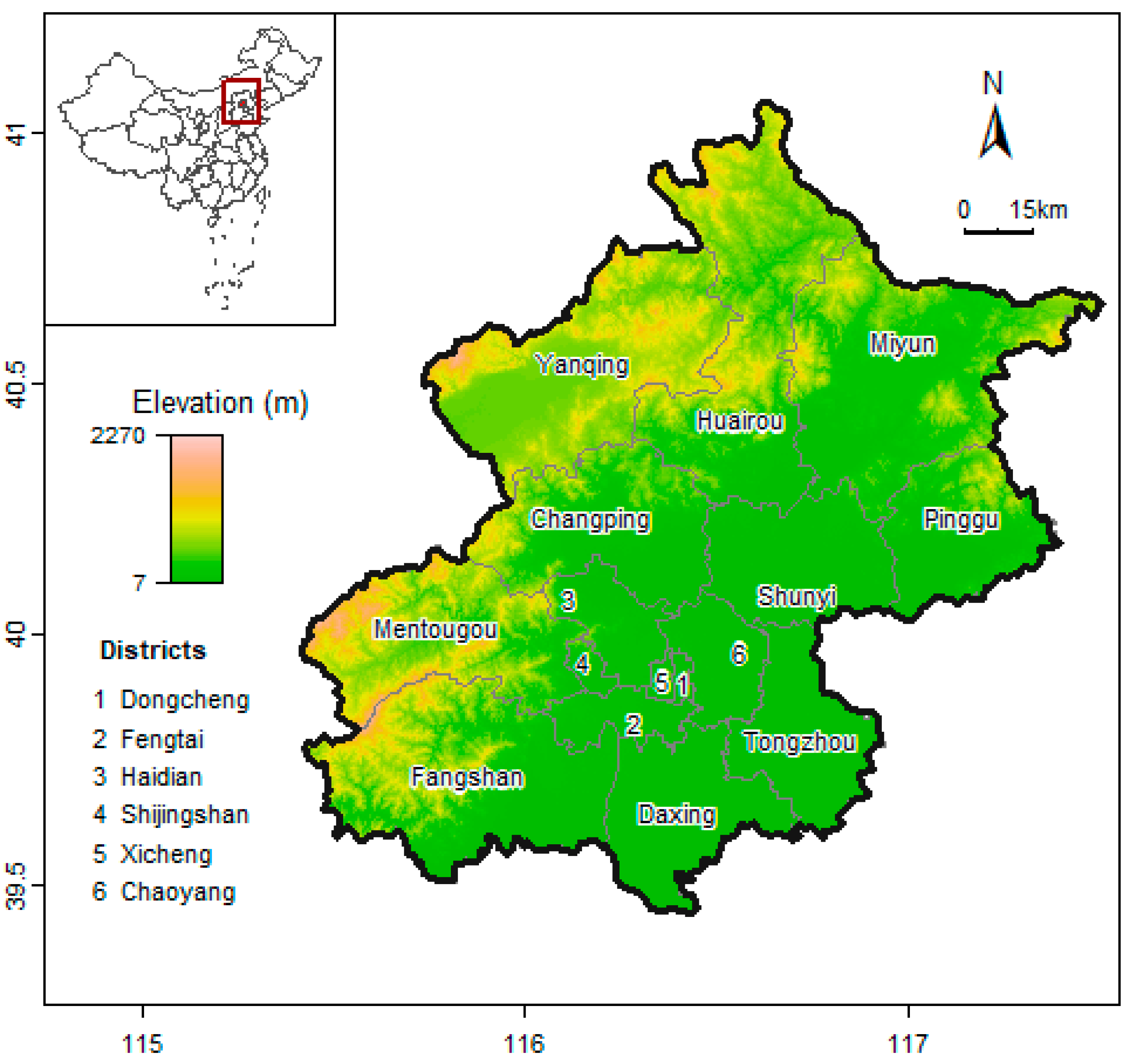
2.1. Study Area

Figure 1 shows the geographic location of Beijing and its 16 administrative districts. As the capital city of China, Beijing has a total area of approximately 16,410 km². In 2014, its population was recorded at 21.52 million, increasing to 21.86 million by 2023. Its topography consists mainly of the North China plains with Yan Mountain in the northwest and northern outskirts. Beijing experiences a continental monsoon climate characterized by hot, humid summers and cold, dry winters. The region is influenced by the East Asian monsoon system, with different high-pressure systems prevailing in winter and summer. These meteorological conditions greatly affect the transport, dispersion, and formation of ozone and other air pollutants.
The rapid urbanization and industrial development of the city have resulted in numerous anthropogenic activities contributing to ozone pollution. The city’s population, industrial sectors, transportation systems, and energy consumption are major sources of ozone precursors such as nitrogen oxides, volatile organic compounds, and carbon monoxide. Emissions from fossil fuel combustion, industrial processes, vehicle exhaust, and residential activities significantly contribute to the high levels of ozone pollution observed in Beijing.

2.2. Data Collection and Processing

In this study, five crucial datasets were used to conduct our analysis: ground-level ozone observations, satellite-based ozone concentration, gridded population data, baseline mortality data, and concentration–response relationship data. We used a daily maximum 8 h average (MDA8) metric for daily ozone estimation. Our study period spans from 1 January 2014 to 31 December 2023, and we collected data specifically during this time period. We began the analysis in 2014, as the available ozone data for Beijing started in December 2013.

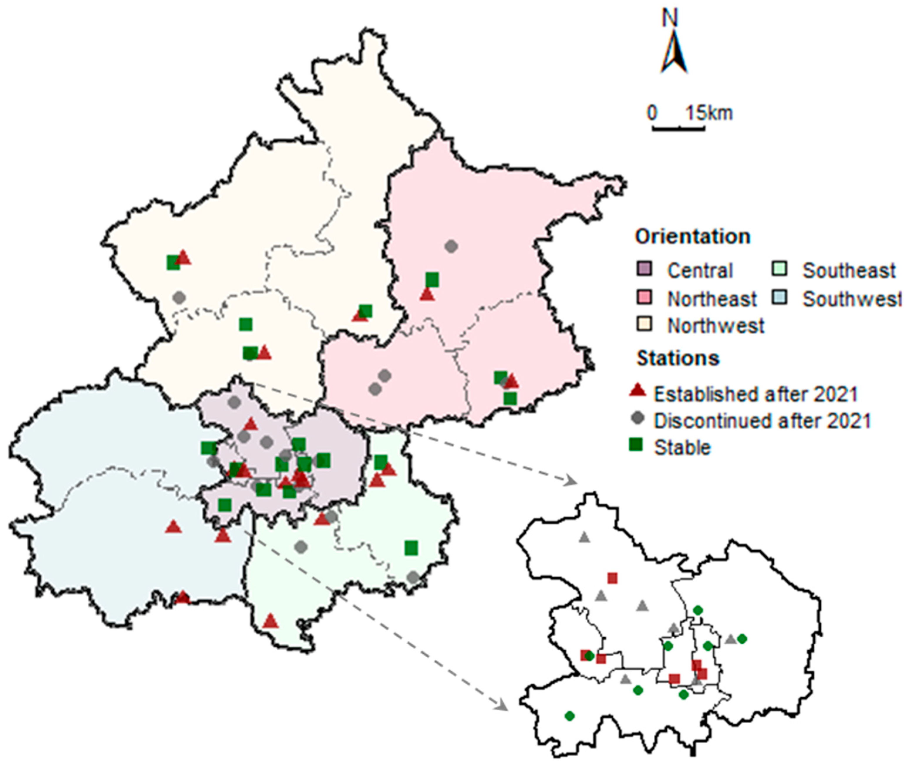
2.2.1. Ground-Level Ozone Concentration

Ground-level ozone concentration data are sourced from the Beijing Environmental Monitoring Centre and can be downloaded publicly from the website (https://quotsoft.net/air/) (accessed on 5 November 2024). The locations of ozone monitoring stations are shown in Figure 2. The monitoring network in the Beijing region includes 35 stations, covering both urban built-up areas and surrounding rural and suburban regions. The stations are classified into five types based on geographic positioning. Monitoring stations in urban areas are spread across the six central administrative districts of Beijing—Haidian, Chaoyang, Dongcheng, Xicheng, Fengtai, and Shijingshan—referred to collectively as the “Central”. Additionally, suburban monitoring stations in the suburbs are grouped into four areas: northeast, northwest, southeast, and southwest.
We retrieved hourly average ozone concentrations for the period from 2014 to 2023 from 35 monitoring stations across Beijing. Ozone concentrations were measured using ultraviolet absorption spectrometry and differential optical absorption spectroscopy, in accordance with the Chinese Environmental Protection Standards HJ 193-2013, and were validated following the Technical Guidelines [41]. To ensure data reliability and to account for anomalies potentially induced by COVID-19 control measures, we applied a comprehensive data-cleaning procedure. This procedure was designed to address unreliable outliers, such as sudden spikes in the data [42]. Initially, all hourly data from each monitoring site were standardized. Data points were flagged as outliers and removed if their standardized value exceeded 4 or if they were 9 times higher than the preceding hour’s value. Additionally, in compliance with the Chinese National Ambient Air Quality Standards (CNAAQS), missing or invalid data were excluded. Specifically, we omitted data from stations that reported fewer than 20 valid hours per day, fewer than 27 valid days per month (25 days for February), or fewer than 324 valid days per year when calculating the annual average ozone concentrations. After the cleaning process, the percentage of valid hourly ozone data at each monitoring station consistently remained at or above 97%.

2.2.2. Satellite-Derived Ozone Concentration

To estimate the spatial continuity of ozone distribution, we used the MDA8 values from the ChinaHighO3 dataset. This dataset is a subset of the broader China High-Resolution Air Pollutants (CHAP) dataset, which is publicly accessible at https://nnu.geodata.cn/featured_data.html (accessed on 5 November 2024). The ChinaHighO3 dataset integrates multiple data sources, including ground-based ozone monitoring observations, satellite remote sensing products, atmospheric reanalysis data, and emission inventories. By synthesizing these diverse datasets, this dataset provides high-resolution ozone concentration estimates with a spatial resolution of 1 km across China. This enables detailed and precise assessments of ozone exposure, even in areas lacking direct monitoring coverage. The dataset has been rigorously validated and has demonstrated high accuracy in estimating daily ozone levels. Key performance metrics include a cross-validation coefficient of determination (CV-R²) of 0.87, a root mean square error (RMSE) of 17.10 µg/m3, and a mean absolute error (MAE) of 11.29 µg/m3 at the daily scale [43,44].

2.2.3. Population Data

High-resolution population data with a spatial resolution of 1 km for each year from 2014 to 2023 was obtained from the LandScan global population database (https://landscan.ornl.gov/) (accessed on 5 November 2024). LandScan provides high-resolution estimates of population distribution at the grid cell level, utilizing a combination of satellite imagery, land cover data, census data, and other geospatial information. Figure 3 shows the averaged gridded population data from 2014 to 2024 for Beijing as derived from LandScan. To align the LandScan population data with official statistics, we performed year-by-year adjustments using data from the Beijing Statistical Yearbook (https://nj.tjj.beijing.gov.cn/nj/main/2022-tjnj/zk/indexeh.htm) (accessed on 5 November 2024). The yearbook provides authoritative population counts, including the total population of residents in the city and detailed counts for each of Beijing’s 16 districts. The adjustment process ensured consistency between LandScan’s gridded data and the official demographic information reported for Beijing. By calibrating the population estimates at the district level, we improved the reliability and applicability of the population data for spatial analysis and health impact assessments.

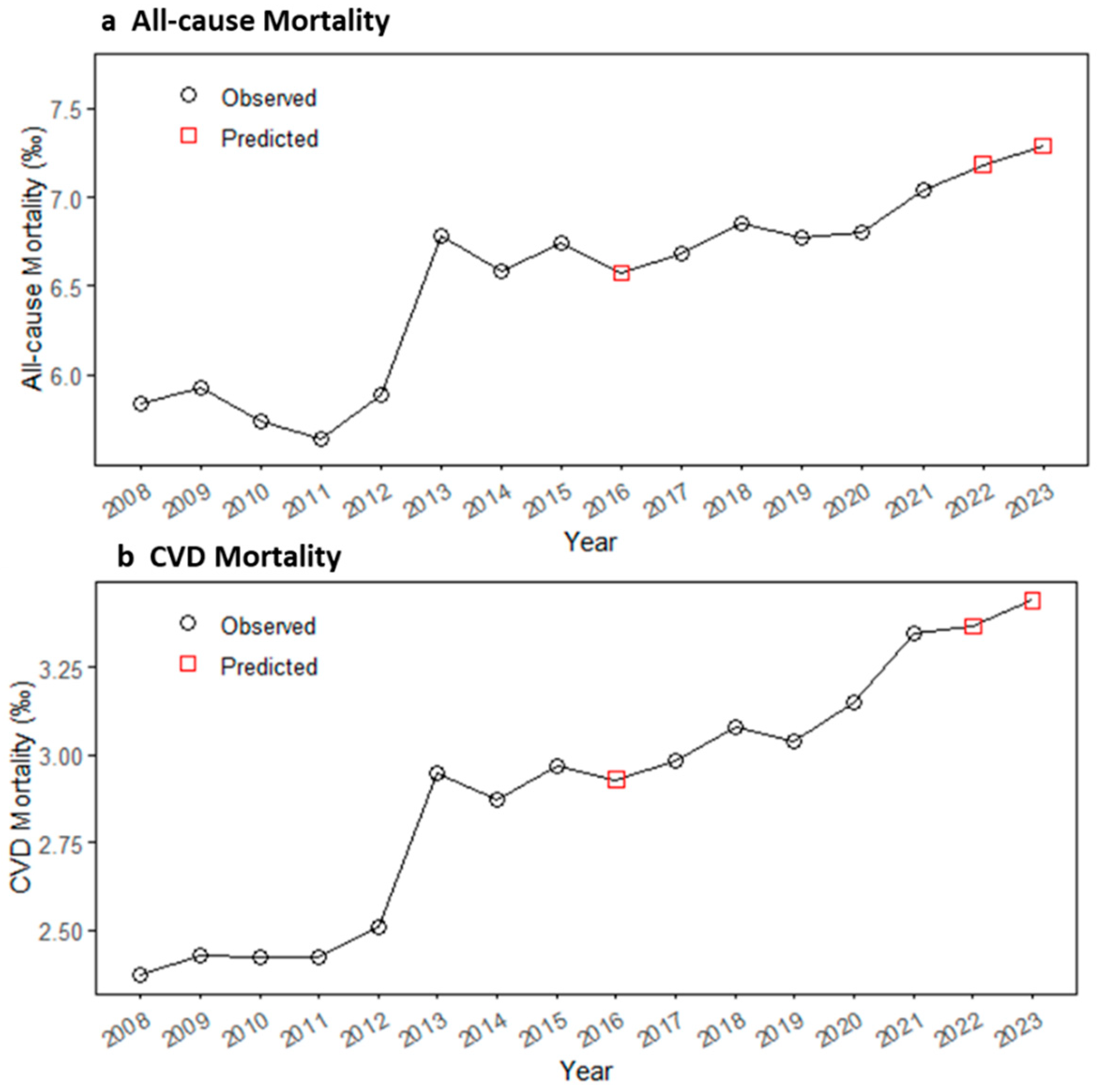
2.2.4. Baseline Mortality Data

Baseline mortality data were obtained from the Chinese Center for Disease Control and Prevention, which provides long-term cause-specific mortality surveillance datasets (2008–2021; https://ncncd.chinacdc.cn/jcysj/siyinjcx/syfxbg/; accessed on 5 November 2024). We utilized regional mortality data, including data from Beijing, to ensure geographic representativeness. Two primary health outcomes were analyzed: all-cause mortality (A00-R99) and cardiovascular mortality (I00-I99), which is consistent with previous studies [45,46]. Here, mortality is defined as the number of people whose deaths are attributable to ozone exposure. The coding of mortality data follows the International Classification of Diseases [47]. While the study period covers 2014–2023, gaps in the dataset for 2016, 2022, and 2023 were addressed using linear regression interpolation (R² = 0.92). This approach ensured temporal continuity while minimizing bias from missing data. The results are shown in Figure 4.

2.2.5. Concentration–Response Relationship Data

The concentration–response relationship data used in studies on the effects of ozone pollution on human health are based on previous cohort studies [45,48], which can be challenging to obtain for specific regions due to the significant human and material resources required. Table 1 summarizes the relative risk (RR), which is the concentration–response coefficient for ozone exposure in the published literature in China. We used the overall RR value reported in the Yin et al. (2017) [45], as the city-specific RR for Beijing was not explicitly provided. We selected the RR from this study because it conducted a comprehensive investigation and provided estimates for both types of health endpoints (all-cause mortality and cardiovascular mortality) in megacities across China.

2.3. Ozone Metric Determination

Table 2 summarizes the ozone-related indicators used in this study. Regarding the analysis of ozone pollution in Beijing, the indicators are selected in accordance with the principles outlined in the Environmental Air Quality Standards of China (GB 3095–2012). Two types of ozone concentration indicators were used: the one-hour ozone concentration (1 h ozone) and the MDA8. These indicators fulfill the requirements of air quality assessment and correspond to the Chinese national air quality classification method for ozone pollution (Table 3). For the health impact assessment, the MDA8 value was chosen to generate population exposure concentration. The MDA8 metric is consistent with the study from which the RR was derived [45].
The quality control of raw data obtained from the environmental monitoring platform is performed through the following steps: (1) Removal of data with hourly average concentrations less than or equal to zero and missing data. (2) Removal of 8 h running average concentrations if they contain fewer than 6 h of valid data. (3) If the number of valid 8 h average concentration values is less than 14 for a day and the MDA8 does not exceed the concentration limit standard (100 μg/m3) for that station, the ozone concentration assessment value for that day at the monitoring station is removed. (4) If the number of valid daily maximum 8 h ozone concentration averages is less than 27 in a month (25 in February), the ozone concentration assessment value for that month at the monitoring station is removed. (5) If the number of valid daily maximum 8 h ozone concentration averages is less than 324 in a calendar year, the annual evaluation value for ozone concentration at the monitoring station for that year is considered invalid.

2.4. Ozone Exposure Estimates

We applied two methods to estimate the spatial distribution of ozone exposure and its associated health impacts. The first method utilizes spatially continuous ozone concentration data from the ChinaHighO3 dataset, which integrates ground-based observations, remote sensing products, atmospheric reanalysis data, and emission inventories to generate high-resolution ozone estimates. These estimates are provided at a fine spatial resolution of 1 km, enabling detailed analysis of ozone exposure across both urban and rural areas, including regions without monitoring stations. The second method adopts a district-based interpolation approach, which aggregates ozone concentration data from monitoring stations within defined administrative districts. Using this method, ozone concentrations are averaged or interpolated based on the station-level data available within each district, providing an alternative perspective on exposure distribution. This district-based aggregation reflects the localized influence of monitoring coverage and allows for direct comparisons at the administrative level. By employing both methods, we aim to compare and evaluate the variability and sensitivity of health impact estimates to differences in spatial resolution and data sources of ozone concentration.

2.5. Ozone Health Impact Assessment

The formulas used for estimating ozone health impacts originate from epidemiological studies on air pollution [23,24,25]. The log-linear model, widely used in health risk assessments, links pollutant exposure to relative risk based on concentration changes. MDA8 was selected for health assessments due to its significant correlation with all-cause, respiratory, and circulatory mortalities in epidemiological studies [59]. Developed by environmental health researchers and applied by organizations like the WHO, this model calculates mortality by relating ozone levels to population exposure and baseline mortality rates [8,14,33]. The equation for the log-linear model is as follows:
R R = e β   C
Δ M o r t a l i t y = y 0 × R R 1 R R × P o p = y 0 × ( 1 1 exp β C C 0 ) × P o p
where ΔMortality is the total number of deaths attributed to exposure to ozone resulting in the specific health endpoint in 2022. The relative risk (RR) is the concentration–response coefficient. C represents the change in concentration when defining the RR. C represents the current ozone concentration, and C 0 represents the threshold concentration, below which the health risk associated with ozone exposure is considered negligible or insignificant. Pop is the population exposed to ozone pollution, and y0 represents the baseline mortality rate. The parameter β is the relative risk.
From a public health perspective, this study evaluated two scenarios based on China’s tiered air quality standards of ozone MAD8 concentration (Grade I: 100 μg/m3; Grade II: 160 μg/m3). We compare annual avoidable mortality under the assumption of effective pollution control, where concentration changes are calculated as the difference between baseline and controlled ozone levels. The baseline of spatially continuous ozone concentration surface was derived from satellite data, while the controlled scenario was generated by reducing excessive ozone concentrations to comply with the stricter Grade I (100 μg/m3) or Grade II (160 μg/m3) standards. The assumed control strategy aligns with China’s national standards, enabling the quantification of mortality reductions attributable to ozone mitigation. These calculated reductions reflect the potential health benefits achievable through stricter air pollution control measures.

3. Results

3.1. Temporal Patterns of Ozone

By applying station-based observations of ozone concentration during the past decade (from 2014 to 2023), we revealed significant diurnal variations, seasonal dynamics, and long-term changes (pre- and post-pandemic) in ozone pollution in Beijing.

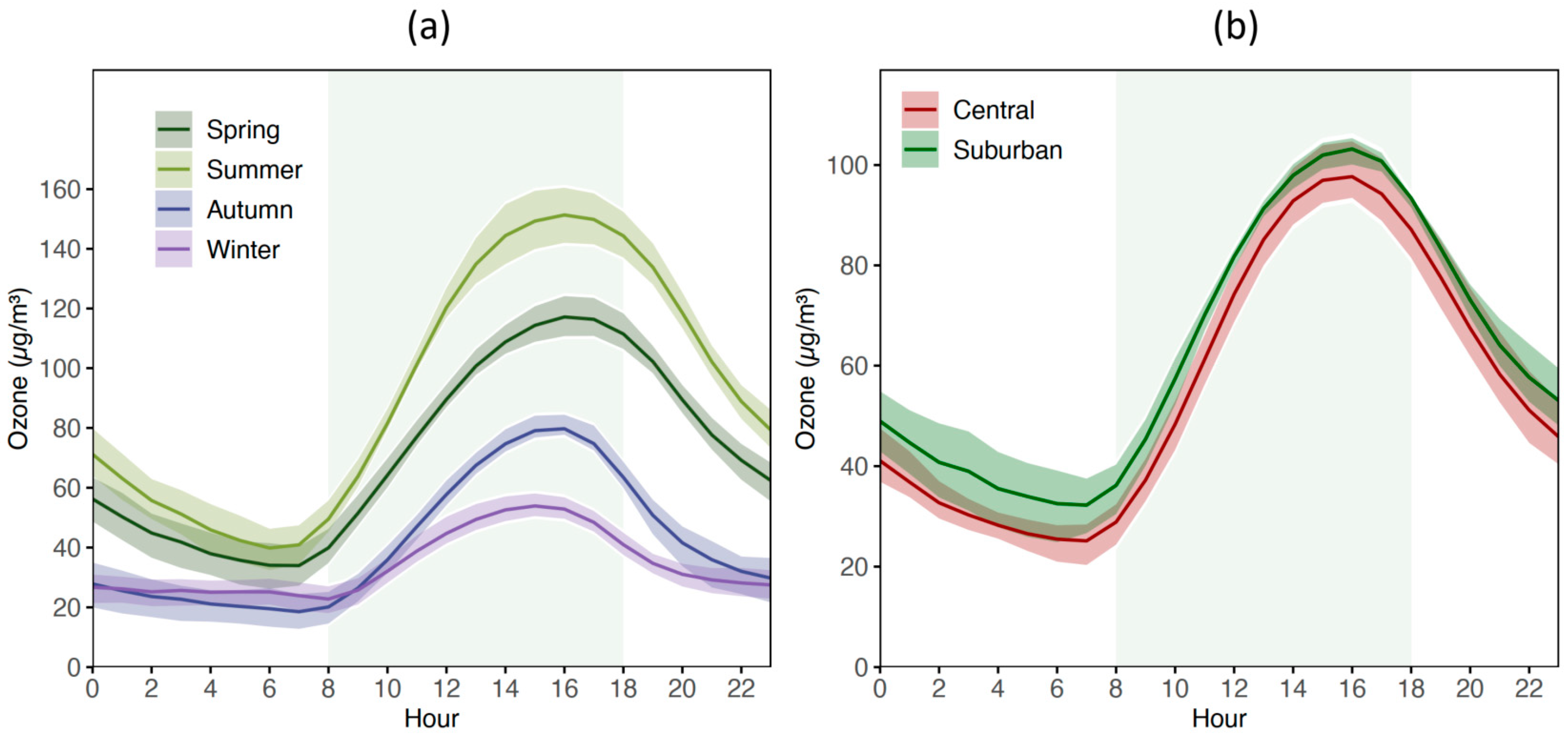
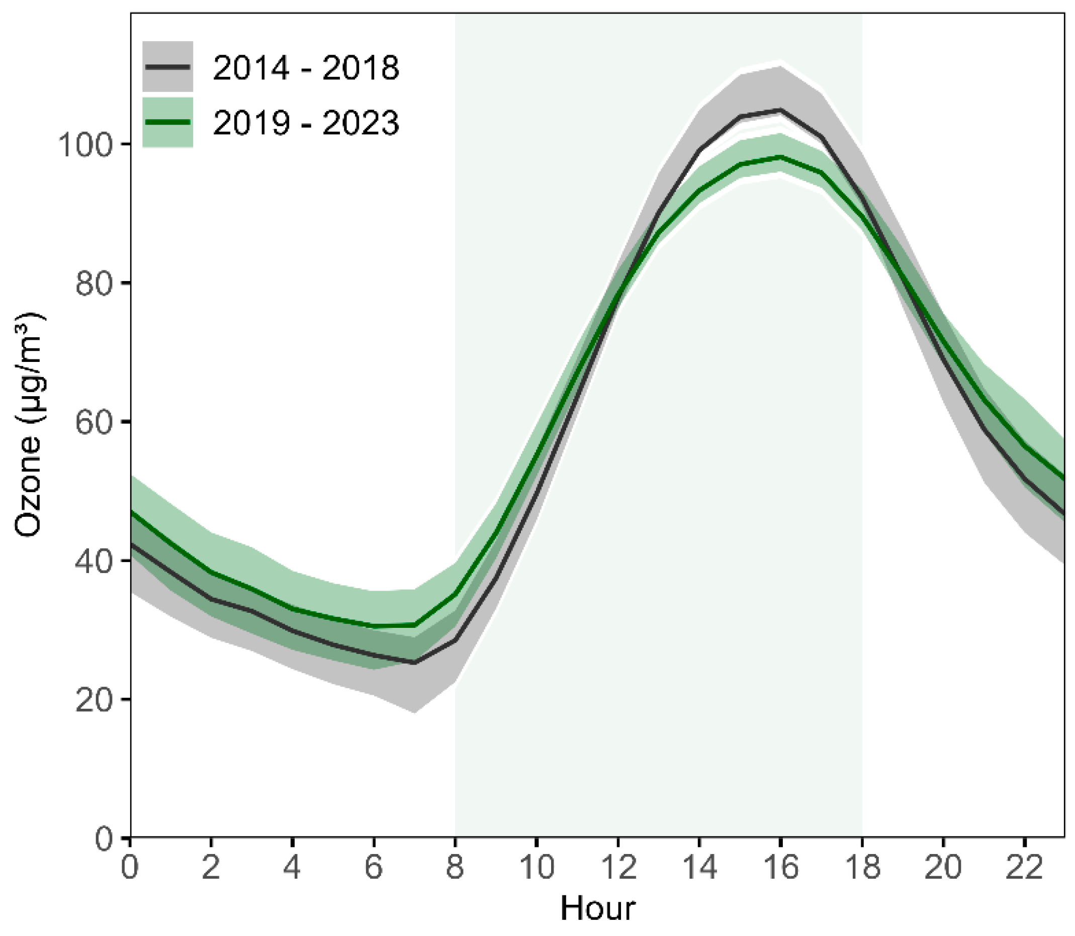
3.1.1. Diurnal Variations in Hourly Ozone Concentration

As shown in Figure 5, we assessed the diurnal variations in surface ozone concentrations in Beijing by seasons and regions. In general, ozone concentrations exhibit a typical diurnal cycle, with an upward trend during the sunlight radiation period. Figure 5a presents the hourly ozone pattern across the four seasons. During warm seasons (spring and summer), ozone concentrations show high-amplitude fluctuations throughout the day, with a peak of 151.34 μg/m3 in summer and 117.16 μg/m3 in spring, and a fluctuation range exceeding 100 μg/m3. The data dispersion, measured by interquartile range (IQR) at the peak period in summer, approaches 20 μg/m3. In autumn, the curve shows a transitional pattern. The day–night concentration difference reduces to 56 μg/m3, and the daytime ozone level peaks at 79.7 μg/m3 with a lower variability. The winter curve is nearly flat, with ozone concentrations remaining between 22.8 and 53.9 μg/m3 throughout the day. The timing of the ozone peak is synchronized with the changing of daylight hours, as the winter peak occurs about 1 h earlier than it does in summer. Spatially, Figure 5b further compares the diurnal variation in ozone between the urban and suburban areas. The ozone patterns are largely consistent across both regions. However, the average ozone concentration is slightly higher in the suburbs than in the urban core, with a difference of 5.0–8.9 μg/m3. In addition, the urban sites record greater variability in the central values during the daytime period (12:00–18:00), particularly at higher concentration levels. However, suburban sites exhibit increased variability during nighttime hours (00:00–06:00). At the peak concentration period (16:00), the third quartile values for both urban and suburban areas converge at approximately 105 μg/m3, indicating a diminished urban–rural concentration gradient under extreme ozone events.
To investigate the long-term trend of ozone concentrations in Beijing, we divided the study period into two consecutive five-year intervals: 2014–2018 and 2019–2023. These periods also represent ozone levels before and after the COVID-19 pandemic, allowing for an assessment of potential shifts in atmospheric composition and pollution dynamics. As shown in Figure 6, the diurnal cycle of ozone is consistent across both periods, while differences are observed in the magnitude of ozone concentrations. During the daytime hours (12:00–18:00), ozone concentrations in the post-pandemic period (2019–2023) are consistently lower than those in the pre-pandemic period (2014–2018). Specifically, the peak ozone concentration decreased from 104.9 μg/m3 (2014–2018) to 98.1 μg/m3 (2019–2023), a reduction of approximately 6.8 μg/m3. The average ozone concentration during this period also decreased by approximately 4.2 μg/m3. Conversely, in the early morning hours (00:00–06:00), ozone concentrations are higher in the post-pandemic period, with an average increase of 5.4 μg/m3 compared to the pre-pandemic period.

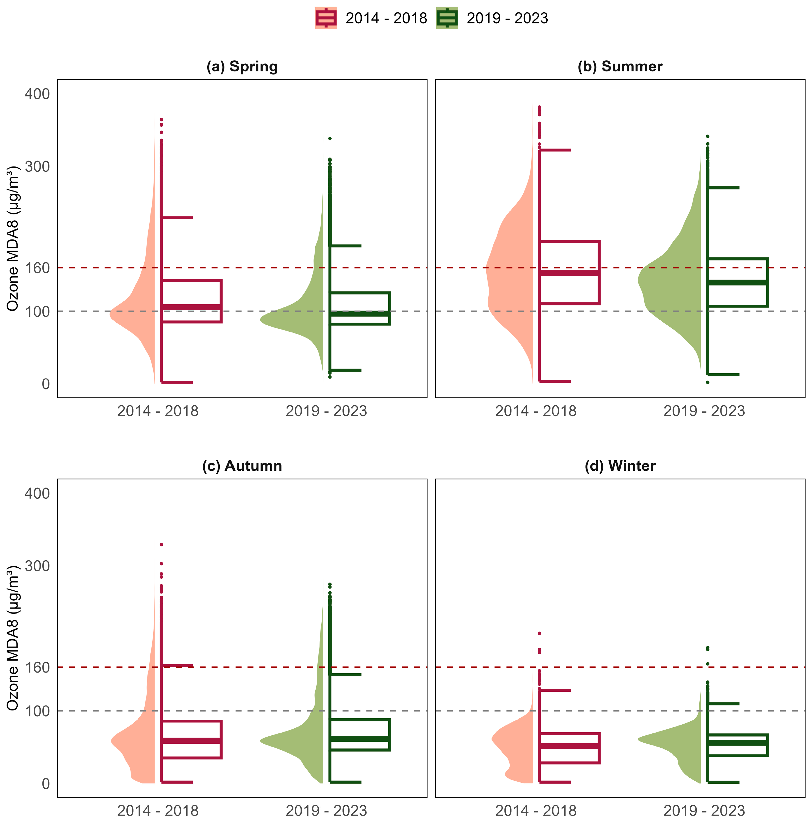
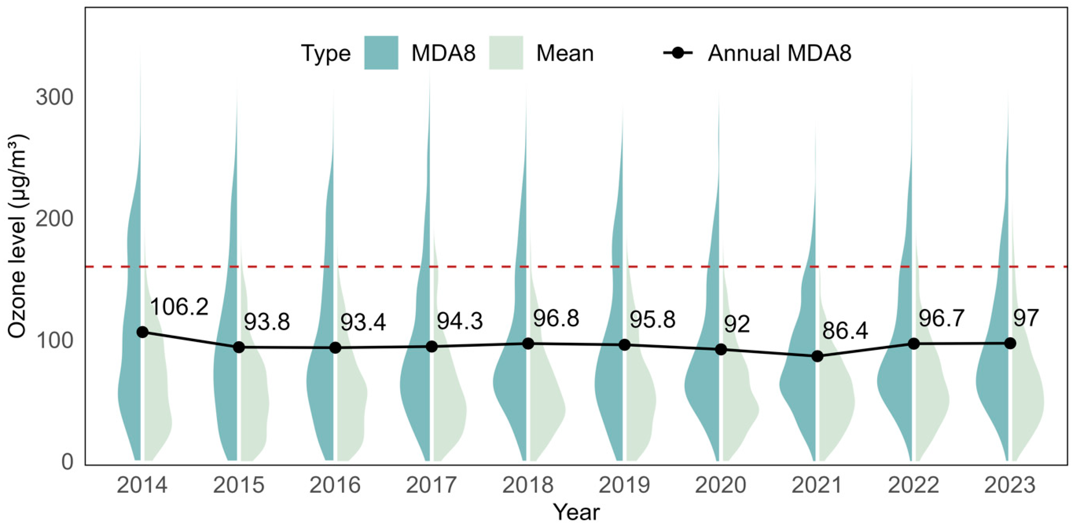
3.1.2. Seasonal and Annual Variations in Daily Ozone Concentrations

Figure 7 presents the distribution of daily ozone concentrations across different seasons derived from monitoring station measurements. On the seasonal scale, ozone concentrations are significantly higher during the warm seasons (average 113.46 μg/m3 in spring and 148.67 μg/m3 in summer), compared to colder seasons (70.76 μg/m3 in autumn and 50.88 μg/m3 in winter). The median ozone MDA8 in spring fluctuated from 96.51 μg/m3 in the earlier period (2014–2018) to 103.88 μg/m3 in the later period (2019–2023), remaining close to the Grade I air quality standard (Figure 7a). A similar trend is observed in summer (Figure 7b), where the median MDA8 ozone concentration decreased from 153.10 μg/m3 to 141.50 μg/m3. In contrast, autumn and winter show relatively minor changes in ozone levels (Figure 7c,d). Simultaneously, across all seasons, a narrowed IQR could be observed, especially in warmer seasons. These reductions suggest a stabilization of high ozone episodes over time.
To investigate long-term variations in ozone pollution in Beijing, we assessed the annual averaged MDA8 level and its distribution based on the station observations of each year from 2014 to 2023 (Figure 8). The annual mean MDA8 fluctuated from 106.2 μg/m3 in 2014 to 97 μg/m3 in 2023, with an insignificant trend. The distributions of MDA8 (left, dark green) and mean daily ozone (right, light green) reveal that the proportion of days with high-level ozone concentrations (MDA8 exceeding the Grade II threshold of 160 μg/m3, denoted as the red dashed line) is slightly decreased, with a more concentrated distribution at a moderate level.

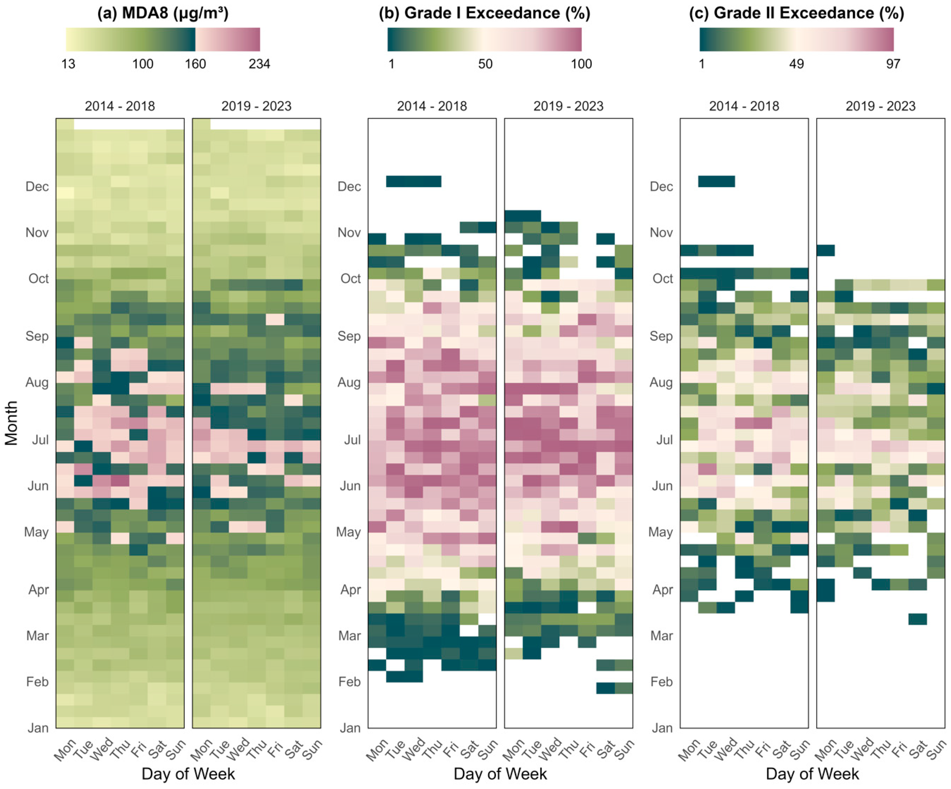
3.1.3. Compliance with Air Quality Standards

Figure 9 shows the changes in daily ozone levels and exceedance rates between the pre-pandemic (2014–2018) and post-pandemic (2019–2023) periods. The comparison in Figure 9a shows a clear downward trend in summer ozone concentrations, with a decreased proportion of high-level ozone in the post-pandemic period. Specifically, during the summer months (June–August), the proportion of days exceeding 160 μg/m3 decreased from 48.4% in the pre-pandemic period to 25.5% in the post-pandemic period. Figure 9b shows the probability of ozone concentrations exceeding Grade I air quality standards on the given day of year. We find the probability of exceedances shows little difference between the two periods, with an average of 81.49% (pre-pandemic) and 80.34% (post-pandemic) in summer. However, the probability of Grade II exceedances (Figure 9c) decreased during the post-pandemic period, especially in the summer months, with a reduction of 12.80% on the seasonal average.

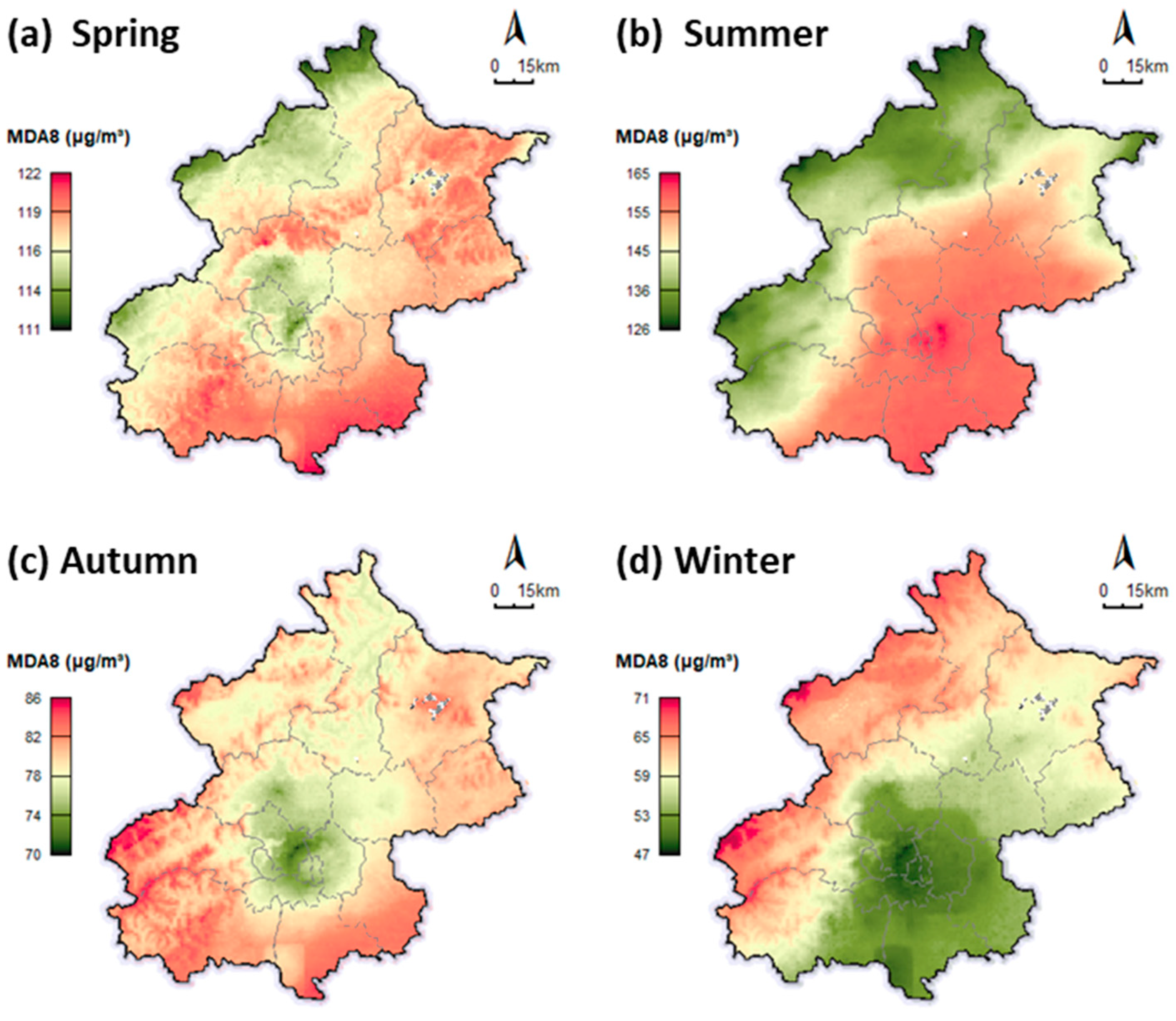
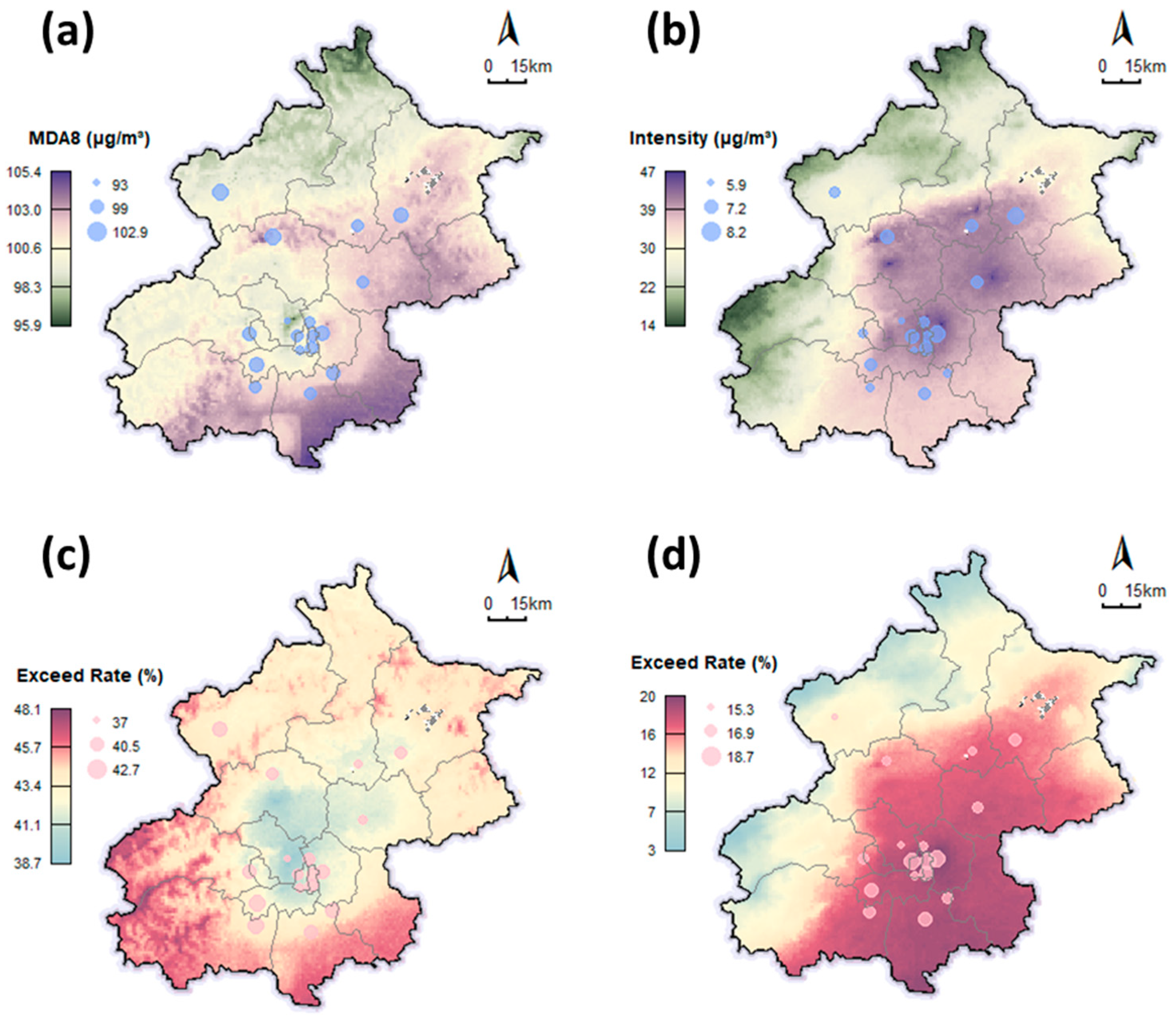
3.2. Spatial Distribution of Ozone Pollution

Using spatially continuous satellite-derived ozone data, we assess the spatial distribution characteristics of ozone across the Beijing region. Figure 10 presents the spatial patterns of the mean MDA8 levels over the entire study period. In spring (Figure 10a), high-concentration zones (>119 μg/m3) are mainly observed in the southeastern plains (Daxing and Tongzhou districts) and along the transitional belt between plains and mountainous terrain, forming a ring-like structure encircling the lower-concentration region in the northwest part of the central urban area (Shijingshan and Haidian districts). The elevated terrain (Yanshan and Western Hills) in the northwestern boundary exhibits the lowest ozone level in spring while still exceeding the Grade I standard. In summer (Figure 10b), the spatial pattern of ozone reveals a distinct northwest-to-southeast gradient, aligning with the mountain–plain topographic division of Beijing. The central urban regions become a strong pollution core (>161.0 μg/m3), with elevated concentrations extending over the entire south plain (153–165 μg/m3). The ozone concentration shifts rapidly across a narrow zone and then disperses more evenly in the northern and western mountainous regions at relatively low levels (141.0–125.8 μg/m3). In autumn (Figure 10c), the ozone distribution shows a transitional character with a typical ring-like pattern. The central urban core area accumulates relatively less ozone, while its concentration gradually increases in the surrounding areas, especially along the southern boundary, where the levels are within a higher range (83–86 μg/m3). In winter (Figure 10d), while a typical northwest-to-southeast gradient is observed, the relationship is reversed compared to summer. The lowest pollution occurs in urban ozone, with relatively higher concentrations in mountainous regions.
Figure 11 presents the spatial distribution characteristics of key ozone pollution indicators, including the multi-year averaged MDA8 (a) and average pollution intensity (b) values, along with the exceedance rates of Grade I (c) and Grade II (d), revealing significant patterns of ozone pollution differentiation.
In Figure 11a, the satellite-derived ozone data reveal that over the past decade, the mean annual ozone MDA8 values are higher in the southern area, with a gradual decline toward the northwest. Meanwhile, a low-value center is observed in the northern part of the central urban area with ozone concentrations lower than 100 µg/m3. The variation in annual MDA8 concentrations across different regions is approximately 10 μg/m3, reflecting a moderate spatial heterogeneity in ozone distribution. In comparison, the station-based monitoring data show a similar spatial pattern, with annual mean MDA8 differences across the monitoring sites remaining within 10 µg/m3. The lowest ozone concentrations are observed in Haidian district at 93.00 µg/m3, aligning with the low-value center in the northern urban area that was identified by the satellite-derived data. However, the sparse distribution of monitoring stations in suburban areas limits their ability to capture finer-scale spatial variations. Figure 11b shows the spatial distribution of the average intensity of ozone pollution events, quantified by the portion of ozone MDA8 concentrations exceeding the Grade II standard. The areas with the most intense ozone pollution are located in the central and southern regions, with the mean ozone intensity exceeding 47 µg/m3. While in the northwestern mountainous area, the intensity is much lower, with a minimum of 14 µg/m3. The pollution intensity recorded by the monitoring stations ranges from 5.9 µg/m3 to 8.2 µg/m3, which is lower and more restricted compared to the intensity distribution retrieved from the satellite data.
Figure 11c indicates that the exceedance rate in the central urban cluster is generally lower than that in the surrounding suburban areas. The highest exceedance rates are concentrated in the southern region, forming a ring-like gradient band closely coupled with the pattern of ozone levels in the two transitional seasons (spring and autumn). Monitoring data revealed that the highest exceedance rate (42.7%) was recorded in the southern region, whereas the northern and central urban areas exhibited relatively lower rates (37–41.1%). The exceedance rates observed across monitoring stations show a narrower variation compared to the values from the remote sensing data (48.1–38.7%), along with a lower mean exceedance rate (−3.6% relative to the remote sensing estimates). The Grade II exceedance in Figure 11d presents a different spatial distribution, with a distinct increasing gradient from the northwest mountainous region to the southeast plain. The highest exceedance rates, reaching 20.26%, are concentrated in the central urban area (Dongcheng and Chaoyang districts), forming the core of high exceedance values. The surrounding southeastern lowlands also exhibit elevated exceedance rates, ranging between 15.3% and 16.9%, while in the northwestern mountainous region, the exceedance rates are lower than 7%. The highest monitored exceedance rates are observed in the central urban core and southeastern lowlands, aligning with the high-exceedance zones identified by the satellite data. However, monitoring sites record weaker spatial heterogeneity, with a range of 15.3–18.7%, when compared to satellite-based data (3.0–20.3%).

3.3. Avoidable Mortality Under Tiered Air Quality Standards

Based on the Chinese National Environmental Air Quality Assessment Standard graded management system (Grade I: 100 μg/m3; Grade II: 160 μg/m3), we estimated ozone-related health benefits from 2014 to 2023 by estimating avoidable mortality under both standards.
As shown in Figure 12a, implementing the Grade II standard would reduce an annual mean of 165 all-cause deaths (95% CI: 91–235), accounting for approximately 0.56% of the total population. In contrast, adherence to the stricter Grade I standard could prevent 576 deaths annually (95% CI: 317–827), representing a 3.5-fold increase in health benefits. For cardiovascular disease (CVD) mortality (Figure 12b), the Grade II and Grade I scenarios correspond to 84 (95% CI: 32–132) and 294 (95% CI: 111–467) avoidable deaths per year, respectively. From a temporal perspective, the health benefit trends for both standards are similar. Since 2014, excess mortality from ozone pollution has continuously risen, peaking in 2019. The excess all-cause deaths due to ozone levels exceeding both Grade I and II air quality standards were 714 and 248 on average in 2019 (Figure 12a), respectively. From 2020 to 2021, the health benefit declined in parallel, with the Grade I scenario dropping to 435 and the Grade II scenario dropping to 74. However, after 2022, the benefits for both standards rebounded, reaching 662 (Grade I) and 201 (Grade II) in 2023, similar to the peak levels observed in 2019. Spatially, we find the ozone-related excess mortality highly correlates with population density, peaking in urban centers like Chaoyang and Haidian districts due to heightened exposure. These densely populated areas would benefit most from achieving ozone pollution control compliance.
The spatial patterns of avoidable all-cause mortality are shown in Figure 13. According to the cumulative avoidable all-cause death density under Grade II air quality compliance (160 μg/m3) over the 10-year period (Figure 13a), the highest cumulative avoidable death density occurred in the central urban area, with values reaching up to 3.4 persons per grid, corresponding to the core districts (Dongcheng, Xicheng, Chaoyang, and Haidian). The density decreased to around 1.7 persons per grid in inner suburban areas, including parts of Fengtai and Shijingshan districts. This spatial pattern of avoidable death density is identical to population density, highlighting the role of population concentration as a primary driver of avoidable mortality. We further evaluated the incremental health benefits associated with achieving different air quality standards, quantified as the proportion of avoidable deaths under the Grade II standard (160 µg/m3) relative to those attainable under the stricter Grade I standard (100 µg/m3), as shown in Figure 13b. It is suggested that compliance with the Grade II standard can achieve up to 33.5% of the health benefits, in terms of avoidable mortality, that would be realized under the Grade I threshold, especially evident in the core urban districts. This modest difference in health outcomes between Grade II and Grade I in core areas could further support the implementation of tiered air quality standards in Beijing, as it allows flexibility to prioritize stricter standards in suburban zones, while focusing on achievable gains in the urban core. In urban settings, targeting Grade II can deliver substantial health benefits without the immediate pressure of meeting a more resource-intensive standard, balancing the need to safeguard public health with the realities of implementation.

4. Discussion

Our study highlights significant patterns of ozone pollution and related health impacts in Beijing. The diurnal and seasonal patterns are consistent with previous research in Beijing and other regions [33,36,37,38,40,42,60]. Specifically, we observed distinct diurnal variations in ozone pollution, matching the patterns found in other studies. Beijing’s hourly ozone concentrations typically rise during daylight, peaking in the afternoon, and drop at night. Studies from Cairo (Egypt) [61], Mongolia [62], Malaysia [63], and other regions [40,60] show similar midday peaks, driven by photochemical reactions under sunlight. Ozone concentrations are driven by photochemical reactions involving NO2 precursors, elevated temperatures, and solar radiation intensity, resulting in diurnal peaks during midday hours when sunlight is most pronounced [10]. Beijing’s severe summer ozone pollution results from its strong dependence on temperature and sunlight, driving higher concentrations in summer and lower levels in winter. These seasonal trends align with previous studies from other countries [18,64].
Our pre-pandemic versus post-pandemic comparative analysis yields novel insights into ozone pollution patterns in Beijing from 2014 to 2023. Previous studies have shown that ozone concentrations responded differently to the COVID-19 lockdowns [65,66,67]. During the COVID-19 lockdown (January to April 2020 in Beijing), strict measures reduced industrial and traffic activities, altering precursor emissions and influencing ozone levels [66]. Previous studies find that ozone levels decreased in the southern China, while in northern China, including the Beijing area, reduced NOx emissions resulted in higher ozone concentrations during the COVID-19 outbreak [65,66,67]. Amplified ozone pollution during the COVID-19 lockdown was also observed in a previous study in different counties [68], reflecting lockdown-related emission changes. We find that the post-pandemic period (2019–2023) saw a reduction in daytime ozone concentrations relative to pre-pandemic levels (2014–2018), but nighttime concentrations increased, suggesting complex precursor emission patterns. Seasonally, ozone declines were pronounced in spring and summer, aligning with reduced precursor emissions during warmer months. Conversely, autumn and winter exhibited few ozone level changes. This underscores the need for dynamic adjustments to address shifting seasonal trends (e.g., the post-pandemic ozone increases in autumn/winter).
China’s tiered air quality standards designate Grade I (100 μg/m3) for ecologically sensitive areas like natural reserves and Grade II (160 μg/m3) for urban functional zones, including residential, industrial, and commercial areas. The 60 μg/m3 threshold difference reflects a policy balance between ecological preservation and socioeconomic costs. From 2014 to 2023, we find that adherence to Grade I and Grade II standards cumulatively prevented 5760 and 1649 deaths, respectively. Tightening standards to align with Grade I thresholds could avoid an additional 4111 deaths, highlighting the health benefits of stricter controls. Economically, Grade I implementation reduced medical burdens by reducing annual healthcare expenditures and mitigating urban productivity losses.
Our study highlights the urgency of addressing ozone pollution and its health impacts in Beijing, China, but it also has limitations that point to important future research directions. First, our analysis focuses on ozone patterns before and after the COVID-19 pandemic but does not explore the underlying causes and mechanisms. The complex interactions between meteorological conditions and emissions, as well as the impacts of policy measures on ozone trends, need further investigation in future studies. Second, the use of a single relative risk value may not capture variations in population responses. Future research could incorporate district-specific epidemiological studies to derive local health impact functions, which would enhance the accuracy of ozone exposure assessments. Lastly, this study does not account for differences in breathing patterns and physical activity levels across different population groups, which could influence individual exposure to ozone pollution. Future research should integrate these exposure factors to provide a more accurate assessment of health impacts in Beijing and other regions.
Our study provides important implications by highlighting the need for health-based, season-specific, and region-specific ozone standards. With high ozone pollution in Beijing, policymakers need to create more focused air quality strategies. Ozone control should work with current efforts to reduce primary pollutants, especially given the link between O3 and its precursors. Our findings on the health burden from ozone exposure in Beijing, along with avoidable death estimates, suggest that current ozone limits need to be re-examined. The national standard for MDA8 O3, set at 160 μg/m3, may not be enough to protect public health. In addition, previous studies have identified the elderly and those with existing illnesses as sensitive groups for ozone exposure [33,48]. As China’s population ages, the longer time needed to control ozone means that more vulnerable people will face harmful exposure. This makes it urgent to adopt stronger limits to protect vulnerable people.

5. Conclusions

This study highlights critical insights into ozone pollution in Beijing, emphasizing its spatiotemporal variability, regulatory challenges, and public health implications. Diurnal and seasonal patterns reveal elevated ozone volatility in spring and summer, with post-pandemic shifts exacerbating nighttime concentrations. Spatial analysis uncovers seasonal heterogeneity, particularly in urban cores exceeding air quality thresholds during summer. Health assessments demonstrate that adopting Grade I standards over Grade II could significantly reduce mortality, underscoring the urgent need for revised ozone regulations tailored to densely populated areas. These findings advocate for adaptive, localized pollution control strategies to mitigate exposure risks in Beijing and comparable megacities globally.

Author Contributions

Conceptualization, J.Y. and F.Y.; methodology, software, F.Y.; validation, F.Y., J.Y. and L.G.; formal analysis, F.Y. and J.Y.; investigation, resources, data curation, F.Y.; writing—original draft preparation, F.Y.; writing—review and editing, F.Y., J.Y. and L.G.; visualization, F.Y.; supervision, J.Y.; project administration, J.Y. and L.G. All authors have read and agreed to the published version of the manuscript.

Funding

This study was supported by the National Natural Science Foundation of China (Grant No. 42271030), the Fujian Provincial Funds for Distinguished Young Scientists (Grant No. 2022J06018), and the Natural Science Foundation of Fujian Province (Grant No. 2022J01604).

Institutional Review Board Statement

Not applicable.

Informed Consent Statement

Not applicable.

Data Availability Statement

All data used in this study are publicly available. Ground-level ozone observation data can be downloaded from the website (https://quotsoft.net/air/) (accessed on 5 November 2024). Gridded population data are accessible at (https://landscan.ornl.gov/) (accessed on 5 November 2024). The 2022 Beijing Statistical Yearbook can be found at the official statistical resource (https://nj.tjj.beijing.gov.cn/nj/main/2022-tjnj/zk/indexeh.htm) (accessed on 5 November 2024). Baseline mortality rates are obtained from the Chinese Center for Disease Control and Prevention, available at (https://ncncd.chinacdc.cn/jcysj/siyinjcx/syfxbg/) (accessed on 5 November 2024).

Conflicts of Interest

The authors declare no conflicts of interest.

References

  1. Brauer, M.; Roth, G.A.; Aravkin, A.Y.; Zheng, P.; Abate, K.H.; Abate, Y.H.; Abbafati, C.; Abbasgholizadeh, R.; Abbasi, M.A.; Abbasian, M.; et al. Global Burden and Strength of Evidence for 88 Risk Factors in 204 Countries and 811 Subnational Locations, 1990–2021: A Systematic Analysis for the Global Burden of Disease Study 2021. Lancet 2024, 403, 2162–2203. [Google Scholar] [CrossRef]
  2. Sicard, P.; Agathokleous, E.; Anenberg, S.C.; De Marco, A.; Paoletti, E.; Calatayud, V. Trends in Urban Air Pollution over the Last Two Decades: A Global Perspective. Sci. Total Environ. 2023, 858, 160064. [Google Scholar] [CrossRef] [PubMed]
  3. Zhang, X.; Yan, B.; Du, C.; Cheng, C.; Zhao, H. Quantifying the Interactive Effects of Meteorological, Socioeconomic, and Pollutant Factors on Summertime Ozone Pollution in China during the Implementation of Two Important Policies. Atmos. Pollut. Res. 2021, 12, 101248. [Google Scholar] [CrossRef]
  4. Sicard, P.; Khaniabadi, Y.O.; Leca, S.; De Marco, A. Relationships between Ozone and Particles during Air Pollution Episodes in Arid Continental Climate. Atmos. Pollut. Res. 2023, 14, 101838. [Google Scholar] [CrossRef]
  5. Li, H.; Peng, L.; Bi, F.; Li, L.; Bao, J.; Li, J.; Zhang, H.; Chai, F. Strategy of Coordinated Control of PM2.5 and Ozone in China. Res. Environ. Sci. 2019, 32, 1763–1778. [Google Scholar] [CrossRef]
  6. Zhou, Y.; Yang, Y.; Wang, H.; Wang, J.; Li, M.; Li, H.; Wang, P.; Zhu, J.; Li, K.; Liao, H. Summer Ozone Pollution in China Affected by the Intensity of Asian Monsoon Systems. Sci. Total Environ. 2022, 849, 157785. [Google Scholar] [CrossRef]
  7. Ntourou, K.; Fameli, K.M.; Moustris, K.; Manousakis, N.; Tsitsis, C. Trends of the Global Burden of Disease Linked to Ground-Level Ozone Pollution: A 30-Year Analysis for the Greater Athens Area, Greece. Atmosphere 2024, 15, 380. [Google Scholar] [CrossRef]
  8. Cohen, A.J.; Brauer, M.; Burnett, R.; Anderson, H.R.; Frostad, J.; Estep, K.; Balakrishnan, K.; Brunekreef, B.; Dandona, L.; Dandona, R.; et al. Estimates and 25-Year Trends of the Global Burden of Disease Attributable to Ambient Air Pollution: An Analysis of Data from the Global Burden of Diseases Study 2015. Lancet 2017, 389, 1907–1918. [Google Scholar] [CrossRef]
  9. Nawahda, A.; Yamashita, K.; Ohara, T.; Kurokawa, J.; Yamaji, K. Evaluation of Premature Mortality Caused by Exposure to PM 2.5 and Ozone in East Asia: 2000, 2005, 2020. Water Air Soil Pollut. 2012, 223, 3445–3459. [Google Scholar] [CrossRef]
  10. Seinfeld, J.H.; Pandis, S.N.; Noone, K. Atmospheric Chemistry and Physics: From Air Pollution to Climate Change. Phys. Today 1998, 51, 88–90. [Google Scholar] [CrossRef]
  11. Feng, Z.; De Marco, A.; Anav, A.; Gualtieri, M.; Sicard, P.; Tian, H.; Fornasier, F.; Tao, F.; Guo, A.; Paoletti, E. Economic Losses Due to Ozone Impacts on Human Health, Forest Productivity and Crop Yield across China. Environ. Int. 2019, 131, 104966. [Google Scholar] [CrossRef]
  12. Marco, A.D.; Anav, A.; Sicard, P.; Feng, Z.; Paoletti, E. High Spatial Resolution Ozone Risk-Assessment for Asian Forests. Environ. Res. Lett. 2020, 15, 104095. [Google Scholar] [CrossRef]
  13. De Marco, A.; Garcia-Gomez, H.; Collalti, A.; Khaniabadi, Y.O.; Feng, Z.; Proietti, C.; Sicard, P.; Vitale, M.; Anav, A.; Paoletti, E. Ozone Modelling and Mapping for Risk Assessment: An Overview of Different Approaches for Human and Ecosystems Health. Environ. Res. 2022, 211, 113048. [Google Scholar] [CrossRef]
  14. Zou, B.; You, J.; Lin, Y.; Duan, X.; Zhao, X.; Fang, X.; Campen, M.J.; Li, S. Air Pollution Intervention and Life-Saving Effect in China. Environ. Int. 2019, 125, 529–541. [Google Scholar] [CrossRef]
  15. Wong, D.W.; Yuan, L.; A Perlin, S. Comparison of Spatial Interpolation Methods for the Estimation of Air Quality Data. J. Expo. Anal. Env. Epid. 2004, 14, 404–415. [Google Scholar] [CrossRef]
  16. Sun, Z.; Davis, J.M.; Liu, C.; Gao, W. Spatial Interpolation of Surface Ozone Observations Using Deep Learning. In Proceedings of the of SPIE The International Society for Optical Engineering, San Diego, CA, USA, 19–23 August 2018. [Google Scholar]
  17. Sharif, H.O.; Sunil, T.; Alamgir, H.; Jospeph, J. Application of Validation Data for Assessing Spatial Interpolation Methods for Eight-Hour Ozone or Other Sparsely Monitored Constituents. Environ. Pollut. 2013, 178, 411–418. [Google Scholar] [CrossRef]
  18. Michael, R.; O’Lenick, C.R.; Monaghan, A.; Wilhelmi, O.; Wiedinmyer, C.; Hayden, M.; Estes, M. Application of Geostatistical Approaches to Predict the Spatio-Temporal Distribution of Summer Ozone in Houston Texas. J. Exposure Sci. Environ. Epidemiol. 2019, 29, 806–820. [Google Scholar] [CrossRef]
  19. Shen, L.; Jacob, D.J.; Liu, X.; Huang, G.; Li, K.; Liao, H.; Wang, T. An Evaluation of the Ability of the Ozone Monitoring Instrument (OMI) to Observe Boundary Layer Ozone Pollution across China: Application to 2005–2017 Ozone Trends. Atmos. Chem. Phys. 2019, 19, 6551–6560. [Google Scholar] [CrossRef]
  20. Collet, S.; Kidokoro, T.; Karamchandani, P.; Jung, J.; Shah, T. Future Year Ozone Source Attribution Modeling Study Using CMAQ-ISAM. J. Air Waste Manage. Assoc. 2018, 68, 1239–1247. [Google Scholar] [CrossRef]
  21. Zhao, N.; Pinault, L.; Toyib, O.; Vanos, J.; Tjepkema, M.; Cakmak, S. Long-Term Ozone Exposure and Mortality from Neurological Diseases in Canada. Environ. Int. 2021, 157, 106817. [Google Scholar] [CrossRef]
  22. Finlayson-Pitts, B.J.; Pitts, J.N. Tropospheric Air Pollution: Ozone, Airborne Toxics, Polycyclic Aromatic Hydrocarbons, and Particles. Science 1997, 276, 1045–1051. [Google Scholar] [CrossRef] [PubMed]
  23. Atkinson, R.W.; Yu, D.; Armstrong, B.G.; Pattenden, S.; Wilkinson, P.; Doherty, R.M.; Heal, M.R.; Anderson, H.R. Concentration-Response Function for Ozone and Daily Mortality: Results from Five Urban and Five Rural U.K. Populations. Environ. Health Perspect. 2012, 120, 1411–1417. [Google Scholar] [CrossRef] [PubMed]
  24. Nuvolone, D.; Petri, D.; Voller, F. The Effects of Ozone on Human Health. Environ. Sci. Pollut. Res. 2018, 25, 8074–8088. [Google Scholar] [CrossRef]
  25. Huijbregts, M.A.J.; Hollander, H.A. den et al, V.Z.R. European Characterization Factors for Human Health Damage of PM10 and Ozone in Life Cycle Impact Assessment. Atmos. Environ. 2008, 42, 441–453. [Google Scholar] [CrossRef]
  26. Zou, B.; Wilson, J.G.; Zhan, F.B.; Zeng, Y. Air Pollution Exposure Assessment Methods Utilized in Epidemiological Studies. J. Environ. Monit. 2009, 11, 475–490. [Google Scholar] [CrossRef] [PubMed]
  27. Zu, K.; Liu, X.; Shi, L.; Tao, G.; Loftus, C.T.; Lange, S.; Goodman, J.E. Concentration-Response of Short-Term Ozone Exposure and Hospital Admissions for Asthma in Texas. Environ. Int. 2017, 104, 139–145. [Google Scholar] [CrossRef]
  28. Bae, S.; Lim, Y.H.; Kashima, S.; Yorifuji, T.; Honda, Y.; Kim, H.; Hong, Y.C. Non-Linear Concentration-Response Relationships between Ambient Ozone and Daily Mortality. PLoS ONE 2015, 10, e0129423. [Google Scholar] [CrossRef]
  29. Bell, M.L.; Goldberg, R.; Hogrefe, C.; Kinney, P.L.; Knowlton, K.; Lynn, B.; Rosenthal, J.; Rosenzweig, C.; Patz, J.A. Climate Change, Ambient Ozone, and Health in 50 US Cities. Clim. Change 2007, 82, 61–76. [Google Scholar] [CrossRef]
  30. Kerckhoffs, J.; Wang, M.; Meliefste, K.; Malmqvist, E.; Fischer, P.; Janssen, N.A.H.; Beelen, R.; Hoek, G. A National Fine Spatial Scale Land-Use Regression Model for Ozone. Environ. Res. 2015, 140, 440–448. [Google Scholar] [CrossRef]
  31. Lal, S.; Naja, M.; Subbaraya, B.H. Seasonal Variations in Surface Ozone and Its Precursors over an Urban Site in India. Atmos. Environ. 2000, 34, 2713–2724. [Google Scholar] [CrossRef]
  32. Liu, H.; Liu, S.; Xue, B.; Lv, Z.; Meng, Z.; Yang, X.; Xue, T.; Yu, Q.; He, K. Ground-Level Ozone Pollution and Its Health Impacts in China. Atmos. Environ. 2018, 173, 223–230. [Google Scholar] [CrossRef]
  33. Maji, K.J.; Li, V.O.; Lam, J.C. Effects of China’s Current Air Pollution Prevention and Control Action Plan on Air Pollution Patterns, Health Risks and Mortalities in Beijing 2014–2018. Chemosphere 2020, 260, 127572. [Google Scholar] [CrossRef]
  34. Zhang, M.; Song, Y.; Cai, X. A Health-Based Assessment of Particulate Air Pollution in Urban Areas of Beijing in 2000–2004. Sci. Total Environ. 2007, 376, 100–108. [Google Scholar] [CrossRef] [PubMed]
  35. China: Population Density in Beijing by District 2023. Available online: https://www.statista.com/statistics/1083082/china-population-density-in-beijing-by-district/ (accessed on 25 March 2025).
  36. Ren, J.; Hao, Y.; Simayi, M.; Shi, Y.; Xie, S. Spatiotemporal Variation of Surface Ozone and Its Causes in Beijing, China since 2014. Atmos. Environ. 2021, 260, 118556. [Google Scholar] [CrossRef]
  37. Chen, B.; Yang, X.; Xu, J. Spatio-Temporal Variation and Influencing Factors of Ozone Pollution in Beijing. Atmosphere 2022, 13, 359. [Google Scholar] [CrossRef]
  38. Wang, Z.; Li, J.; Liang, L. Spatio-Temporal Evolution of Ozone Pollution and Its Influencing Factors in the Beijing-Tianjin-Hebei Urban Agglomeration. Environ. Pollut. 2020, 256, 113419. [Google Scholar] [CrossRef] [PubMed]
  39. Chen, Z.; Zhuang, Y.; Xie, X.; Chen, D.; Cheng, N.; Yang, L.; Li, R. Understanding Long-Term Variations of Meteorological Influences on Ground Ozone Concentrations in Beijing During 2006–2016. Environ. Pollut. 2019, 245, 29–37. [Google Scholar] [CrossRef]
  40. Wang, J.; Dong, J.; Guo, J.; Cai, P.; Li, R.; Zhang, X.; Xu, Q.; Song, X. Understanding Temporal Patterns and Determinants of Ground-Level Ozone. Atmosphere 2023, 14, 604. [Google Scholar] [CrossRef]
  41. GB 3095-2012; Ambient Air Quality Standards. Ministry of Ecology and Environment of the People’s Republic of China: Beijing, China, 2012.
  42. Lu, X.; Hong, J.; Zhang, L.; Cooper, O.R.; Schultz, M.G.; Xu, X.; Wang, T.; Gao, M.; Zhao, Y.; Zhang, Y. Severe Surface Ozone Pollution in China: A Global Perspective. Environ. Sci. Technol. Lett. 2018, 5, 487–494. [Google Scholar] [CrossRef]
  43. Wei, J.; Li, Z.; Li, K.; Dickerson, R.R.; Pinker, R.T.; Wang, J.; Liu, X.; Sun, L.; Xue, W.; Cribb, M. Full-Coverage Mapping and Spatiotemporal Variations of Ground-Level Ozone (O3) Pollution from 2013 to 2020 across China. Remote Sens. Environ. 2022, 270, 112775. [Google Scholar] [CrossRef]
  44. Yang, Z.; Li, Z.; Cheng, F.; Lv, Q.; Li, K.; Zhang, T.; Zhou, Y.; Zhao, B.; Xue, W.; Wei, J. Two-Decade Surface Ozone (O3) Pollution in China: Enhanced Fine-Scale Estimations and Environmental Health Implications. Remote Sens. Environ. 2025, 317, 114459. [Google Scholar] [CrossRef]
  45. Yin, P.; Chen, R.; Wang, L.; Meng, X.; Liu, C.; Niu, Y.; Lin, Z.; Liu, Y.; Liu, J.; Qi, J. Ambient Ozone Pollution and Daily Mortality: A Nationwide Study in 272 Chinese Cities. Environ. Health Perspect. 2017, 125, 117006. [Google Scholar] [CrossRef] [PubMed]
  46. Rich, D.Q.; Balmes, J.R.; Frampton, M.W.; Zareba, W.; Stark, P.; Arjomandi, M.; Hazucha, M.J.; Costantini, M.G.; Ganz, P.; Hollenbeck-Pringle, D.; et al. Cardiovascular Function and Ozone Exposure: The Multicenter Ozone Study in oldEr Subjects (MOSES). Environ. Int. 2018, 119, 193–202. [Google Scholar] [CrossRef]
  47. World Health Organization. International Statistical Classification of Diseases and Related Health Problems (ICD). 2019. Available online: https://www.who.int/standards/classifications/classification-of-diseases (accessed on 19 January 2025).
  48. Gao, Q.; Zang, E.; Bi, J.; Dubrow, R.; Lowe, S.R.; Chen, H.; Zeng, Y.; Shi, L.; Chen, K. Long-Term Ozone Exposure and Cognitive Impairment among Chinese Older Adults: A Cohort Study. Environ. Int. 2022, 160, 107072. [Google Scholar] [CrossRef] [PubMed]
  49. Tao, Y.; Huang, W.; Huang, X.; Zhong, L.; Lu, S.E.; Li, Y.; Dai, L.; Zhang, Y.; Zhu, T. Estimated Acute Effects of Ambient Ozone and Nitrogen Dioxide on Mortality in the Pearl River Delta of Southern China. Environ. Health Perspect. 2012, 120, 393–398. [Google Scholar] [CrossRef]
  50. Madaniyazi, L.; Nagashima, T.; Guo, Y.; Pan, X.; Tong, S. Projecting Ozone-Related Mortality in East China. Environ. Int. 2016, 92, 165–172. [Google Scholar] [CrossRef]
  51. Shang, Y.; Sun, Z.; Cao, J.; Wang, X.; Zhong, L.; Bi, X.; Li, H.; Liu, W.; Zhu, T.; Huang, W. Systematic Review of Chinese Studies of Short-Term Exposure to Air Pollution and Daily Mortality. Environ. Int. 2013, 54, 100–111. [Google Scholar] [CrossRef]
  52. Chen, K.; Zhou, L.; Chen, X.; Bi, J.; Kinney, P.L. Acute Effect of Ozone Exposure on Daily Mortality in Seven Cities of Jiangsu Province, China: No Clear Evidence for Threshold. Environ. Res. 2017, 155, 235–241. [Google Scholar] [CrossRef]
  53. Chen, R.J.; Chen, B.H.; Kan, H.D. Health Impact Assessment of Surface Ozone Pollution in Shanghai. China Environ. Sci. 2010, 30, 603–608. [Google Scholar]
  54. Guo, B.; Zhang, Y.; Chen, F.; Deng, Y.; Zhang, H.; Qiao, X.; Qiao, Z.; Ji, K.; Zeng, J.; Luo, B.; et al. Using Rush Hour and Daytime Exposure Indicators to Estimate the Short-Term Mortality Effects of Air Pollution: A Case Study in the Sichuan Basin, China. Environ. Pollut. 2018, 242, 1291–1298. [Google Scholar] [CrossRef]
  55. Wong, C.M.; Qian, Z.; Vichit-Vadakan, N.; Kan, H. Public Health and Air Pollution in Asia (PAPA): A Multicity Study of Short-Term Effects of Air Pollution on Mortality. Environ. Health Perspect. 2008, 116, 1195–1202. [Google Scholar] [PubMed]
  56. Lei, R.; Ding, R.; Zhu, F.; Cheng, H.; Liu, J.; Shen, C.; Zhang, C.; Xu, Y.; Xiao, C.; Li, X.; et al. Short-Term Effect of PM2.5/O3 on Non-Accidental and Respiratory Deaths in Highly Polluted Area of China. Atmos. Pollut. Res. 2019, 10, 1412–1419. [Google Scholar]
  57. Zhong, M.; Saikawa, E.; Chen, F. Sensitivity of Projected PM2.5-and O3-Related Health Impacts to Model Inputs: A Case Study in Mainland China. Environ. Int. 2019, 123, 256–264. [Google Scholar]
  58. Zhang, Q.Q.; Zhang, X.-Y. Ozone Spatial-Temporal Distribution and Trend over China since 2013: Insight from Satellite and Surface Observation. Huanjing Kexue/Environ. Sci. 2019, 40, 1132–1142. (In Chinese) [Google Scholar]
  59. Lefohn, A.S.; Malley, C.S.; Smith, L.; Wells, B.; Hazucha, M.; Simon, H.; Naik, V.; Mills, G.; Schultz, M.G.; Paoletti, E.; et al. Tropospheric Ozone Assessment Report: Global Ozone Metrics for Climate Change, Human Health, and Crop/Ecosystem Research. Elem. Sci. Anth. 2018, 6, 27. [Google Scholar] [CrossRef]
  60. Lyapina, O.; Schultz, M.G.; Hense, A. Cluster Analysis of European Surface Ozone Observations for Evaluation of MACC Reanalysis Data. Atmos. Chem. Phys. 2016, 16, 6863–6881. [Google Scholar] [CrossRef]
  61. Khoder, M.I. Diurnal, Seasonal and Weekdays–Weekends Variations of Ground Level Ozone Concentrations in an Urban Area in Greater Cairo. Environ. Monit. Assess. 2009, 149, 349–362. [Google Scholar] [CrossRef]
  62. Tsydypov, V.V.; Zayakhanov, A.S.; Zhamsueva, G.S.; Balzhanov, T.S.; Dementeva, A.L. Diurnal Variation of Surface Ozone Concentration in the Atmosphere of the Arid Territory of Mongolia, Station Sainshand, in the Warm Period 2005–2014. In Proceedings of the 26th International Symposium on Atmospheric and Ocean Optics, Atmospheric Physics, Moscow, Russia, 6–10 July 2020; Volume 11560, pp. 1377–1380. [Google Scholar]
  63. Awang, N.R.; Elbayoumi, M.; Ramli, N.A.; Yahaya, A.S. Diurnal Variations of Ground-Level Ozone in Three Port Cities in Malaysia. Air Qual. Atmos. Health 2016, 9, 25–39. [Google Scholar] [CrossRef]
  64. Bloomer, B.J.; Vinnikov, K.Y.; Dickerson, R.R. Changes in Seasonal and Diurnal Cycles of Ozone and Temperature in the Eastern U.S. Atmos. Environ. 2010, 44, 2543–2551. [Google Scholar] [CrossRef]
  65. Liu, Y.; Wang, T.; Stavrakou, T.; Elguindi, N.; Doumbia, T.; Granier, C.; Bouarar, I.; Gaubert, B.; Brasseur, G.P. Diverse Response of Surface Ozone to COVID-19 Lockdown in China. Sci. Total Environ. 2021, 789, 147739. [Google Scholar] [CrossRef]
  66. Tong, L.; Liu, Y.; Meng, Y.; Dai, X.; Huang, L.; Luo, W.; Yang, M.; Pan, Y.; Zheng, J.; Xiao, H. Surface Ozone Changes during the COVID-19 Outbreak in China: An Insight into the Pollution Characteristics and Formation Regimes of Ozone in the Cold Season. J. Atmos. Chem. 2023, 80, 103–120. [Google Scholar] [CrossRef] [PubMed]
  67. Chen, Z.; Liu, J.; Cheng, X.; Yang, M.; Shu, L. Stratospheric Influences on Surface Ozone Increase during the COVID-19 Lockdown over Northern China. npj Clim. Atmos. Sci. 2023, 6, 76. [Google Scholar] [CrossRef]
  68. Sicard, P.; De Marco, A.; Agathokleous, E.; Feng, Z.; Xu, X.; Paoletti, E.; Rodriguez, J.J.D.; Calatayud, V. Amplified Ozone Pollution in Cities during the COVID-19 Lockdown. Sci. Total Environ. 2020, 735, 139542. [Google Scholar] [CrossRef] [PubMed]
Figure 1. Geographic location of Beijing and its 16 administrative districts.
Atmosphere 16 00397 g001
Figure 2. Distribution of air quality monitoring stations in Beijing.
Atmosphere 16 00397 g002
Figure 3. The average gridded population data from 2014 to 2023 in Beijing.
Atmosphere 16 00397 g003
Figure 4. Baseline mortality data of all-cause mortality (a) and cardiovascular mortality (b).
Atmosphere 16 00397 g004
Figure 5. Diurnal variation in hourly ozone concentrations by the four seasons (a) and by location (b).
Atmosphere 16 00397 g005
Figure 6. Diurnal variation in hourly ozone concentrations by pre-pandemic period (2014–2018) and post-pandemic period (2019–2023).
Atmosphere 16 00397 g006
Figure 7. Distribution of MDA8 ozone concentrations from the ground monitoring across different seasons, by pre-pandemic (2014–2018) and post-pandemic (2019–2023) periods.
Atmosphere 16 00397 g007
Figure 8. The distribution and variability of maximum daily 8 h average (MDA8) and daily mean ozone concentrations over the years from 2014 to 2023. Black dots represent the annual averaged MDA8 values. The red dashed line represents the Grade II threshold of 160 μg/m3.
Atmosphere 16 00397 g008
Figure 9. Calendar-view patterns of daily ozone levels and exceedance rates between the two periods. (a) The 5-year mean MDA8 (μg/m3), (b) the rate of exceedance compared to the Grade I (100 μg/m3) standard, and (c) the exceedance rate compared to the Grade II standard (160 μg/m3).
Atmosphere 16 00397 g009
Figure 10. Spatial distribution of mean MDA8 ozone concentrations across seasons.
Atmosphere 16 00397 g010
Figure 11. Spatial distribution of satellite-based data versus station-based ozone concentrations. (a) Spatial distribution of MDA8 concentrations; (b) intensity, showing how much the concentration exceeds the Grade II standard (160 μg/m3); (c) the Grade I exceedance rate; (d) the Grade II exceedance rate. The pink dots represent the results from observation stations.
Atmosphere 16 00397 g011
Figure 12. Avoidable mortality in Beijing under Grade I and Grade II standards (2014–2023). (a) All-cause mortality; (b) cardiovascular disease mortality (CVD).
Atmosphere 16 00397 g012
Figure 13. The spatial patterns of avoidable all-cause mortality in Beijing during 2014–2023. (a) Cumulative avoidable all-cause deaths under Grade II air quality compliance (160 μg/m3). (b) Proportion of avoidable all-cause deaths under Grade II air quality compliance (160 μg/m3) relative to those under the Grade I air quality compliance (100 µg/m3).
Atmosphere 16 00397 g013
Table 1. Summary of concentration–response relationship data for ozone exposure in China.
Health
Endpoints
RR
(95% CI, 10 μg/m3)
Study AreasReferences
All cause1.0064 (1.0042–1.0086)PRD cities[49]
1.0036 (1.0012–1.0060)East China[50]
1.0048 (1.0038–1.0058)Megacities[51]
1.0055 (1.0034–1.0076)Jiangsu[52]
1.0024 (1.0013–1.0035)272 cities[45]
1.0045 (1.0016–1.0730)Shanghai[53]
1.0019 (1.0001–1.0004)Sichuan[54]
1.0038 (1.0023–1.0053)Wuhan[55]
1.0005 (0.9958–1.0053)Anhui[56]
1.0056 (1.0042–1.0074)Xian[57]
Cardiovascular1.0098 (1.0061–1.0135)PRD cities[49]
1.0060 (1.0022–1.0097)East China[50]
1.0045 (1.0029–1.0060)Megacities[51]
1.0027 (1.0010–1.0044)272 cities[45]
1.0098 (1.0058–1.0137)Jiangsu[58]
1.0018 (1.0001–1.0053)Sichuan[54]
1.0050 (1.0014–1.0104)Shanghai[53]
1.0037 (1.0001–1.0073)Wuhan[55]
RR: Relative Risk. CI: Confidence Interval. All values are statistically significant with p < 0.05.
Table 2. Summary of ozone metrics used in the study (adapted from China Ambient Air Quality Standards, GB 3095-2012 [41]).
ParametersDescription
1 h ozone(μg/m3)Hourly ozone concentration obtained from the observation
MDA8(μg/m3)Daily maximum 8 h running averages, calculated from hourly data
Exceedance day(d)The number of days when MDA8 ozone concentrations exceed the Grade I (100 μg/m3) or Grade II standard (160 μg/m3) over a specific period
Intensity(μg/m3)The amount of MDA8 ozone concentrations exceeding the Grade I (100 μg/m3) or Grade II standard (160 μg/m3)
Exceedance rate(%)The proportion of MDA8 ozone concentrations exceeding the Grade I (100 μg/m3) or Grade II standard (160 μg/m3)
Table 3. Target values for ozone in Chinese national ambient air quality standards (sourced from GB 3095-2012 [41]).
ParametersConcentration LimitsApplicability Explanation
1 h valuesGrade I: 160 μg/m3
Grade II: 200 μg/m3
Grade I limits apply to natural reserves and other areas requiring special protection.
Grade II limits apply to residential zones, commercial and traffic-mixed residential areas, industrial zones, and rural areas.
8 h valuesGrade I: 100 μg/m3
Grade II: 160 μg/m3
Disclaimer/Publisher’s Note: The statements, opinions and data contained in all publications are solely those of the individual author(s) and contributor(s) and not of MDPI and/or the editor(s). MDPI and/or the editor(s) disclaim responsibility for any injury to people or property resulting from any ideas, methods, instructions or products referred to in the content.

