Article

An Overview of Air-Sea Heat Flux Products and CMIP6 HighResMIP Models in the Southern Ocean

by
Regiane Moura
*,
Fernanda Casagrande
and
Ronald Buss de Souza
Earth System Numerical Modeling Division, National Institute for Space Research (INPE), Rod. Presidente Dutra km 40, Cachoeira Paulista 12630-000, Brazil
*
Author to whom correspondence should be addressed.
Atmosphere 2025, 16(4), 402; https://doi.org/10.3390/atmos16040402
Submission received: 12 February 2025 / Revised: 17 March 2025 / Accepted: 26 March 2025 / Published: 30 March 2025

Abstract

:
The Southern Ocean (SO) is crucial for global climate regulation by absorbing excess heat and anthropogenic CO2. However, representing air-sea heat fluxes in climate models remains a challenge, particularly in regions characterised by strong ocean–atmosphere–sea ice interactions. This study analysed air–sea heat fluxes over the SO using four products and seven CMIP6 HighResMIP pairs, comparing the mean state and trends (1985–2014) of sensible and latent heat fluxes (SHF and LHF, respectively) and the impact of grid resolution refinement on their estimation. Our results revealed significant discrepancies across datasets and SO sectors, with LHF showing more consistent seasonal performance than SHF. High-resolution models better capture air–sea heat flux variability, particularly in eddy-rich regions, with climatological mean differences reaching ±20 W.m−2 and air–sea exchange variations spreading up to 30%. Most refined models exhibited enhanced spatial detail, amplifying trend magnitudes by 30–50%, with even higher values observed in some regions. Furthermore, the trend analysis showed significant regional differences, particularly in the Pacific sector, where air–sea heat fluxes showed heightened variability. Despite modelling advances, discrepancies between datasets revealed uncertainties in climate simulations, highlighting the critical need for continued improvements in climate modelling and observational strategies to accurately represent SO air–sea heat fluxes.

1. Introduction

Sensible and latent heat fluxes represent the principal contributors to energy exchange between the ocean and atmosphere, primarily driven by thermal gradients, ocean evaporation and sea ice melting [1,2]. This understanding of the energy cycle serves as a key indicator of how the ocean influences climate, weather, and their extremes and how the atmosphere drives ocean variability [3,4,5]. Short- and long-term variations in air-sea heat exchange can affect the spatial patterns and intensity of storm tracks, droughts, and floods [5]. Additionally, these variations in surface heat fluxes are also linked to climate variability such as the North Atlantic Oscillation, Southern Annular Mode, and El Niño Southern Oscillation [4,6,7].
The Southern Ocean (SO) plays a fundamental role in global climate regulation by absorbing approximately 75% of excess heat and 40% of anthropogenic CO2 emissions, helping to mitigate the impact of human-induced greenhouse gas emissions [8,9,10,11,12]. Covering about 20% of the global ocean and connecting major ocean basins, the SO is a dynamically complex region marked by intense air-sea fluxes of heat, momentum, gases, and fresh water, primarily driven by the Antarctic Circumpolar Current (ACC) and strong westerly winds [1,12,13,14]. This dynamic system is characterised by strong currents, sharp ocean fronts, intense mesoscale activity, and high mixed-layer depth variability [15,16,17].
Oceanic mesoscale features, ranging from tens to hundreds of kilometres, include eddies, fronts, and meanders, which play a crucial role in ocean circulation, heat transport, and air–sea interactions. In oceanic frontal regions, variations in Sea Surface Temperature (SST) influence wind speed, turbulence, and air–sea-ice heat and momentum fluxes, modifying vertical mixing and atmospheric stability [18,19,20,21]. These processes can lead to rapid local changes in the Marine Atmospheric Boundary Layer (MABL), impacting cloud formation, precipitation patterns, and the intensification of frontal systems [18,20,22,23,24].
The SO regional variability in air–sea heat fluxes has not been well quantified, making it difficult to understand its influence on the global climate system [1,2,25,26,27,28]. Over the last decades, observational and modelling research has highlighted the critical role of air-sea and air-sea-ice fluxes and their impacts on oceanic heat and carbon uptake, influencing several regional and global physical and biogeochemical processes [3,7,15,16,25,29].
However, smaller-scale air-sea processes are often not explicitly represented in some databases, limiting studies that require high-resolution analysis. Additionally, in situ measurements used to estimate air-sea heat fluxes are sparse and limited in both spatial and temporal coverage, restricting the information needed to estimate the variability in air–sea heat fluxes and creating challenges in understanding the environmental dependencies of air-sea interactions [4,16,25,30]. According to Swart et al. [16], this measurement gap is notably pronounced during autumn, winter months or any time in regions affected by seasonal or permanent sea ice. Regarding this, numerical models, despite their limitations, are powerful tools for investigating meso- and micro-scale processes at the air-sea interface, particularly in high latitudes.
In this context, the Coupled Model Intercomparison Project Phase 6 (CMIP6) High-Resolution Model Intercomparison Project (HighResMIP) framework, specifically designed to investigate the effects of resolution on several key processes of the climate system, provides an opportunity for the comprehensive analysis of coupled ocean-atmosphere dynamics and the impact of increasing resolution in climate simulations [29,31,32,33,34]. Recent studies suggest that simulated air-sea heat fluxes are sensitive to changes in the grid resolution of climate models (e.g., [31,32,35,36,37,38,39,40]). Wu et al. [41] examined the sensitivity of simulated global air-sea heat fluxes at three different horizontal model resolutions. They found that increasing horizontal model resolution leads to improved air-sea heat flux simulations at mid-high latitudes, where strong SST gradients dominate, while suppressing heat fluxes in the tropics. Docquier et al. [35] also emphasise that high resolution plays a key role in accurately representing ocean-atmosphere interactions.
The ability of climate models to simulate air-sea heat fluxes in the SO remains a topic of debate within the scientific community. Here, we investigate seasonal climate patterns (historical means and trends), with particular emphasis on how increased grid resolution impacts the representation of air-sea heat fluxes. Our research aims to contribute to the ongoing efforts and advances in this field using different products and CMIP6 HighResMIP simulations. Section 2 describes the methodology and air-sea heat flux datasets used in this study. Section 3 presents the seasonal variations by comparing air–sea heat flux products with Low- and High-Resolution Multi-Model Ensembles (LR and HR MMEs). Additionally, this section evaluates the grid resolution sensitivity of seven individual HighResMIP HR models with their LR counterparts. Finally, Section 4 summarises our conclusions and outlines recommendations for future research.

2. Methodology

To investigate variations in turbulent air-sea sensible and latent heat fluxes (SHF and LHF), we used four monthly products (OAFlux, CFSR, ERA5, and SeaFlux) and seven pairs of low- and high-resolution coupled climate models from the CMIP6 HighResMIP framework. We analysed the 30-year climatological mean and trends for austral summer (DJF) and winter (JJA) from 1985 to 2014, using a common period for all products except SeaFlux due to its limited availability (1988–2017). To assess the impact of increased resolution and for consistency in further intercomparisons, all datasets were interpolated to a uniform grid resolution of 1° × 1° lat/lon using the Climate Data Operators (CDO) [42] tool, and a landmask was applied.
The Southern Ocean is characterised by several prominent ocean fronts, arranged from north to south: the Subtropical Front (STF), Subantarctic Front (SAF), Polar Front (PF), Southern ACC Front (sACCF), and Southern Boundary (sBdy) front. These fronts delineate three primary inter-frontal zones, each with distinct hydrochemical and hydrophysical properties: the Subantarctic Zone (SAZ) between the STF and SAF, the Polar Frontal Zone (PFZ) between the SAF and PF, and the Antarctic Zone (AZ) south of the PF [15,43,44]. South of 63° S lies the Marginal Ice Zone (MIZ), marking the transition area between the open ocean and compacted ice. This region is characterised by intense interactions between the ocean, sea ice, and atmosphere [45,46,47]. The study area is mainly concentrated between SAZ and PFZ, a mostly ice-free latitudinal range of the SO between 50° S and 63° S that encompasses the core of the circumpolar westerly jet and a substantial portion of the ACC [48]. This latitudinal band avoids the limitations associated with COARE algorithms (OAFlux and SeaFlux), which do not account for air–sea heat fluxes in the presence of sea ice. Upward air–sea heat flux is defined here as a positive value, representing heat loss from the ocean to the atmosphere [30,49].
A Taylor diagram was used to statistically evaluate the similarities and differences between the datasets, using ERA5 as a reference [50,51,52]. Here, we do not assume ERA5 as the most appropriate or definitive reanalysis product for turbulent surface fluxes; however, its widespread use in weather and climate studies makes it a suitable reference for comparing and evaluating other products and models (e.g., [1,2,30,50,53]). It is important to note that this study does not aim to identify the ‘best’ model or product. The limitations of sparse spatio-temporal in situ data and uncertainties in air-sea parameterisations make an objective choice difficult [4,25,30,53,54]. This highlights the importance of carefully selecting air-sea heat flux products to align with research objectives [54,55].

2.1. CMIP6 HighResMIP Model Outputs

The HighResMIP protocol utilises climate models with finer spatial resolutions, typically around 25 km or less, within a simplified framework that involves only the physical climate system with fixed forcing conditions from the 1950s (e.g., greenhouse gases, ozone, and aerosols) [33,34]. This protocol contributes significantly to the Intergovernmental Panel on Climate Change (IPCC) by evaluating and improving the representation of climate processes in global models, with particular focus on the effects of horizontal resolution. It enables model intercomparison, identifying common strengths and weaknesses, while advancing our understanding of regional mean climate and its variability [29,33]. We selected seven pairs of low- and high-resolution coupled models (LR and HR, respectively) from the chosen CMIP6 HighResMIP historical experiment (hist-1950) based on the availability of turbulent heat flux data (Table 1). The models vary in both oceanic and atmospheric grid configurations, except for the CMCC and MPI models, which modify only the atmospheric grid resolution. Five models use different versions of the NEMO (Nucleus for European Modelling of the Ocean) oceanic module. Notably, the CESM distinguishes itself by incorporating two vertical levels in its oceanic model, in addition to horizontal changes.
Estimates of air-sea heat flux depend on bulk formulas based on the Monin-Obukhov Similarity Theory (MOST). However, HighResMIP models are developed by different modelling centres, each implementing distinct parameterisation schemes for diverse processes, including surface stability parameters. Consequently, these models do not use a uniform surface stability function for heat flux calculations. The main differences among the models that influence heat flux estimates include planetary boundary layer schemes, stability functions, dynamic core and coupling methods (e.g., explicit or implicit flux calculations), and surface roughness values [33,56,57]. The impact of different parameterisations on flux estimates should be further investigated in future studies and is not within the scope of this work.
In general, the atmospheric grid resolution increases from 2.5°–0.5° to 1°–0.25°, and the oceanic resolution increases from 1°–0.5° to 0.5°–1/12°. Ocean models are classified into three regimes based on the Rossby radius: eddy-parameterised (0.5°–1°), eddy-permitting (or eddy-present, 0.25°–0.5°), and eddy-resolving (or eddy-rich, ≤0.1°) [31,36]. However, due to the small baroclinic Rossby radius of deformation at high latitudes (<10 km), most HighResMIP models do not resolve mesoscale oceanic eddies in subpolar convection regions. The Rossby radius represents the length scale at which the effects of rotation become significant as buoyancy or gravity wave effects. This parameter is essential for accurately representing mesoscale eddies, boundary currents, fronts, and topographic flows and for improving the representation of the mean climate state [29,31,39,58].
Table 1. Air-sea heat flux datasets with their atmospheric, land, ocean, and sea ice components.
DatasetsModel Short NameModel Components
Atmosphere—LandOcean—Sea Ice
SEAFLUX SAT, wind and humidity (0.25°)SST (0.25°)—global ice free ocean
ERA5 HRES 4D-Var
31 km (TL639)
137 levels to 1 Pa
SST:
HadISST2.1 (0.25°)
OSTIA (0.05°)
ocean waves: 0.36°
SIC:
HadISST2.0 (0.25°)
OSI SAF (0.05°)
CFSR NCEP GFS
T382 ~38 km; 64 levels
GFDL MOM4—GFDL SIS
0.25–0.5°; 40 levels
OAFLUX SAT, wind and humidity (1°)SST (1°)—global ice free ocean
CESM1-CAM5-SE-LR
CESM1-CAM5-SE-HR
[59]
CESM-L
CESM-H
CAM5.2—CLM4
1° (48,602 cells)
0.25° (777,602 cells)
30 levels; top level 2.25 mb
POP2—CICE4
0.25° (320 × 384), 60 levels
1/10° (3600 × 2400), 62 levels
top grid cell 0–10 m
CMCC-CM2-HR4
CMCC-CM2-VHR4
[60]
CMCC-L
CMCC-H
CAM4—CLM4.5
1° (288 × 192)
0.25° (1152 × 768)
26 levels top at ~2 hPa
NEMO 3.6—CICE4
ORCA025 (1442 × 1051)
50 levels top grid cell 0–1 m
CNRM-CM6-1
CNRM-CM6-1-HR
[61]
CNRM-L
CNRM-H
Arpege 6.3—Surfex 8.0c
1° (T127)
0.5° (T359)
91 levels top level, 78.4 km)
NEMO 3.6—Gelato 6.1
eORCA1 (362 × 294)
eORCA025 (1442 × 1050)
75 levels; top grid cell 0–1 m
EC-Earth3P-LR
EC-Earth3P-HR
[62]
EC-Earth-L
EC-Earth-H
IFS cy36r4—HTESSEL
TL255 (512 × 256)
TL511 (1024 × 512)
91 levels top level 0.01 hPa
NEMO 3.6—LIM3
ORCA1 (362 × 292)
ORCA025 (1442 × 1921)
75 levels; top grid cell 0–1 m
ECMWF-IFS-LR
ECMWF-IFS-HR
[63]
ECMWF-L
ECMWF-H
IFS cy43r1—HTESSEL
TCO199 (800 × 400)
TCO399 (1600 × 800)
91 levels; top level 0.01 hPa
NEMO 3.4—LIM2
ORCA1 (362 × 292)
ORCA025 (1442 × 1021)
75 levels; top grid cell 0–1 m
HadGEM3-GC31-LL
HadGEM3-GC31-HH
[32]
HadGEM-L
HadGEM-H
MetUM—JULES
N96 (192 × 144)
N512 (1024 × 768)
85 levels; top level 85 km
NEMO-3.6—CICE5.1
eORCA1 (360 × 330)
eORCA12 (4320 × 3604)
75 levels; top grid cell 0–1 m
MPI-ESM1.2-HR
MPI-ESM1-2-XR
[64]
MPI-L
MPI-H
ECHAM6.3—JSBACH3.20
T127 (384 × 192)
T255 (768 × 384)
95 levels; top level 0.01 hPa
MPIOM1.6.3
TP04 (802 × 404)
40 levels; top grid cell 0–12 m

2.2. ERA5

ERA5, developed by the European Centre for Medium-Range Weather Forecasts [65,66], is recognised as one of the most advanced reanalysis datasets and is widely used in climatology, hydrology, oceanography, and meteorology. This dataset integrates an extensive array of observations obtained from satellites and in situ stations, offering horizontal resolution with refined atmospheric physics and a revised snow scheme [66]. ERA5 provides hourly outputs at a native grid resolution of 31 km with 137 vertical levels in the Integrated Forecasting System (IFS) Cy41r2, covering atmospheric, oceanic, and land surface variables on a 0.25° regular grid from 1940 onwards. Here, we used ‘monthly averaged reanalysis’ data from the Copernicus Climate Data Store [67] from 1985 to 2014. The atmospheric model is coupled with land surface (HTESSEL) and ocean wave (WAM) models. Surface heat flux is parameterised via a bulk algorithm based on the MOST, which accounts for different surface types (land, ocean, or sea ice) with specific stability functions and surface roughness lengths, computing outputs from the ocean wave model in a coupled mode [66]. Following CMIP recommendations, ERA5 considers the dynamics of greenhouse gases, ozone, aerosols, and volcanic eruptions and maintains consistency in reconstructing SST and sea ice [66]. The model is forced by prescribed SST and Sea Ice Concentration (SIC) data from the MetOffice Hadley Centre up to 2007 at a 0.25° grid resolution, after which it uses higher-resolution data from the MetOffice’s OSTIA product (0.05°) and the EUMETSAT OSI-SAF dataset for SIC [66,67,68].

2.3. CFSR

The National Centers for Environmental Prediction’s (NCEP) Climate Forecast System Reanalysis (CFSR) [69], a fully coupled atmosphere–ocean–land model, was operational from 1979 until it was replaced by the NCEP Climate Forecast System Version 2 (CFSv2) in March 2011 [70]. Here, we used the ‘regular monthly mean product’ from the University Corporation for Atmospheric Research (UCAR) Research Data Archive. The CFSR uses the NCEP Global Forecast System (GFS) for the atmosphere and the Geophysical Fluid Dynamics Laboratory (GFDL) Modular Ocean Model version 4 (MOM4) for the ocean, along with the Global Ocean Data Assimilation System (GODAS). While the CFSR did not employ simultaneous coupled data assimilation for the atmosphere and ocean, the CFSv2 includes significant upgrades to practically all aspects of data assimilation and forecast modelling. The global atmosphere resolution is ~38 km (T382) with 64 vertical levels, and the global ocean resolution is 0.25° at the equator, degrading to 0.5° beyond the tropics, with 40 vertical levels. The surface heat flux in the CFSR/CFSv2 uses bulk formulas and applies empirical equations to extend the MOST across various stability regimes, incorporating modifications to the heat and moisture roughness lengths [53,70].

2.4. SeaFlux and OAFlux: COARE-Based

SeaFlux and OAFlux datasets use a neural network emulator from the Coupled Ocean–Atmosphere Response Experiment (COARE) bulk flux algorithm to estimate near-surface turbulent heat fluxes [71]. The COARE algorithm, developed by the Tropical Ocean Global Atmosphere-COARE (TOGA-COARE) field programme to study air-sea coupling processes [72], applies the MOST to account for atmospheric stability, gustiness, and surface roughness, based on the Liu–Katsaros–Businger methodology [73]. Turbulent heat fluxes are parameterised from bulk quantities: SST, near-surface air temperature, humidity, and wind speed [72]. Initially designed for low to moderate winds, the algorithm was updated for higher-wind conditions, improving its accuracy for wind speeds up to 20 m.s−1 after modifying the roughness representation with accuracies of 5% and 10% for wind speeds of 0–10 m.s−1 and 10–20 m.s−1, respectively [72]. However, the algorithm tends to underestimate surface stresses and Charnock coefficients in strong winds while overestimating them in low winds. The latest version, COARE v3.5, incorporates enhanced surface roughness and drag coefficient parameterisations based on extensive oceanic field observations [74].
The SeaFlux project (SeaFluxV3), managed by the Global Energy and Water Cycle Experiment (GEWEX) and Climate and Ocean: Variability, Predictability and Change (CLIVAR) under the World Climate Research Programme (WCRP), uses COARE v3.5 [75], to provide high-resolution (0.25°) satellite-based data on near-surface winds, humidity, and temperature over the global ice-free ocean from 1988 to 2018 [32]. SST data are sourced from the NOAA Daily Optimally Interpolated Sea Surface Temperature (OISST) product, which merges in situ and satellite data. Here, we used the ’monthly mean products’ from the NASA Global Hydrometeorology Resource Center Distributed Active Archive Center for 1988–2017.
The Woods Hole Oceanographic Institution’s (WHOI) Objectively Analyzed Air–Sea Fluxes (OAFlux) dataset, available from 1958 to 2019 at a 1° spatial resolution, is a hybrid product that combines data from field observations, satellites, and numerical weather prediction (NWP) reanalysis with OISST-derived SST data. OAFlux estimates surface turbulent heat fluxes using COARE v3.0 with input data at a 0.25° resolution. Here, we used monthly mean data from the WHOI OAFlux project [76].

3. Results and Discussion

The evaluation of the datasets was initially performed using a Taylor diagram (Figure 1). We then compared the products with the Multi-Model Ensemble (MME), a common approach in climate research, and analysed individual models to assess the impact of increasing grid resolution on the air–sea heat flux estimates (Figure 2, Figure 3, Figure 4 and Figure 5). Here, the term ‘products’ refers to the OAFlux, CFSR, ERA5, and SeaFlux datasets, and the short model names defined in Table 1 are used for individual HighResMIP models.

3.1. Taylor Diagram

The analysis revealed that SHF are statistically less representative than LHF in evaluating seasonal performance compared to ERA5 within the 50–63 °S latitude band (Figure 1). While the standard deviation ranges of the flux components were similar (0.7 < std < 1.4), LHF exhibited a stronger correlation (r > 0.85) than SHF. The SHF correlation varied significantly between seasons, showing a wider correlation strength (0.1 < r < 0.9) in summer (Figure 1a) and moderate–strong correlations (0.6 < r < 1) in winter (Figure 1b). This suggests that SHF are more sensitive to measurement and parameterisation errors, especially on subseasonal and seasonal timescales [53], which may be attributed to the accuracy of parameters, including air–sea temperatures, wind, and humidity, in flux estimates [27,53,77,78].
For SHF, the CFSR data showed the most pronounced seasonal variation, with the highest std and better correlations observed in the cold season. The MMEs showed stronger SHF correlations in winter (r ≈ 0.8) than in summer (0.4 < r < 0.5). Among individual models, MPI-L (CNRM-L) simulated the most pronounced seasonal variations in SHF, Δstd ± 0.25, with a higher std in summer (winter). SHF correlations among models were more dispersed and weaker in summer (r < 0.5) than in winter (r > 0.6).
Among the products, CFSR and SeaFlux exhibited the lowest (std ~0.9) and highest (std ~0.7) LHF seasonal variations, respectively. The MMEs indicated that HR models demonstrated better consistency with ERA5 than LR models in simulating both LHF and SHF. For LHF, when examining individual models, the std ranged from 0.7 to 1.3 (~0.8 to 1.4) in summer (winter), with MPI-L and CMCC-H displaying extreme std values. Notably, MPI-H exhibited the most pronounced seasonal variability, with larger error and lower r values during the warm season. Furthermore, the HadGEM-H and EC-Earth-H (MPI-H and CNRM-H) models outperformed the others in simulating summer (winter) conditions, with the smallest deviation from the reference.
The sensitivity to increased grid resolution varied among models and seasons. CESM exhibited heightened sensitivity to grid resolution in summer, while ECMWF showed greater sensitivity during winter for both heat flux components. For SHF performance, the EC-Earth and MPI models showed minimal differences between versions during summer, while HadGEM showed the smallest version differences during winter. EC-Earth models consistently displayed the lowest LR–HR LHF differences in both seasons. The analyses showed that some individual HighResMIP models demonstrated satisfactory performance in simulating fluxes, although MMEs consistently underestimated these fluxes compared to single-model outputs. These findings emphasise the importance of understanding seasonal discrepancies in air-sea heat flux datasets to enhance the reliability of climate projections, particularly in data-sparse regions. We suggest that to identify and quantify sources of uncertainty and variability in these parameters, comprehensive analyses must consider, for example, model-specific characteristics, including their unique parameterisation schemes and grid resolution configurations [4,53,55].
Figure 1. Taylor diagram for (a) DJF and (b) JJA. Markers indicate individual datasets, with numbers corresponding to physical parameters: (1) SHF and (2) LHF. Coloured asterisks denote air-sea heat flux products, and coloured circles (HR) and triangles (LR) represent HighResMIP models. Black markers indicate the MMEs.
Atmosphere 16 00402 g001

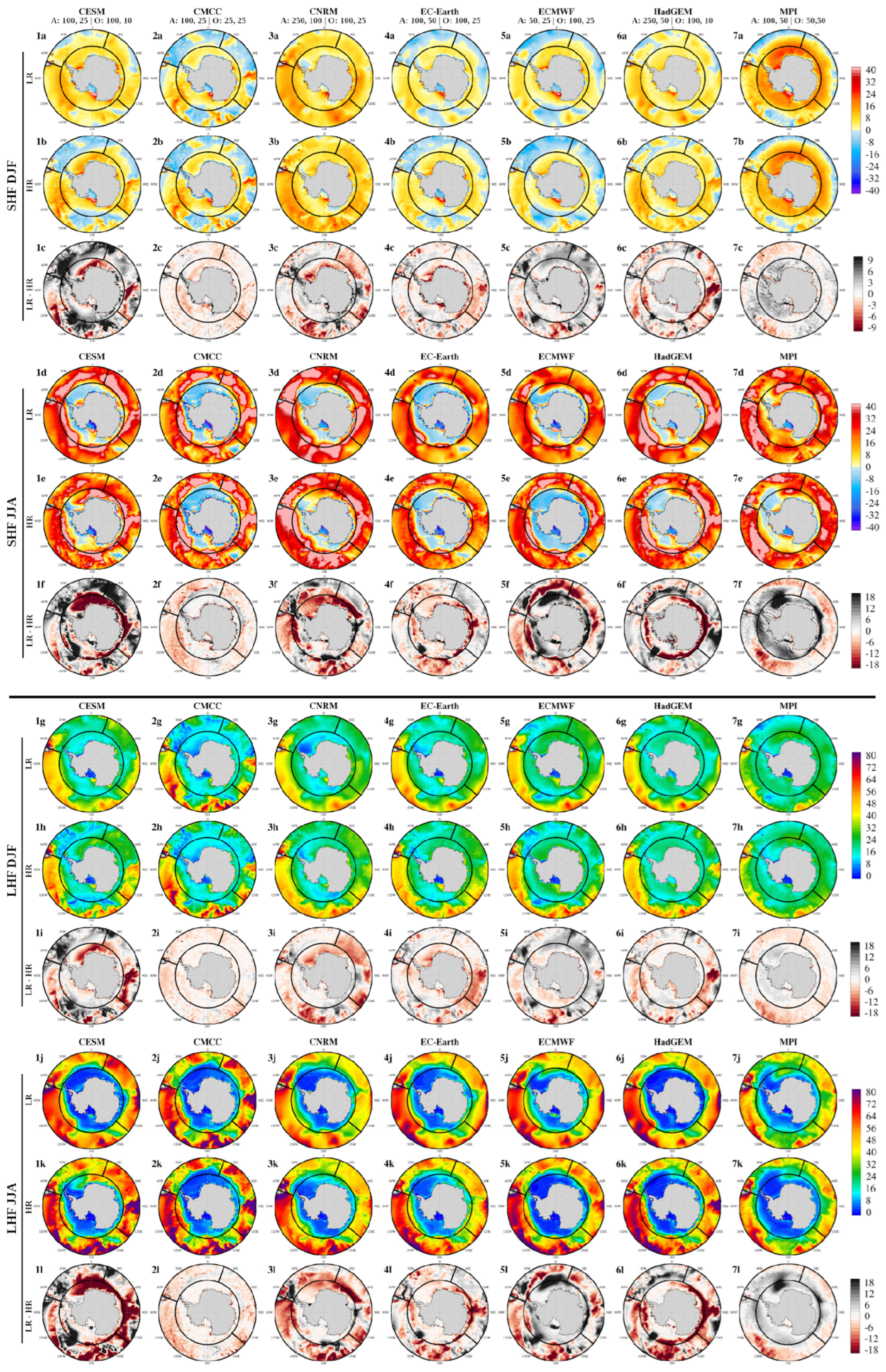
3.2. Climatological Mean State

Figure 2 shows the seasonal mean patterns of SHF and LHF from 1985 to 2014 based on MMEs and products and highlights notable spatial differences. For SHF, most products indicated heat directed out of (into) the ocean in the Indian and Pacific (Atlantic) sectors, with variations of approximately ±15 W.m−2 (Figure 2.1,5a) during summer. Among the products, the CFSR stands out as providing the most discrepant spatio-temporal patterns, displaying predominantly negative SHF values in all sectors, extending poleward up to ~70° S in summer (Figure 2.1b). SeaFlux and ERA5 exhibited some similarities in spatial pattern positioning in summer; however, ERA5 covered larger areas of ocean heat gain, while the positive values (ocean heat loss) were less intense than for SeaFlux (Figure 2.1,5a). Spatially, SHF MMEs aligned relatively well with SeaFlux (Figure 2.1d–1f), differing primarily in magnitude (Figure 2.1,2).
These summer patterns result from combined air–sea and air–sea ice interactions, including solar radiation, air-sea temperature gradients, wind forcing, and ocean circulation. According to Cai et al. [9], most of the increased ocean heat uptake observed between 50 and 65° S is primarily driven by enhanced longwave radiation (greenhouse gas emissions trapping more heat in the atmosphere), increased SHF (atmosphere warming faster than the ocean), reduced shortwave radiation (increased cloud cover due to poleward-shifting storm tracks), and decreased evaporative heat flux from the ocean (weakened easterlies and reduced shortwave radiation diminish evaporation rates). During winter, positive SHF values ranged from ~10 to 40 W.m−2 across all ocean basins in the SAZ (Figure 2.2,5a), which can be attributed to the enhanced temperature gradient between the warmer ocean surfaces and the colder MABL, leading to greater ocean heat loss compared to that observed in summer conditions [77,79,80]. In relation to other products, MMEs and SeaFlux displayed extensive areas with higher positive values (Figure 2.2a–f). For instance, the median SHF values reached 10–15 W.m−2 greater than those of other products (Figure 2.5a).
Overall, SHF was consistently lower than LHF across all datasets, typically by a factor of 3–4, consistent with Yu et al. [81]. However, some studies have reported even larger differences, reaching up to seven times or an order of magnitude [53,82], primarily driven by thermal contrast, which may enhance vertical turbulent mixing and modulate the MABL [1,80,83]. This thermal gradient also plays a crucial role in shelf water densification and atmospheric buoyancy flux patterns [84]. It is important to note that significant variations in SHF intensity and direction across datasets within each basin introduce uncertainties that can lead to misinterpretations of these processes.
LHF displayed an evident meridional gradient across the SO, with values exceeding 80 W.m−2 at lower latitudes and gradually decreasing towards the pole, reaching minima below 20 W.m−2 near the MIZ, especially during winter, when the sea ice presence inhibits air-sea heat fluxes (Figure 2.4). These results are in agreement with previous studies (e.g., [30,77]). The Pacific sector displayed the highest seasonal LHF intensity, with wintertime values peaking at ~100 W.m−2, and a significantly larger interquartile range—almost twice the amount released by the other sectors (Figure 2.3–4,5b). This asymmetry and intense ocean heat loss result from complex interrelated processes, including vertical humidity gradients [8,13,77,85] and wind-driven Ekman transport [9]. These processes are further amplified by increased surface wind stress, which strengthens the ACC and its associated mesoscale eddies. This intensification enhances air–sea heat exchange and promotes deeper convective mixing [79,86]. During winter, ocean heat exchange drives deep convective mixing, with mixed-layer depths reaching up to 700 m, resulting in significant implications for Subantarctic Mode Water (SAMW) formation and anthropogenic CO2 uptake and storage [9,10,79,86].
Figure 2. 30-year seasonal averages for SHF (1ag,2ag) and LHF (3ag,4ag). Black boxes outline the ocean sectors: Atlantic, Indian, and Pacific. Boxplots (5a–b) illustrate seasonal heat fluxes for DJF (red) and JJA (black) at a 95% confidence level. The last row shows MME LR–HR differences for SHF (1g,2g) and LHF (3g,4g).
Atmosphere 16 00402 g002
As previously discussed, the products exhibited distinct spatio-temporal patterns in SHF and LHF estimates. In both seasons, CFSR (OAFlux) consistently produced the largest SHF (LHF) discrepancies among all datasets (Figure 2). The LHF MMEs values were similar to the ERA5 and CFSR values (Figure 2.3,4) in the SAZ region, showing good agreement with ERA5 south of 63° S (Figure 2.4). In summer, compared to ERA5, the MMEs tended to overestimate SHF and underestimate LHF. In winter, this difference decreased, suggesting a better agreement between the MMEs and ERA5. Additionally, the resolution-dependent differences between MMEs (LR–HR) reached magnitudes of ±10 W.m−2, mainly in winter, with HR MMEs transferring more heat in the MIZ and higher latent heat in the Indian–Pacific sectors, whereas the LR MMEs exhibited increased sensible heat in the Atlantic–Indian sectors and the Ross Sea (Figure 2.1g–4g).
Comparing the individual HighResMIP models (Figure 3) with all products (Figure 2) revealed significant discrepancies. During summer, CMCC, EC-Earth, ECMWF model pairs, and CESM-H showed SHF spatial patterns almost similar to those of ERA5 (Figure 2.1 and Figure 3.1a–7b). In the cold season, most models agreed with the products, except for ECMWF-H and MPI-L (Figure 2.2 and Figure 3.1d–7e). For LHF, most models closely resembles ERA5 and CFSR values in both seasons (Figure 2 and Figure 3).
In the 50–63° S (south of 63° S) region, CNRM (MPI) pairs were the models that exhibited the most pronounced positive SHF values, with extensive areas of strong ocean heat loss. Our results suggest that climate models with the same ocean component can simulate different patterns of SHF ocean heat gain/loss (Figure 3). For instance, among models employing the NEMO ocean model (Table 1), CNRM and HadGEM displayed extensive areas with SHF around 40 W.m−2 in both LR and HR configurations, while CMCC, EC-Earth, and ECMWF showed large areas of heat loss (Figure 3.2a,b–6a,b). On the other hand, ECMWF and EC-Earth, which employ different versions of the same atmospheric and oceanic components (Table 1), recorded the fewest positive SHF values, particularly in the Indian and Pacific Ocean sectors (Figure 3.4a–e,5a–e). Both models follow a similar grid refinement ratio, increasing atmospheric (oceanic) resolution by a factor of 2 (4).
When evaluating the influence of grid resolution configurations based on the SHF LR–HR differences, most models displayed minor spatial variation during summer, differing mainly in magnitude (±4 W.m−2). Conversely, CESM not only recorded the highest difference values (Figure 3.1c) but also exhibited a distinct directional shift, with ocean heat uptake concentrated predominantly in the Atlantic and eastern Pacific sectors (Figure 3.1a,b). CESM remained the most prominent model in winter (Figure 3f), showing greater sensitivity to increased resolution, particularly in the Atlantic sector (±15 W.m−2), along the Antarctic coast, and in the PF and MIZ (±20 W.m−2).
The spatial distribution of LHF in summer was very similar for most models, except for the CMCC models, which displayed lower values in the Atlantic and Indian sectors and higher values in the Pacific sector (Figure 3g,h). In winter, MPI showed the lowest values across all sectors, including the Antarctic Zone (Figure 3.7g–k). Additionally, almost all HR models showed more LHF (up to 20 W.m−2) in the Drake Passage and near 60° W (Figure 3.1i,l–7i,l), emphasising the importance of eddy-resolving models in regions of high mesoscale variability. The results showed that models with increased atmospheric resolution only, such as CMCC and MPI, exhibit less sensitivity to resolution changes in simulated air–sea heat fluxes compared to models with both increased oceanic and atmospheric grid resolution. This suggests that the oceanic resolution primarily drives the low–high resolution impact [37,87], as demonstrated by the CESM model.
The CESM and HadGEM models have the most refined grids, with their oceanic components increased from 1° eddy-parameterised to 1/12° eddy-resolving, alongside atmospheric resolutions amplified by factors of 4 and 5, respectively. Furthermore, CESM also incorporates two additional vertical levels in its HR oceanic module, resulting in notable differences compared to other models. This refinement contributes to high sensitivity and variability, as well as the representation of ocean dynamics, leading to the most pronounced discrepancies in LHF and SHF values (Figure 3.1). Increased vertical and horizontal resolution improves the representation of overflows, resulting in a more realistic bathymetry that enhances the accuracy of current dynamics simulations. While mesoscale eddies can be parameterised in LR models, accurately resolving ocean currents requires significantly higher horizontal resolution [3,31,35]. HR models exhibited a noisier spatial distribution compared to their LR counterparts, reflecting the impact of increased resolution on the intrinsic variability of heat fluxes. This effect was particularly pronounced for eddy-resolving models (CESM and HadGEM), where subgrid processes are better resolved. Interestingly, despite their ability to resolve finer-scale processes, HR models exhibit lower conceptual complexity than LR models, as many physical processes represented by parameterisations in LR models become less scale-dependent in HR models [29].
Figure 3. CMIP6 HighResMIP 30-year seasonal averages for SHF (af) and LHF (gl), with their respective LR–HR differences.
Atmosphere 16 00402 g003
While high-resolution models are able to resolve finer-scale ocean dynamics, the impact of increased grid resolution varies significantly between regions and models [32,38,88]. For example, SHF and LHF values exhibited heightened sensitivity to increased atmospheric and oceanic grid resolutions in specific areas within the Atlantic (60–30° W), Indian (80–100° E), and Pacific (150° E–120° W) sectors, with differences reaching up to ±20 W.m−2. Air-sea heat gain/loss differences between LR and HR versions reached up to 30% (Figure 3c,f,i,l), emphasising significant uncertainty in their quantification within climate models. For reference, a 30% discrepancy in heat fluxes implies a similar level of uncertainty in simulated precipitation and could reflect significant disparities in the simulated hydrological cycle [79] or even inaccuracies in estimates of ocean heat content and sea level rise, primarily driven by thermal expansion and continental ice melting [89,90].
The results indicated that regions southward of 63° S are more sensitive to changes in grid resolution, with variations in air–sea heat fluxes reaching up to 50% between LR and HR values during winter, particularly in the Weddell Sea (~40° W–20° W). This region is critical for many processes, including water mass formation, global ocean circulation and turnover, and sea ice dynamics, playing a crucial role in the polar climate [9,91,92,93]. In the Weddell Sea, the representation of sea ice thickness and polynyas affects the mixed-layer depth, with convection extending into the deep ocean, which is a known issue in many Earth System Models (ESMs) and remains a significant challenge [3,68,94]. Some key physical processes, such as ice-wave interactions, floe size distribution dynamics, and small-scale heat and momentum exchanges, remain underrepresented or absent in current climate models, reinforcing the need for improved parameterisations to enhance the accuracy of polar climate simulations [4,16,45,95]. These findings highlight challenges in accurately representing complex air-sea-ice interactions in polar regions.

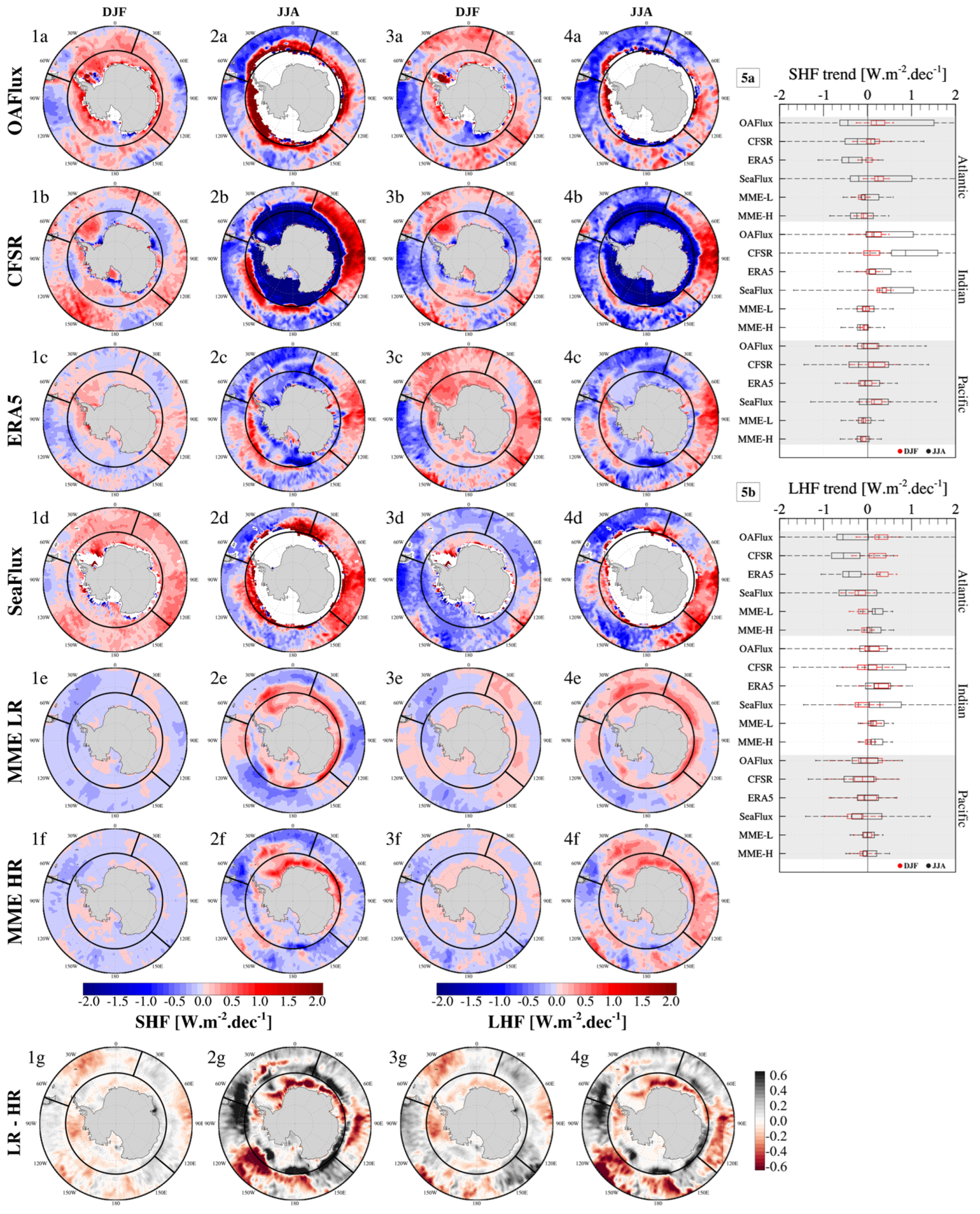
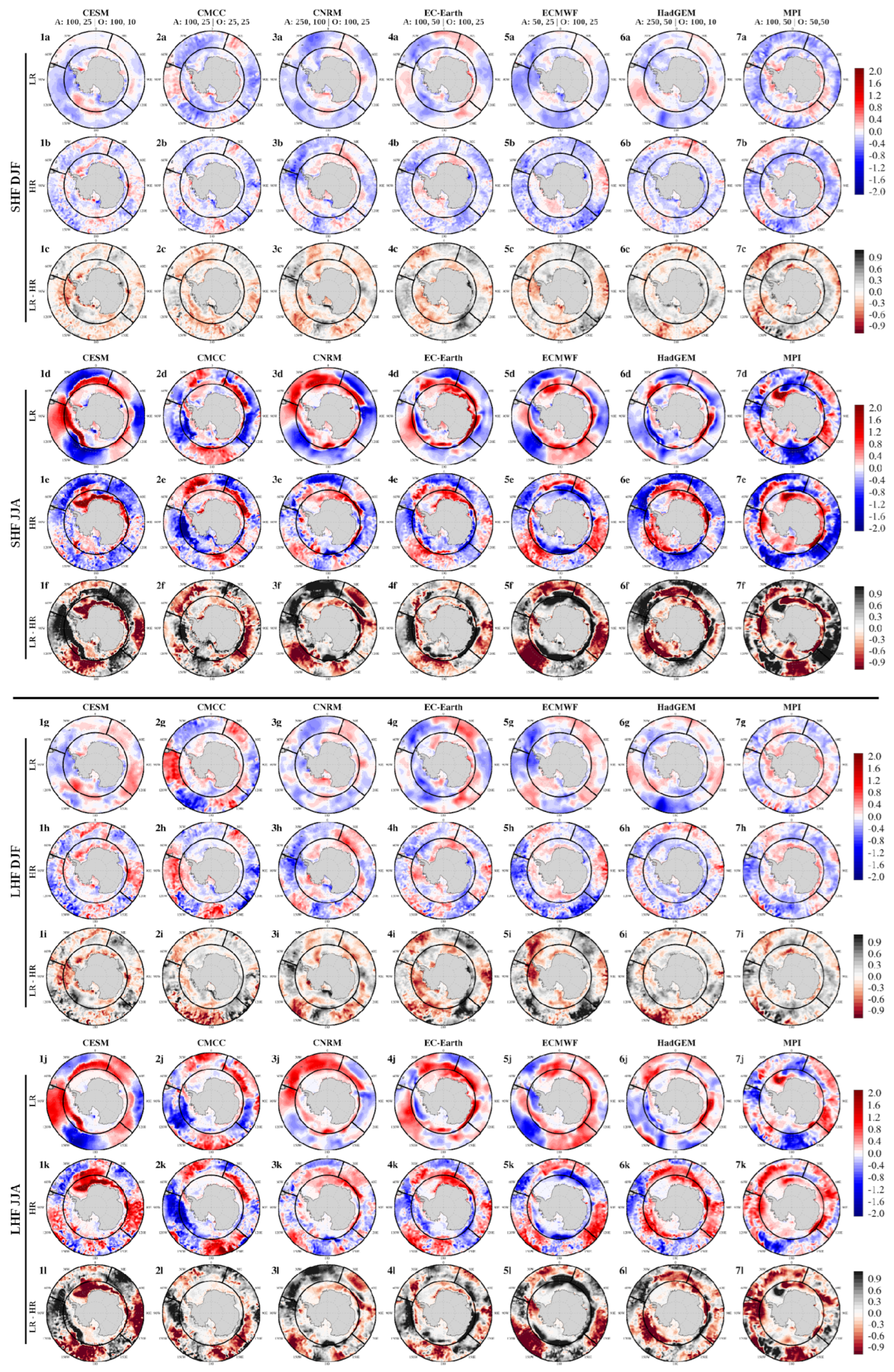
3.3. Climatological Trend

In recent decades, air-sea heat fluxes have undergone significant changes, marked by strong regional and seasonal dependencies [22,26,53,80]. In the SO, accurately representing the flux variations, particularly regional trends, remains highly uncertain, making it difficult to confidently determine long-term trends [26,31]. In this section, we evaluate these contrasting trends, showing notable variability in both magnitude and spatial distribution across different datasets. Trends in air-sea heat fluxes estimated by products and MMEs show a considerable spread among the products, which is relatively larger in winter than in summer (Figure 4). During summer, all products presented different spatial patterns, although the interquartile range of SHF trends remained positive, especially in the Atlantic and Indian sectors (Figure 4.5a). In contrast, MMEs displayed negative SHF trends, showing homogeneous spatial patterns across the ocean basins (Figure 4.1,5a). In the Antarctic Zone (south of the PF), most datasets exhibited a similar spatial pattern of accelerated positive trends (~2 W.m−2.dec−1), particularly in the Weddell Sea, albeit with smoothed values in the MMEs (±0.5 W.m−2.dec−1) (Figure 4.1).
SHF trends intensified in the cold season, with most products showing negative trends in the Atlantic sector and positive trends in the Indian sector (Figure 4.2,5b). Compared to other products, both SHF MMEs trends showed weaker magnitudes and reduced spatial variability, particularly during summer (Figure 4.1g), suggesting that MMEs may inadequately represent air-sea heat fluxes in the SO. Discrepancies among the products are not limited to SHF estimates; they also are evident in LHF estimates during both summer and winter. OAFlux and ERA5 indicated that the Atlantic Ocean loses heat at a rate of approximately 1 W.m−2.dec−1 while the eastern Pacific Ocean absorbs heat at a slightly faster rate of ~−2 W.m−2.dec−1 during summer (Figure 4.3). ERA5 showed the most extensive areas of ocean heat loss trends while SeaFlux stood out as the product with the strongest tendency for ocean heat gain across SO basins. Poleward, substantial regional differences were observed among datasets, particularly near the Antarctic coast and the sea ice edge. ERA5 showed the largest area of positive trends, while OAFlux recorded the highest positive magnitudes, particularly in the Weddell Sea (60–30° W) and parts of the Amundsen–Bellingshausen Sea (65–145° W) (Figure 4.3).
During winter, LHF trend values were more pronounced, with most products indicating a negative (positive) trend in the Atlantic (parts of the Indian) sector, except for MMEs (Figure 4.4,5b). Among them, the CFSR exhibited the strongest trends, greater than ±2 W.m−2.dec−1 in the Atlantic and Indian sectors. In the Pacific sector, there was less consensus among the datasets regarding the spatial distribution of trends, reflecting variability in regional heat flux dynamics. Although higher ocean resolution is expected to improve the estimation of air-sea heat fluxes by improving air-sea coupling and mean state representation, the inherent complexities and limited observational data can also amplify error propagation. This is evidenced by OAFlux, which, despite its lower resolution, exhibited the smallest discrepancies in SHF compared to other products during summer (Figure 4.5a). Roberts et al. [58] and Ding et al. [96] pointed out that air-sea heat fluxes are highly sensitive to horizontal resolution, particularly in regions with strong ocean fronts and mesoscale activity, where ocean dynamics significantly influence the MABL processes.
Figure 4. 30-year seasonal trends for SHF (1ag,2ag) and LHF (3ag,4ag). Black boxes outline the Atlantic, Indian, and Pacific ocean sectors. Boxplots (5ab) illustrate seasonal heat fluxes for DJF (red) and JJA (black) at a 95% confidence level. The last row shows MME LR–HR differences for SHF (1g,2g) and LHF (3g,4g).
Atmosphere 16 00402 g004
Overall, the individual model trends showed distinct characteristics (Figure 5), marked by smoother values, more pronounced spatial disparities, and divergent trend directions compared to the product-based results (Figure 4). Additionally, a notable disparity in the trend magnitudes between the products and models was also observed south of 63° S. Figure 5 shows that increasing the grid resolution of climate models enhanced spatial detail and generally amplified magnitudes, as exemplified by CESM and HadGEM (ocean grid refined from 1° to 1/12°). HR models using NEMO often calculate air-sea fluxes on the atmospheric grid and interpolate SST from the oceanic grid, as in HadGEM. This process smooths mesoscale features, introducing significant biases in air-sea feedback [32,97] and impacting long-term mean and trend patterns. To resolve mesoscale eddies, air-sea heat fluxes should ideally be computed on a finer oceanic grid, as implemented in the CESM model [98]. This approach preserves high-resolution SST anomalies, enhancing model fidelity, but also demands substantial adjustments for many coupled models and massive computing resources, significantly increasing computational costs [29,55,97].
In terms of sensitivity to refinement resolution, HR models displayed a noisier signal, indicative of ocean mesoscale activity, which was more apparent in trend patterns (Figure 5) than in the climatological mean state (Figure 3). This result suggests that higher resolution is crucial not only for accurately simulating the mean state but also for capturing dynamic variations such as trends. According to Hewitt et al. [31], the representation or parameterisation of the ocean mesoscale impacts not only the mean state of the ocean but also its variability and future climate response.
The summer LR air-sea heat flux trends were smoother compared to their HR counterparts; HR models exhibited greater spatial detail and increased values, maintaining similar overall patterns. This increase in spatial detail was even more pronounced in winter, with some models (e.g., CESM in the Pacific sector and CNRM in the Atlantic sector) showing shifts in magnitude large enough to reverse the trend direction. The models with the most significant LR–HR differences displayed a notable shift in trend signals across large areas. For example, during summer, MPI SHF showed shifts in the Atlantic sector (LR negative and HR positive trends), while for CRNM, this occurred in the Pacific sector. In winter, CESM displayed SHF trend shifts in the Indian sector, while ECMWF exhibited inverse trend signals in the Pacific with increased grid resolution. These patterns were similar for LHF trends, with the same models exhibiting shifts in corresponding sectors and seasons. Furthermore, increased LR–HR values were observed in SHF trends for EC-Earth and HadGEM (MPI) during summer (winter). Similarly, ECMWF and HadGEM (CNRM and MPI) showed amplified LHF trends during summer (winter).
Air-sea heat flux trends are more sensitive to grid refinement during winter, with SHF showing more extensive impacted areas compared to LHF. The LR–HR differences ranged from 30 to 50%, with some sectors reaching even higher values (Figure 5). This significant variation highlights the sensitivity of air-sea heat flux trends to grid refinement, demonstrating the impact of model resolution on capturing regional and seasonal changes, to represent dynamic processes (e.g., mesoscale variability) and to improve the representation of long-term trends.
Figure 5. CMIP6 HighResMIP 30-year seasonal trends for SHF (af) and LHF (gl), with their respective LR–HR differences.
Atmosphere 16 00402 g005

4. Conclusions

This study investigated the mean state and trends of SHF and LHF using four different products and seven CMIP6 HighResMIP model pairs providing air-sea heat fluxes and analysed the impact of grid resolution refinement on their estimates over the Southern Ocean. Our results revealed significant discrepancies across different datasets in both summer and winter seasons. Taylor diagrams showed that LHF trends had a more consistent seasonal performance than SHF trends, with stronger correlations and smaller deviations, indicating that SHF are more sensitive to flux estimation errors (Figure 1).
The spatial distributions of climatological mean values revealed distinct patterns in both seasons, highlighting regional variations in air-sea heat fluxes and how heat is exchanged between the ocean and atmosphere. For instance, CFSR and OAFlux displayed the largest discrepancies in SHF and LHF among all datasets studied here. When comparing both low- and high-resolution MMEs, their SHF estimates closely aligned with SeaFlux but displayed smoother magnitude variations, while LHF estimates showed good agreement with those of ERA5 and CFSR (Figure 2).
The CMIP6 HighResMIP initiative allows for comparisons between low- and high-resolution coupled models, emphasising the impact of grid refinement on simulated fluxes. Our results showed that models with finer grid refinement in oceanic and atmospheric components, such as CESM and HadGEM, have shown improved simulations of mesoscale processes, including eddy activity and boundary current dynamics. To illustrate, SHF and LHF differences between low- and high-resolution models reached up to ±20 W.m−2 in some areas, which corresponds to a spread of up to 30% in air–sea heat gain/loss (Figure 3c,f,i,l).
The discrepancies observed in the mean state were more pronounced in the trends, marked by strong regional and seasonal variations (mainly in the Pacific sector), with winter being more sensitive to resolution changes than summer (Figure 4). Most individual models displayed smoother trends compared to products, especially in regions south of 63 °S.
For the models with the finest grid refinement (CESM and HadGEM, with ocean grids refined from 1° to 1/12°), increasing the grid resolution enhanced spatial detail and generally amplified the magnitudes of air-sea heat fluxes. These differences, which can range from 30% to 50% (even higher in some sectors during winter, Figure 5), are expected to have significant impacts, including ocean mesoscale variability, sea ice dynamics, water mass formation, and global ocean circulation. These results emphasise the role of eddy-resolving models in capturing long-term climate signals and their potential impacts, as reported in previous research (e.g., [29,31,35,41]).
Over the past two decades, significant efforts have been made to estimate air-sea heat fluxes across the global ocean (e.g., [27,50,78,99,100]). Our findings highlight key discrepancies in how datasets represent ocean-atmosphere heat exchanges and the role of grid resolution in improving the representation of air-sea heat fluxes. We showed that the climatological state and long-term trends remain challenging to estimate and widely debated, particularly in data-sparse regions.
As emphasised by the Southern Ocean Observing System (SOOS) and the Southern Ocean Region Panel (SORP), improving the density and coverage of flux observations is crucial for enhancing the accuracy of heat flux estimates at regional scales [28,101]. Addressing these challenges necessitates developing advanced parameterisations for polar air-sea ice interactions, achieving the closure of global and regional heat budgets, reducing sampling uncertainties through better observational coverage, and establishing more accurate scaling parameters for surface flux estimates [4,27,29,40,53,101]. According to Souza et al. [101], these initiatives are expected to contribute to the 5th International Polar Year planned for the period from 2032 to 2033. Finally, this study reinforces the need for continued collaborative research efforts and advancements in both climate modelling techniques and observational strategies to improve our understanding and simulation of the complex dynamics driving air–sea interactions, particularly in the context of ongoing climate change.

Author Contributions

Conceptualisation, R.M. and F.C.; methodology, R.M.; software, R.M.; validation, R.M.; formal analysis, R.M. and F.C.; investigation, R.M.; resources, R.M.; data curation, R.M.; writing—original draft preparation, R.M.; writing—review and editing, R.M., F.C. and R.B.d.S.; visualisation, R.M.; supervision, R.B.d.S.; project administration, R.B.d.S.; funding acquisition, R.B.d.S. All authors have read and agreed to the published version of the manuscript.

Funding

This research was funded by the Brazilian agency CNPq for the following projects: (i) SOAC-Multiescala—Multiscale Study of the Ocean-Atmosphere-Cryosphere System (CNPq 406663/2022-0) and (ii) C3OS-Heat, Connections and Climate in the Southern Ocean (CNPq/PROANTAR 440879/2023-0). R.B.d.S. was partly funded as a CNPq Scientific Productivity Fellow (CNPq 308642/2021-0).

Institutional Review Board Statement

Not applicable.

Informed Consent Statement

Not applicable.

Data Availability Statement

The original contributions presented in the study are included in the article, and further inquiries can be directed to the corresponding author.

Acknowledgments

The authors are thankful to the Copernicus Climate Data Store (https://cds.climate.copernicus.eu, accessed on 17 September 2023), for the ERA5 ‘monthly averaged reanalysis’ dataset; the University Corporation for Atmospheric Research (UCAR) Research Data Archive for the CFSR ‘regular monthly mean product’ (https://rda.ucar.edu/datasets/d093002, accessed on 17 September 2023) and CFSv2 (https://rda.ucar.edu/datasets/d094002, accessed on 18 September 2023); the NASA Global Hydrometeorology Resource Center Distributed Active Archive Center (https://cmr.earthdata.nasa.gov, accessed on 19 September 2023) for SeaFlux ’monthly mean products’; Woods Hole Oceanographic Institution’s (WHOI) OAFlux project for monthly mean data from (https://oaflux.whoi.edu, accessed on 19 September 2023); and finally to the Earth System Grid Federation (ESGF) for CMIP6 HighRESMIP simulations (https://highresmip.org/data, accessed on 14 September 2023). The authors are also grateful to the anonymous reviewers whose comments greatly contributed to improving the manuscript.

Conflicts of Interest

The authors declare no conflicts of interest.

Abbreviations

ACCAntarctic Circumpolar Current
AZAntarctic Zone
LHFLatent Heat Flux
MABLMarine Atmospheric Boundary Layer
MIZMarginal Ice Zone
MOSTMonin–Obukhov Similarity Theory
MMEMulti-Model Ensemble
PFPolar Front
PFZPolar Frontal Zone
SAFSubantarctic Front
SAZSubantarctic Zone
SHFSensible Heat Flux
SOSouthern Ocean
STFSubtropical Front

References

  1. Tersigni, I.; Alberello, A.; Messori, G.; Vichi, M.; Onorato, M.; Toffoli, A. High-Resolution Thermal Imaging in the Antarctic Marginal Ice Zone: Skin Temperature Heterogeneity and Effects on Heat Fluxes. Earth Space Sci. 2023, 10, e2023EA003078. [Google Scholar]
  2. Yu, L. Global Air–Sea Fluxes of Heat, Fresh Water, and Momentum: Energy Budget Closure and Unanswered Questions. Annu. Rev. Mar. Sci. 2019, 11, 227–248. [Google Scholar]
  3. Beadling, R.L.; Russell, J.L.; Stouffer, R.J.; Mazloff, M.; Talley, L.D.; Goodman, P.J.; Pandde, A. Representation of Southern Ocean Properties across Coupled Model Intercomparison Project Generations: CMIP3 to CMIP6. J. Clim. 2020, 33, 6555–6581. [Google Scholar]
  4. Cronin, M.F.; Gentemann, C.L.; Edson, J.; Ueki, I.; Bourassa, M.; Brown, S.; Zhang, D. Air-Sea Fluxes with a Focus on Heat and Momentum. Front. Mar. Sci. 2019, 6, 430. [Google Scholar]
  5. Seneviratne, S.I.; Zhang, X.; Adnan, M.; Badi, W.; Dereczynski, C.; Di Luca, A.; Zhou, B. Weather and Climate Extreme Events in a Changing Climate. In Climate Change 2021: The Physical Science Basis; Contribution of Working Group I to the IPCC-AR6; Cambridge University Press: Cambridge, UK, 2021; pp. 1513–1766. [Google Scholar] [CrossRef]
  6. Zhang, R.; Dong, B.; Wen, Z.; Guo, Y.; Chen, X. Relationship between the AMOC and the Multidecadal Variability of the Midlatitude Southern Indian Ocean. J. Clim. 2023, 36, 8761–8781. [Google Scholar]
  7. Yu, L.; Zhang, Z.; Zhou, M.; Zhong, S.; Lenschow, D.H.; Li, B.; Sun, B. Trends in Latent and Sensible Heat Fluxes over the Southern Ocean. Atmos. Clim. Sci. 2012, 2, 159–173. [Google Scholar] [CrossRef]
  8. Williams, R.G.; Meijers, A.J.; Roussenov, V.M.; Katavouta, A.; Ceppi, P.; Rosser, J.P.; Salvi, P. Asymmetries in the Southern Ocean Contribution to Global Heat and Carbon Uptake. Nat. Clim. Change 2024, 14, 823–831. [Google Scholar]
  9. Cai, W.; Gao, L.; Luo, Y.; Li, X.; Zheng, X.; Zhang, X.; Xie, S.P. Southern Ocean Warming and Its Climatic Impacts. Sci. Bull. 2023, 68, 946–960. [Google Scholar]
  10. Dufour, C.O.; Frenger, I.; Frölicher, T.L.; Gray, A.R.; Griffies, S.M.; Morrison, A.K.; Schlunegger, S.A. Anthropogenic Carbon and Heat Uptake by the Ocean: Will the Southern Ocean Remain a Major Sink? US Clivar Var. 2015, 13, 1–7. [Google Scholar]
  11. Frölicher, T.L.; Sarmiento, J.L.; Paynter, D.J.; Dunne, J.P.; Krasting, J.P.; Winton, M. Dominance of the Southern Ocean in Anthropogenic Carbon and Heat Uptake in CMIP5 Models. J. Clim. 2015, 28, 862–886. [Google Scholar]
  12. Sallée, J.B.; Abrahamsen, E.P.; Allaigre, C.; Auger, M.; Ayres, H.; Zhou, S. Southern Ocean Carbon and Heat Impact on Climate. Philos. Trans. R. Soc. A 2023, 381, 20220056. [Google Scholar]
  13. Josey, S.A.; Grist, J.P.; Mecking, J.V.; Moat, B.I.; Schulz, E. A Clearer View of Southern Ocean Air–Sea Interaction Using Surface Heat Flux Asymmetry. Philos. Trans. R. Soc. A 2023, 381, 20220067. [Google Scholar] [CrossRef] [PubMed]
  14. Souza, R.B.; Pezzi, L.; Swart, S.; Oliveira, F.; Santini, M. Air–Sea Interactions over Eddies in the Brazil-Malvinas Confluence. Remote Sens. 2021, 13, 1335. [Google Scholar] [CrossRef]
  15. Chapman, C.C.; Lea, M.A.; Meyer, A.; Sallée, J.B.; Hindell, M. Defining Southern Ocean Fronts and Their Influence on Biological and Physical Processes in a Changing Climate. Nat. Clim. Change 2020, 10, 209–219. [Google Scholar] [CrossRef]
  16. Swart, S.; du Plessis, M.D.; Nicholson, S.A.; Monteiro, P.M.; Dove, L.A.; Thomalla, S.; de Souza, R.B. The Southern Ocean Mixed Layer and Its Boundary Fluxes: Fine-Scale Observational Progress and Future Research Priorities. Philos. Trans. R. Soc. A 2023, 381, 20220058. [Google Scholar] [CrossRef]
  17. Gao, Y.; Kamenkovich, I.; Perlin, N.; Kirtman, B. Oceanic advection controls mesoscale mixed layer heat budget and air–sea heat exchange in the southern ocean. J. Phys. Oceanogr. 2022, 52, 537–555. [Google Scholar] [CrossRef]
  18. Small, R.J.; Tomas, R.A.; Bryan, F.O. Storm track response to ocean fronts in a global high-resolution climate model. Clim. Dyn. 2014, 43, 805–828. [Google Scholar] [CrossRef]
  19. Chelton, D.B. Ocean-atmosphere coupling: Mesoscale eddy effects. Nat. Geosci. 2013, 6, 594–595. [Google Scholar] [CrossRef]
  20. Chelton, D.B.; Xie, S.-P. Coupled ocean-atmosphere interaction at oceanic mesoscales. Oceanography 2010, 23, 52–69. [Google Scholar] [CrossRef]
  21. Small, R.J.; de Szoeke, S.P.; Xie, S.P.; O’Neill, L.; Seo, H.; Song, Q.; Cornillon, P.; Spall, M.; Minobe, S. Air–sea interaction over ocean fronts and eddies. Dyn. Atmos. Ocean. 2008, 45, 274–319. [Google Scholar] [CrossRef]
  22. Moura, R.; de Souza, R.B.; Casagrande, F.; da Silva Lindemann, D. Air–Sea Heat Fluxes Variations in the Southern Atlantic Ocean: Present-Day and Future Climate Scenarios. Int. J. Climatol. 2024, 44, 3136–3153. [Google Scholar]
  23. Frenger, I.; Gruber, N.; Knutti, R.; Münnich, M. Imprint of Southern Ocean eddies on winds, clouds and rainfall. Nat. Geosci. 2013, 6, 608–612. [Google Scholar]
  24. O’Neill, L.W.; Chelton, D.B.; Esbensen, S.K. The effects of SST-induced surface wind speed and direction gradients on midlatitude surface vorticity and divergence. J. Clim. 2010, 23, 255–281. [Google Scholar]
  25. Swart, S.; Gille, S.T.; Delille, B.; Josey, S.; Mazloff, M.; Newman, L.; Zappa, C.J. Constraining Southern Ocean Air-Sea-Ice Fluxes through Enhanced Observations. Front. Mar. Sci. 2019, 6, 421. [Google Scholar]
  26. Sallée, J.B. Southern Ocean Warming. Oceanography 2018, 31, 52–62. [Google Scholar]
  27. Bentamy, A.; Piollé, J.F.; Grouazel, A.; Danielson, R.; Gulev, S.; Paul, F. Review and Assessment of Latent and Sensible Heat Flux Accuracy over the Global Oceans. Remote Sens. Environ. 2017, 201, 196–218. [Google Scholar] [CrossRef]
  28. Gille, S.; Josey, S.; Swart, S. New Approaches for Air-Sea Fluxes in the Southern Ocean. Eos 2016, 97. [Google Scholar]
  29. Alizadeh, O. Advances and Challenges in Climate Modeling. Clim. Change 2022, 170, 18. [Google Scholar] [CrossRef]
  30. Liu, J.; Xiao, T.; Chen, L. Intercomparisons of Air–Sea Heat Fluxes over the Southern Ocean. J. Clim. 2011, 24, 1198–1211. [Google Scholar]
  31. Hewitt, H.T.; Roberts, M.; Mathiot, P.; Biastoch, A.; Blockley, E.; Chassignet, E.P.; Zhang, Q. Resolving and Parameterizing the Ocean Mesoscale in Earth System Models. Curr. Clim. Change Rep. 2020, 6, 137–152. [Google Scholar]
  32. Roberts, M.J.; Baker, A.; Blockley, E.W.; Calvert, D.; Coward, A.; Hewitt, H.T.; Jackson, L.C.; Kuhlbrodt, T.; Mathiot, P.; Roberts, C.D.; et al. Description of the Resolution Hierarchy of the Global Coupled HadGEM3-GC3.1 Model as Used in CMIP6 HighResMIP Experiments. Geosci. Model Dev. 2019, 12, 4999–5028. [Google Scholar] [CrossRef]
  33. Haarsma, R.J.; Roberts, M.J.; Vidale, P.L.; Senior, C.A.; Bellucci, A.; Bao, Q.; von Storch, J.S. High-Resolution Model Intercomparison Project (HighResMIP v1.0) for CMIP6. Geosci. Model Dev. 2016, 9, 4185–4208. [Google Scholar] [CrossRef]
  34. Eyring, V.; Gleckler, P.J.; Heinze, C.; Stouffer, R.J.; Taylor, K.E.; Balaji, V. Towards Improved and More Routine Earth System Model Evaluation in CMIP. Earth Syst. Dyn. 2016, 7, 813–830. [Google Scholar] [CrossRef]
  35. Docquier, D.; Vannitsem, S.; Bellucci, A.; Frankignoul, C. Interactions between Ocean Heat Budget Terms in HighResMIP Climate Models Measured by the Rate of Information Transfer. EGUsphere 2022, 2022, 1–36. [Google Scholar]
  36. Moreno-Chamarro, E.; Caron, L.P.; Loosveldt Tomas, S.; Vegas-Regidor, J.; Gutjahr, O.; Moine, M.P.; Vidale, P.L. Impact of Increased Resolution on Long-Standing Biases in HighResMIP-PRIMAVERA Climate Models. Geosci. Model Dev. 2022, 15, 269–289. [Google Scholar] [CrossRef]
  37. Bellucci, A.; Athanasiadis, P.J.; Scoccimarro, E.; Ruggieri, P.; Gualdi, S.; Fedele, G.; Vidale, P.L. Air-Sea Interaction over the Gulf Stream in an Ensemble of HighResMIP Present Climate Simulations. Clim. Dyn. 2021, 56, 2093–2111. [Google Scholar] [CrossRef]
  38. Small, R.J.; Bryan, F.O.; Bishop, S.P.; Larson, S.; Tomas, R.A. What Drives Upper-Ocean Temperature Variability in Coupled Climate Models and Observations? J. Clim. 2020, 33, 577–596. [Google Scholar] [CrossRef]
  39. Hewitt, H.T.; Bell, M.J.; Chassignet, E.P.; Czaja, A.; Ferreira, D.; Griffies, S.M.; Roberts, M.J. Will High-Resolution Global Ocean Models Benefit Coupled Predictions on Short-Range to Climate Timescales? Ocean Model. 2017, 120, 120–136. [Google Scholar]
  40. Fox-Kemper, B.; Adcroft, A.; Böning, C.W.; Chassignet, E.P.; Curchitser, E.; Danabasoglu, G.; Yeager, S.G. Challenges and Prospects in Ocean Circulation Models. Front. Mar. Sci. 2019, 6, 65. [Google Scholar]
  41. Wu, P.; Roberts, M.; Martin, G.; Chen, X.; Zhou, T.; Vidale, P.L. The Impact of Horizontal Atmospheric Resolution in Modelling Air–Sea Heat Fluxes. Q. J. R. Meteorol. Soc. 2019, 145, 3271–3283. [Google Scholar] [CrossRef]
  42. Schulzweida, U. CDO User Guide (2.1.0); Zenodo; Scientific Research Publishing: Wuhan, China, 2022. [Google Scholar]
  43. Kim, Y.S.; Orsi, A.H. On the Variability of Antarctic Circumpolar Current Fronts Inferred from 1992–2011 Altimetry. J. Phys. Oceanogr. 2014, 44, 3054–3071. [Google Scholar]
  44. Orsi, A.H.; Whitworth, T., III; Nowlin, W.D., Jr. On the Meridional Extent and Fronts of the Antarctic Circumpolar Current. Deep Sea Res. Part I Oceanogr. Res. Pap. 1995, 42, 641–673. [Google Scholar]
  45. Dumont, D. Marginal Ice Zone Dynamics: History, Definitions and Research Perspectives. Philos. Trans. R. Soc. A 2022, 380, 20210253. [Google Scholar] [CrossRef] [PubMed]
  46. Vichi, M. An Indicator of Sea Ice Variability for the Antarctic Marginal Ice Zone. Cryosphere 2022, 16, 4087–4106. [Google Scholar] [CrossRef]
  47. Miaojiang, W.; Tingting, L.; Zijian, Y.; Bing, W.; Xueming, Z. Variation of Antarctic Marginal Ice Zone Extent (1989–2019). Adv. Polar Sci. 2021, 32, 341–355. [Google Scholar]
  48. Wilson, E.A.; Bonan, D.B.; Thompson, A.F.; Armstrong, N.; Riser, S.C. Mechanisms for Abrupt Summertime Circumpolar Surface Warming in the Southern Ocean. J. Clim. 2023, 36, 7025–7039. [Google Scholar]
  49. Song, X.; Yu, L. High-Latitude Contribution to Global Variability of Air–Sea Sensible Heat Flux. J. Clim. 2012, 25, 3515–3531. [Google Scholar]
  50. Gutenstein, M.; Fennig, K.; Schröder, M.; Trent, T.; Bakan, S.; Roberts, J.B.; Robertson, F.R. Intercomparison of Freshwater Fluxes over Ocean and Investigations into Water Budget Closure. Hydrol. Earth Syst. Sci. 2021, 25, 121–146. [Google Scholar]
  51. Lyu, K.; Zhang, X.; Church, J.A. Regional Dynamic Sea Level Simulated in the CMIP5 and CMIP6 Models: Mean Biases, Future Projections, and Their Linkages. J. Clim. 2020, 33, 6377–6398. [Google Scholar]
  52. Taylor, K.E. Summarizing Multiple Aspects of Model Performance in a Single Diagram. J. Geophys. Res. Atmos. 2001, 106, 7183–7192. [Google Scholar] [CrossRef]
  53. Tang, R.; Wang, Y.; Jiang, Y.; Liu, M.; Peng, Z.; Hu, Y.; Li, Z.L. A Review of Global Products of Air-Sea Turbulent Heat Flux: Accuracy, Mean, Variability, and Trend. Earth-Sci. Rev. 2024, 249, 104662. [Google Scholar] [CrossRef]
  54. Small, R.J.; Bryan, F.O.; Bishop, S.P.; Tomas, R.A. Air–Sea Turbulent Heat Fluxes in Climate Models and Observational Analyses: What Drives Their Variability? J. Clim. 2019, 32, 2397–2421. [Google Scholar] [CrossRef]
  55. Smith, S.R.; Hughes, P.J.; Bourassa, M.A. A Comparison of Nine Monthly Air–Sea Flux Products. Int. J. Climatol. 2011, 31, 1002–1027. [Google Scholar] [CrossRef]
  56. Srivastava, P.; Sharan, M. Analysis of dual nature of heat flux predicted by Monin-Obukhov similarity theory: An impact of empirical forms of stability correction functions. J. Geophys. Res. Atmos. 2019, 124, 3627–3646. [Google Scholar] [CrossRef]
  57. Beljaars, A.; Dutra, E.; Balsamo, G.; Lemarié, F. On the numerical stability of surface–atmosphere coupling in weather and climate models. Geosci. Model Dev. 2017, 10, 977–989. [Google Scholar] [CrossRef]
  58. Roberts, M.J.; Hewitt, H.T.; Hyder, P.; Ferreira, D.; Josey, S.A.; Mizielinski, M.; Shelly, A. Impact of Ocean Resolution on Coupled Air-Sea Fluxes and Large-Scale Climate. Geophys. Res. Lett. 2016, 43, 10430. [Google Scholar] [CrossRef]
  59. Chang, P.; Zhang, S.; Danabasoglu, G.; Yeager, S.G.; Fu, H.; Wang, H.; Wu, L. An Unprecedented Set of High-Resolution Earth System Simulations for Understanding Multiscale Interactions in Climate Variability and Change. J. Adv. Model. Earth Syst. 2020, 12, e2020MS002298. [Google Scholar] [CrossRef]
  60. Scoccimarro, E.; Peano, D.; Gualdi, S.; Bellucci, A.; Lovato, T.; Fogli, P.G.; Navarra, A. Extreme Events Representation in CMCC-CM2 High and Very-High-Resolution General Circulation Models. Geosci. Model Dev. Discuss. 2021, 15, 1841–1854. [Google Scholar] [CrossRef]
  61. Voldoire, A.; Saint-Martin, D.; Sénési, S.; Decharme, B.; Alias, A.; Chevallier, M.; Waldman, R. Evaluation of CMIP6 Deck Experiments with CNRM-CM6-1. J. Adv. Model. Earth Syst. 2019, 11, 2177–2213. [Google Scholar] [CrossRef]
  62. Haarsma, R.; Acosta, M.; Bakhshi, R.; Bretonnière, P.A.B.; Caron, L.P.; Castrillo, M.; Wyser, K. HighResMIP Versions of EC-Earth: EC-Earth3P and EC-Earth3P-HR. Description, Model Performance, Data Handling and Validation. Geosci. Model Dev. Discuss. 2020, 13, 3507–3527. [Google Scholar] [CrossRef]
  63. Roberts, C.D.; Senan, R.; Molteni, F.; Boussetta, S.; Mayer, M.; Keeley, S.P. Climate Model Configurations of the ECMWF Integrated Forecasting System (ECMWF-IFS Cycle 43r1) for HighResMIP. Geosci. Model Dev. 2018, 11, 3681–3712. [Google Scholar]
  64. Gutjahr, O.; Putrasahan, D.; Lohmann, K.; Jungclaus, J.H.; von Storch, J.S.; Brüggemann, N.; Stössel, A. Max Planck Institute Earth System Model (MPI-ESM1.2) for the High-Resolution Model Intercomparison Project (HighResMIP). Geosci. Model Dev. 2019, 12, 3241–3281. [Google Scholar]
  65. Bell, B.; Hersbach, H.; Simmons, A.; Berrisford, P.; Dahlgren, P.; Horányi, A.; Thépaut, J.N. The ERA5 Global Reanalysis: Preliminary Extension to 1950. Q. J. R. Meteorol. Soc. 2021, 147, 4186–4227. [Google Scholar]
  66. Hersbach, H.; Bell, B.; Berrisford, P.; Biavati, G.; Horányi, A.; Muñoz Sabater, J.; Nicolas, J.; Peubey, C.; Radu, R.; Rozum, I.; et al. ERA5 Monthly Averaged Data on Single Levels from 1979 to Present. Copernic. Clim. Chang. Serv. (C3S) Clim. Data Store (CDS) 2019, 10, 252–266. [Google Scholar]
  67. Kennedy, J.; Reyner, N.; Millington, S.C.; Saunby, M. The Met Office Hadley Centre Sea Ice and Sea-Surface Temperature Data Set, Version 2, Part 2: Sea Surface Temperature Analysis. Met Off. Hadley Cent. 2016, 119, 2864–2889. [Google Scholar]
  68. Titchner, H.A.; Rayner, N.A. The Met Office Hadley Centre Sea Ice and Sea Surface Temperature Data Set, Version 2: 1. Sea Ice Concentrations. J. Geophys. Res. Atmos. 2014, 119, 2864–2889. [Google Scholar]
  69. Saha, S.; Moorthi, S.; Pan, H.L.; Wu, X.; Wang, J.; Nadiga, S.; Goldberg, M. NCEP Climate Forecast System Reanalysis (CFSR) Monthly Products, January 1979 to December 2010. J. Clim. 2010, 23, 3482–3505. [Google Scholar]
  70. Saha, S.; Moorthi, S.; Wu, X.; Wang, J.; Nadiga, S.; Tripp, P.; Becker, E. The NCEP Climate Forecast System Version 2. J. Clim. 2014, 27, 2185–2208. [Google Scholar]
  71. Fairall, C.W.; Bradley, E.F.; Hare, J.E.; Grachev, A.A.; Edson, J.B. Bulk Parameterization of Air–Sea Fluxes: Updates and Verification for the COARE Algorithm. J. Clim. 2003, 16, 571–591. [Google Scholar]
  72. Webster, P.J.; Lukas, R. TOGA COARE: The Coupled Ocean–Atmosphere Response Experiment. Bull. Am. Meteorol. Soc. 1992, 73, 1377–1416. [Google Scholar]
  73. Liu, W.T.; Katsaros, K.B.; Businger, J.A. Bulk Parameterization of Air-Sea Exchanges of Heat and Water Vapor Including the Molecular Constraints at the Interface. J. Atmos. Sci. 1979, 36, 1722–1735. [Google Scholar]
  74. Edson, J.B.; Jampana, V.; Weller, R.A.; Bigorre, S.P.; Plueddemann, A.J.; Fairall, C.W.; Hersbach, H. On the Exchange of Momentum over the Open Ocean. J. Phys. Oceanogr. 2013, 43, 1589–1610. [Google Scholar]
  75. Roberts, J.B.; Clayson, C.A.; Robertson, F.R. SeaFlux v3: An Updated Climate Data Record of Ocean Turbulent Fluxes. 2020. [Google Scholar]
  76. Yu, L.; Jin, X.; Weller, R.A. Multidecade Global Flux Datasets from the Objectively Analyzed Air-Sea Fluxes Project: Latent and Sensible Heat Fluxes, Ocean Evaporation, and Related Surface Meteorological Variables; OAFlux Project Technical Report OA-2008-01; Woods Hole Oceanographic Institution: Woods Hole, MA, USA, 2008; p. 64. [Google Scholar]
  77. Song, X. Explaining the Zonal Asymmetry in the Air-Sea Net Heat Flux Climatology over the Antarctic Circumpolar Current. J. Geophys. Res. Oceans 2020, 125, e2020JC016215. [Google Scholar]
  78. Chou, S.H.; Nelkin, E.; Ardizzone, J.; Atlas, R.M. A Comparison of Latent Heat Fluxes over Global Oceans for Four Flux Products. J. Clim. 2004, 17, 3973–3989. [Google Scholar]
  79. Tamsitt, V.; Cerovečki, I.; Josey, S.A.; Gille, S.T.; Schulz, E. Mooring Observations of Air–Sea Heat Fluxes in Two Subantarctic Mode Water Formation Regions. J. Clim. 2020, 33, 2757–2777. [Google Scholar]
  80. Herman, A. Trends and Variability of the Atmosphere–Ocean Turbulent Heat Flux in the Extratropical Southern Hemisphere. Sci. Rep. 2015, 5, 14900. [Google Scholar]
  81. Yu, L.; Zhang, Z.; Zhong, S.; Zhou, M.; Gao, Z.; Wu, H.; Sun, B. An Inter-Comparison of Six Latent and Sensible Heat Flux Products over the Southern Ocean. Polar Res. 2011, 30, 10167. [Google Scholar]
  82. Yu, L.; Weller, R.A. Objectively Analyzed Air–Sea Heat Fluxes for the Global Ice-Free Oceans (1981–2005). Bull. Am. Meteorol. Soc. 2007, 88, 527–540. [Google Scholar] [CrossRef]
  83. Yu, L.; Jin, X.; Josey, S.A.; Lee, T.; Kumar, A.; Wen, C.; Xue, Y. The Global Ocean Water Cycle in Atmospheric Reanalysis, Satellite, and Ocean Salinity. J. Clim. 2017, 30, 3829–3852. [Google Scholar]
  84. Meredith, M.P.; Brandon, M.A. Oceanography and Sea Ice in the Southern Ocean. In Sea Ice; Wiley Online Library: Hoboken, NJ, USA, 2017; pp. 216–238. [Google Scholar]
  85. Hague, M.; Münnich, M.; Gruber, N. Zonally Asymmetric Increase in Southern Ocean Heat Content. J. Clim. 2024, 37, 6585–6604. [Google Scholar]
  86. Du Plessis, M.D.; Swart, S.; Biddle, L.C.; Giddy, I.S.; Monteiro, P.M.; Reason, C.J.C.; Nicholson, S.A. The Daily-Resolved Southern Ocean Mixed Layer: Regional Contrasts Assessed Using Glider Observations. J. Geophys. Res. Oceans. 2022, 127, e2021JC017760. [Google Scholar] [CrossRef]
  87. Tsartsali, E.E.; Haarsma, R.J.; Athanasiadis, P.J.; Bellucci, A.; de Vries, H.; Drijfhout, S.; Roberts, C.D. Impact of Resolution on the Atmosphere–Ocean Coupling along the Gulf Stream in Global High-Resolution Models. Clim. Dyn. 2022, 58, 3317–3333. [Google Scholar] [CrossRef]
  88. Selivanova, J.; Iovino, D.; Cocetta, F. Past and Future of the Arctic Sea Ice in High-Resolution Model Intercomparison Project (HighResMIP) Climate Models. Cryosphere 2024, 18, 2739–2763. [Google Scholar] [CrossRef]
  89. Wild, M. The Global Energy Balance as Represented in CMIP6 Climate Models. Clim. Dyn. 2020, 55, 553–577. [Google Scholar] [CrossRef] [PubMed]
  90. Cheng, L.; Abraham, J.; Trenberth, K.E.; Fasullo, J.; Boyer, T.; Locarnini, R.; Zhu, J. Upper Ocean Temperatures Hit Record High in 2020. Adv. Atmos. Sci. 2021, 38, 523–530. [Google Scholar] [CrossRef]
  91. Rintoul, S.R. The Global Influence of Localized Dynamics in the Southern Ocean. Nature 2018, 558, 209–218. [Google Scholar] [CrossRef]
  92. Liu, W.; Lu, J.; Xie, S.P.; Fedorov, A. Southern Ocean Heat Uptake, Redistribution, and Storage in a Warming Climate: The Role of Meridional Overturning Circulation. J. Clim. 2018, 31, 4727–4743. [Google Scholar]
  93. Meredith, M.P. The Global Importance of the Southern Ocean and the Key Role of Its Freshwater Cycle. Ocean Chall. 2019, 23, 27–32. [Google Scholar]
  94. Mohrmann, M.; Heuzé, C.; Swart, S. Southern Ocean Polynyas in CMIP6 Models. Cryosphere 2021, 15, 4281–4313. [Google Scholar] [CrossRef]
  95. Casagrande, F.; Stachelski, L.; de Souza, R.B. Assessment of Antarctic Sea Ice Area and Concentration in Coupled Model Intercomparison Project Phase 5 and Phase 6 Models. Int. J. Climatol. 2023, 43, 1314–1332. [Google Scholar] [CrossRef]
  96. Ding, T.; Zhou, T.; Chen, X.; Zou, L.; Li, P.; Roberts, M.J.; Wu, P. Enhanced Turbulent Heat Fluxes Improve Meiyu-Baiu Simulation in High-Resolution Atmospheric Models. J. Adv. Model. Earth Syst. 2021, 13, e2020MS002430. [Google Scholar]
  97. Moreton, S.; Ferreira, D.; Roberts, M.; Hewitt, H. Air-Sea Turbulent Heat Flux Feedback over Mesoscale Eddies. Geophys. Res. Lett. 2021, 48, e2021GL095407. [Google Scholar]
  98. Yang, P.; Jing, Z.; Wu, L. An Assessment of Representation of Oceanic Mesoscale Eddy-Atmosphere Interaction in the Current Generation of General Circulation Models and Reanalyses. Geophys. Res. Lett. 2018, 45, 11856–11865. [Google Scholar]
  99. Loeb, N.G.; Mayer, M.; Kato, S.; Fasullo, J.T.; Zuo, H.; Senan, R.; Balmaseda, M. Evaluating Twenty-Year Trends in Earth’s Energy Flows from Observations and Reanalyses. J. Geophys. Res. Atmos. 2022, 127, e2022JD036686. [Google Scholar]
  100. Gentemann, C.L.; Clayson, C.A.; Brown, S.; Lee, T.; Parfitt, R.; Farrar, J.T.; Zlotnicki, V. FluxSat: Measuring the Ocean–Atmosphere Turbulent Exchange of Heat and Moisture from Space. Remote Sens. 2020, 12, 1796. [Google Scholar] [CrossRef]
  101. de Souza, R.B.; Dufour, C.O.; Haumann, A.; Martin, T.; Pezzi, L.P.; Robinson, N.; Scardilli, A. Editorial: Highlighting Ocean Research, Data and Networks of Antarctic Programs. Exchanges 2024, 1, 1–48. [Google Scholar]
Disclaimer/Publisher’s Note: The statements, opinions and data contained in all publications are solely those of the individual author(s) and contributor(s) and not of MDPI and/or the editor(s). MDPI and/or the editor(s) disclaim responsibility for any injury to people or property resulting from any ideas, methods, instructions or products referred to in the content.

