Abstract
Understanding the characteristics of wildfires in the Beijing–Tianjin–Hebei (BTH) region is crucial for improving the monitoring of local wildfire danger. Our investigation first establishes the spatial distributions of fire weather index (FWI) distributions and satellite-observed wildfire occurrences. The FWI provides a reasonably accurate representation of wildfire danger in the BTH region. Through Self-Organizing Maps (SOM) clustering analysis, we identify nine distinct spatial patterns in FWI composites. Notably, the annual frequency of SOM modes 2 and 7 has shown a significant increasing trend over the past 40 years. The spatial distribution of the highest FWI values in these two modes is in the southern and central BTH regions, respectively. Subsequently, we examine the relationship between FWI variations and atmospheric circulation patterns. A synoptic analysis indicates that the increased fuel availability index observed in SOM modes 2 and 7 can be primarily attributed to two key factors. One is a post-trough system, which is marked by a decrease in water vapor transport. The other is a high-pressure system, which is associated with higher temperatures and drought conditions. Finally, the relative contributions of the fuel available index and the wildfire spread rate index to the FWI are quantified using a partial differential approach. The variations in the fuel available index are the primary drivers of the high FWI values in these two SOM patterns. This study underscores the importance of analyzing the synergistic effects of multiple atmospheric circulation patterns on the fuel availability index, which is critical for improving wildfire danger prediction at different timescales in the BTH region.
1. Introduction
Wildfires, as a significant natural disturbance in global ecosystems, have garnered increasing attention in recent years [1,2]. As reported by the Chinese Academy of Sciences (2023) [3], the global burned area has reached 1.03 million km2 over the past 20 years, highlighting the destructive impact of wildfires on ecosystems and their adverse effects on human health and socioeconomic development [4,5]. Wildfires alter global carbon storage by destroying surface vegetation, releasing greenhouse gases, modifying soil properties, and affecting the carbon cycle, thereby having profound implications for the global earth system [6]. Therefore, wildfires, as an important driver of global change, have attracted widespread attention.
Over the past several decades, global warming has led to a significantly increasing frequency of extreme climate events, thereby increasing the frequency and intensity of wildfires [7,8]. Both observation data and climate model results have demonstrated that extreme high temperatures and drought accelerate the moisture evaporation from vegetation and soil, resulting in drier conditions in forests and grasslands, thereby increasing wildfire risks [9,10]. For instance, rising temperatures and reduced precipitation in the western United States have significantly increased the likelihood of extreme climate events, leading to more frequent and larger wildfires in the region [11,12]. These changes have also caused an unprecedented increase in both the intensity and spatial extent of wildfires in California, with some fires reaching historically large scales [13]. Similarly, China has experienced 130,000 forest fires over the past two decades, covering a total area of 3.86 million hectares, approximately 6% of the global total [3]. Among these, the forest fire dangers in North and Southwest China are particularly significant [14,15]. Overall, the impact of climate change on forest fire risk is increasing. Wildfire dangers are likely to rise further, particularly in climate-sensitive regions, such as Northern China. Therefore, adapting to climate change and strengthening wildfire prevention and control measures are critical tasks in global climate change mitigation.
The Beijing–Tianjin–Hebei (BTH) region is located in the Eastern Asian monsoon zone [16,17] and is recognized as a typical climate-sensitive area [18,19]. Surrounded by the Taihang Mountains in the west and the Yanshan Mountains in the north, the BTH region is primarily covered by forests and grasslands. As global warming has intensified, the ecosystems in the BTH region have shown more pronounced changes [20]. The high temperatures and drought conditions in the spring and summer have led to the drying of soils and vegetation, thereby increasing the probability of wildfires [21,22]. According to the Beijing Emergency Management Bureau, between 2016 and 2019, a total of 43 fires occurred in the areas surrounding Beijing due to climatic conditions, resulting in significant impacts. Therefore, wildfire risk in the BTH region has become a critical challenge under climate change and demands immediate mitigation strategies.
The fire weather index (FWI) model is an important tool for assessing wildfire danger, with significant advantages in fire prediction and management. The FWI is calculated based on the moisture balance theory with a time lag [23,24]. This approach comprehensively integrates multiple meteorological factors and quantifies their combined influence on wildfire occurrence through a weighted calculation. The advantage of FWI is not only its ability to assess fire danger levels but also to reflect the impact of climate change. By incorporating FWI, government officials could more accurately assess fire danger, optimize resource allocation, and enhance the efficiency of disaster prevention and mitigation efforts. As a result, this model has been widely applied in wildfire warning systems in the BTH region, as well as in studies on the impact of climate change on wildfire risk [15,25,26], which could demonstrate its significant application and scientific research value.
This study aims to explore the contribution of climate change to the FWI in the BTH region. We addressed the following questions: (1) What are the spatial patterns of the FWI in the BTH region using self-organizing maps? (2) What are the dominant factors influencing FWI variations? (3) What are the differences in spatial patterns for FWI between historical periods and Shared Socioeconomic Pathway scenarios (SSPs)? The remainder of this paper is structured as follows: Section 2 outlines the materials and methods, Section 3 presents the results, Section 4 discusses the findings, and Section 5 concludes the study.
2. Materials and Methods
2.1. Data
The datasets utilized in this study include the ERA5 dataset from the European Centre for Medium-Range Weather Forecasts (ECMWF), the Global Fire Emissions Database version 4.1 (GFED v4.1), and simulation outputs from the Coupled Model Intercomparison Project Phase 6 (CMIP6).
The ERA5 global reanalysis meteorological data were produced by the fifth generation of the ECMWF reanalysis system. ERA5 provided higher spatial (0.25° × 0.25°) and temporal (hourly) resolutions, as well as a greater number of pressure levels (137 levels) compared to previous reanalysis products [27,28,29]. Numerous studies have shown that ERA5 outperforms other surface weather reanalysis methods [30,31]. For this study, we utilized ERA5 hourly data from 1981 to 2020, which include maximum surface air temperature (Tmax), precipitation, relative humidity (RH), wind speed (WS), geopotential height at 500 hPa and 850 hPa pressure levels, and sea level pressure.
The GFED v4.1 dataset provides biomass-burning emissions derived using a top-down calculation methodology [32]. It offers daily emission estimates at a spatial resolution of 0.25° × 0.25° for the period of 1997–2020. The dataset includes key variables such as the burned area, dry matter mass, etc. GFED v4.1 represented a significant improvement over its predecessor, GFED v3, primarily due to the incorporation of emissions from small fires [33,34].
The daily simulation data used in this study, including Tmax, precipitation, RH, and WS, were obtained from 16 global climate models (Table 1) through the CMIP6. Four experimental setups were utilized, including historical simulations and projections based on three SSPs: SSP126, SSP245, and SSP585. The historical simulations incorporated real-time, dynamic external forcings, such as greenhouse gas concentrations and land use/land cover changes. The SSP126, SSP245, and SSP585 scenarios represent different future pathways of societal development and greenhouse gas emissions.

Table 1.
The information on CMIP6 models.
Provincial boundary data were obtained from the Resource and Environment Science and Data Center, Chinese Academy of Sciences (RESDC-CAS, https://www.resdc.cn/, accessed on 20 July 2023). The map data were obtained through satellite remote sensing, aerial photography, and field surveys. Subsequently, the data underwent preprocessing procedures, such as data cleaning, format conversion, and coordinate correction, to ensure their accuracy and consistency.
2.2. Methods
2.2.1. Fire Weather Index Model
The FWI model is based on the time-lag equilibrium moisture content theory, which effectively links meteorological conditions to fuel moisture content. The FWI model consists of six components: the Initial Spread Index (ISI), the Duff Moisture Code (DMC), the Drought Code (DC), the Fine Fuel Moisture Code (FFMC), the Build-Up Index (BUI), and the FWI itself, which could be calculated using daily meteorological observations, including Tmax, RH, WS, and precipitation. The FWI integrates the BUI, which represents the available fuel index calculated from Tmax, RH, and precipitation, and the ISI, which represents the wildfire spread rate index calculated from WS [23,35]. Notably, the FWI is commonly used as an indicator of whether local meteorological conditions are conducive to wildfire occurrence. It has been proven to have strong positive correlations with the burned area across much of the global burnable land mass [36,37]. The FWI can be calculated as follows:
(a) FFMC. The fine fuel moisture code reflects the changes in the moisture content of fine combustible material and surface dead leaves in forests.
(b) DMC. The DMC reflects the moisture content in the lower combustible layer of semi-decomposed, relatively loose deadfall.
where m is the moisture content of the fine combustible materials, which can be obtained by Equations (2) and (3).
(c) DC. The drought code reflects the moisture content of the deep combustible layer at 10–20 cm in the soil layer, which generally varies seasonally.
where pr is the daily precipitation (mm).
(d) ISI. The ISI reflects the rate at which a forest fire spreads when there is a constant amount of combustible material. The ISI can be calculated by integrating the fine combustible material moisture content and wind speed.
where f(W) is the wind speed function in the ISI.
(e) BUI. The BUI represents how well-combustible materials affect fire spread and can calculated by combining the DMC and the DC.
(f) FWI. The FWI encompasses the abovementioned processes and is regarded as the final output of the FWI system. Generally, it reflects the intensity of fire danger.
where BUI indicates the fuel available index calculated by Tmax, RH, and precipitation. ISI indicates the wildfire spread rate index calculated by WS.
2.2.2. Self-Organizing Map Analysis
The Self-Organizing Map (SOM) is a neural network-based clustering technique that has recently gained application in earth sciences for characterizing continuous spatial patterns [38,39]. SOM analysis of wildfire patterns is analogous to traditional principal component analysis, where the nodes of the Self-Organizing Map correspond to the principal modes of the underlying wildfire data. In this study, we first used the SOM algorithm to assign daily FWI values to spatial patterns of a preset number. We established 9 spatial patterns in this study. Then, the SOM algorithm generated spatial patterns that maximize their similarity to the underlying wildfire fields by minimizing the Euclidian distance and assigning each daily wildfire field to the best matching pattern. The SOM patterns approximately represent a composite of relatively comparable wildfire fields because they are approximately the mean of the allocated wildfire fields. Thus, these complete processes allow the visualization of a reduced space continuum of spatial patterns in the daily wildfire dataset.
2.2.3. Derivation of Partial Differential Equations for Fire Weather Index
Following Section 2.2.1, the FWI index directly combines BUI and ISI. To derive the partial differential equation of FWI, we simplify the equations for the FWI. The specific processes are shown as follows.
First step:
Based on Equation (2), we find that f(D) is a function of BUI. So, we substitute the calculated BUI with Equation (2) to obtain f(D) and regard f(D) as the new BUI to simplify the equation. The simplified equation is defined as Equation (15).
Second step:
Similarly, we also consider that ln(FWI(t)), ln(ISI(t)), and ln(BUI(t)) are functions of FWI(t), ISI(t), and BUI(t), respectively. So, we calculate the logarithm results of FWI(t), ISI(t), and BUI(t) as new FWI(t), ISI(t), and BUI(t). The simplified equation is further defined as Equation (16).
Third step:
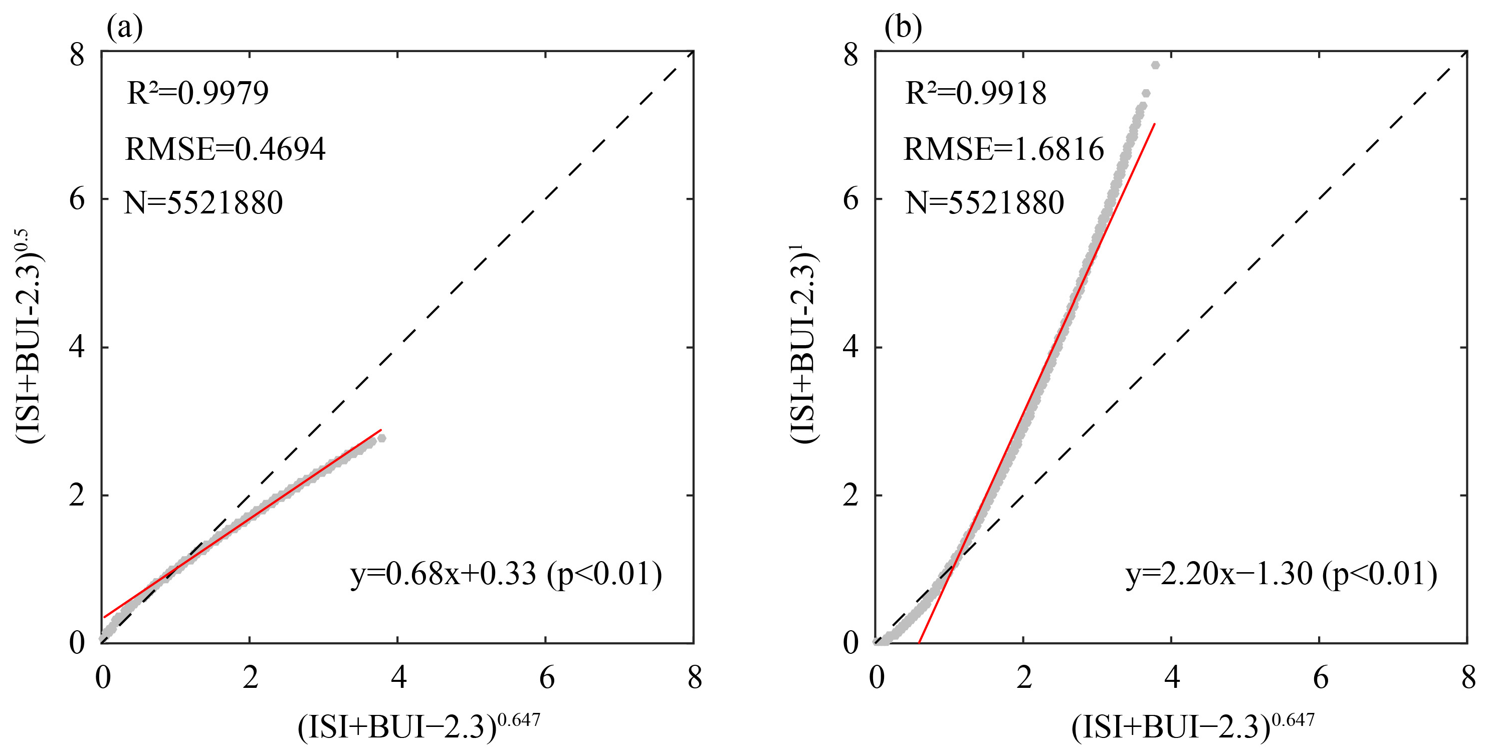
We attempted to derive the partial differential equation of Equation (16), from which we quantified the effect of BUI and ISI on FWI. However, the power index of (ISI(t) + BUI(t) − 2.3) is 0.64, which cannot be expanded to calculate the partial derivative. So, we used the calculated BUI and ISI results to calculate (ISI + BUI − 2.3)0.647, (ISI + BUI − 2.3)0.5, and (ISI + BUI − 2.3)1 for all grid cells in the BTH region and compared the differences among them (Figure 1). We found that the range of (ISI + BUI − 2.3)0.647 is from 0 to 4. The range of (ISI + BUI − 2.3)0.5 is 0 to 3, while the range of (ISI + BUI − 2.3)1 is 0 to 8. The result of (ISI + BUI − 2.3)0.5 is closer to the result with (ISI + BUI − 2.3)0.647. The correlation coefficient and RMSE between (ISI + BUI − 2.3)0.647 and (ISI + BUI − 2.3)0.5 are 0.9979 and 0.4694, respectively. The correlation coefficient and RMSE between (ISI + BUI − 2.3)0.647 and (ISI + BUI − 2.3)1 is 0.9918 and 1.6816, respectively. Although the correlation coefficients of the two groups are close, the difference between the RMSEs is significant. We consider that the power function of 0.647 can be replaced by that of 0.5 to be used in the derivation of partial differential equations. Notably, Δ is the difference between (ISI + BUI − 2.3)0.647 and (ISI + BUI − 2.3)0.5. In this study, the purpose of calculating the partial differential equation for this equation is to quantify the contribution of ISI and BUI to the FWI using a difference-based approach. To achieve this target, using 0.5 as the exponent for partial differentiation also offers the following three advantages: (a) mathematical simplification—when the exponent is 0.5, the difference approximation error is smaller because the difference method is essentially a linear approximation, and the square root function has lower curvature (with a smaller second derivative), making it closer to linear within a local interval; (b) strong numerical stability—when ISI + BUI − 2.3 approaches 0, the power function with an exponent of 0.647 amplifies the rate at which the denominator approaches zero, potentially causing numerical instability, and by changing the exponent to 0.5, the square root function slows down the growth of the denominator, significantly improving the robustness of the computation; (c) explanatory optimization of models—the square root function has lower sensitivity to the input, and the decay rate of the contribution of ISI and BUI decreases more slowly as their values increase, making the results easier to interpret.
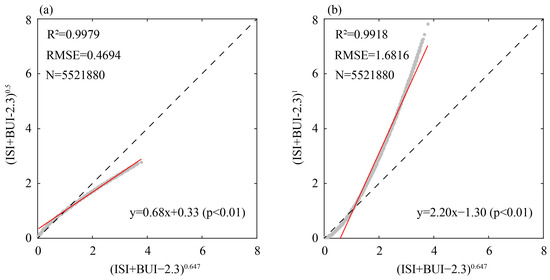
Figure 1.
Scatterplot of a power function with (ISI + BUI − 2.3)x (power exponent of 0.5 (a) and 1 (b)) as base (N is sample number; the red lines represent the trend).
Fourth step:
Based on the principle of the chain rule, which states that for y = f(g(t)), the derivative is given by dy/dt = f′(g(t)) × g′(t), we apply the chain rule to both sides of Equation (17) to obtain the partial derivative with respect to t. This ultimately results in the partial differential equation shown in Equations (18) and (19).
where is the FWI variation in SOM modes. is the fuel-available index variation in SOM modes. is the wildfire spread rate index variation in SOM modes. and is the result of the wildfire spread rate index climatology. and is the result of the fuel available index climatology. The term of δ is the constant term, which represents the residual. Let and , and Equation (6) can be converted into the following form.
2.2.4. Contributions of the Fuel Available Index and Wildfire Spread Rate Index on the Fire Weather Index
Following Equation (19), we can obtain the variations in the FWI, BUI, and ISI. Then, we can calculate to represent the contribution of the fuel available index to the FWI. Similarly, represents the contribution of the wildfire spread rate index to the FWI. Notably, the sum of the contributions of the variations in the fuel available index and the wildfire spread rate index is not equal to 100%. The reason is that we conduct simplification and an approximate transformation when calculating the partial differential equations, as shown in Figure 1. Although the results still exhibit differences, the relative contributions are within acceptable limits.
3. Results
3.1. Spatial Characteristics of the Fire Weather Index and Wildfire Days
The BTH region has experienced significant climate variability and extreme climate events (e.g., heatwaves and droughts) in the context of global warming, which amplifies wildfire risks. Here, we quantified the frequency of wildfires by counting the wildfire days and compared them with the FWI to reveal how the FWI responded to wildfire frequency. Compared to other months, the FWI values are significantly higher from April to May throughout the BTH region, indicating a higher probability of wildfire danger during this period. Based on peak FWI values, we defined April−May as the wildfire season most affected by climatic conditions.
Figure 2 shows the multi-year means and trends in the April−May FWI-based and GFED-based wildfire days within the BTH region. We found that the spatial pattern of the multi-year mean FWI is characterized by a decreasing-then-increasing gradient along the northwest-southeast transect. The highest FWI values (>40) are clustered in the northwest, while central and southern subregions averaged 30. The remaining areas record values between 15 and 20. According to the GFED-based wildfire days, the region in the BTH region where wildfire events occurred is mainly concentrated in the central to southern parts, with up to more than four wildfire days. There were relatively few wildfire days (within 1 day) in the remaining regions. Over the past decades, the FWI has displayed a significant upward trend (p < 0.05), particularly between 114° E and 117° E, where the increase reached 2.5 per decade. Wildfire days also showed positive trends across most of the BTH region, peaking in the south at 1.5 days per decade.
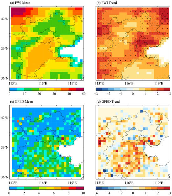
Figure 2.
Spatial patterns of the multi-year means ((a,c), units: days) and trends ((b), units: 10 a−1; (d), units: days 10 a−1) of the April–May fire weather index-based (a,b) and GFED-based wildfire days (c,d) in the BTH region.
Overall, regarding both the means and trends, the spatial patterns of the FWI-based and GFED-based wildfire days were similar, demonstrating that the FWI derived from climatic conditions could reflect wildfire events in the BTH region. However, there are still differences; for example, the northwestern BTH region exhibited high FWI values, while the GFED-based wildfire days did not indicate the occurrence of wildfire activity. This may be due to two factors: first, the remote sensing algorithms still exhibit significant uncertainties in recognizing wildfires; second, the high elevation in the northwestern parts of the BTH region causes high wind speeds and notable drought conditions, which may cause FWI overestimation, thereby distorting fire danger assessments.
3.2. SOM Analysis of the Fire Weather Index Composites
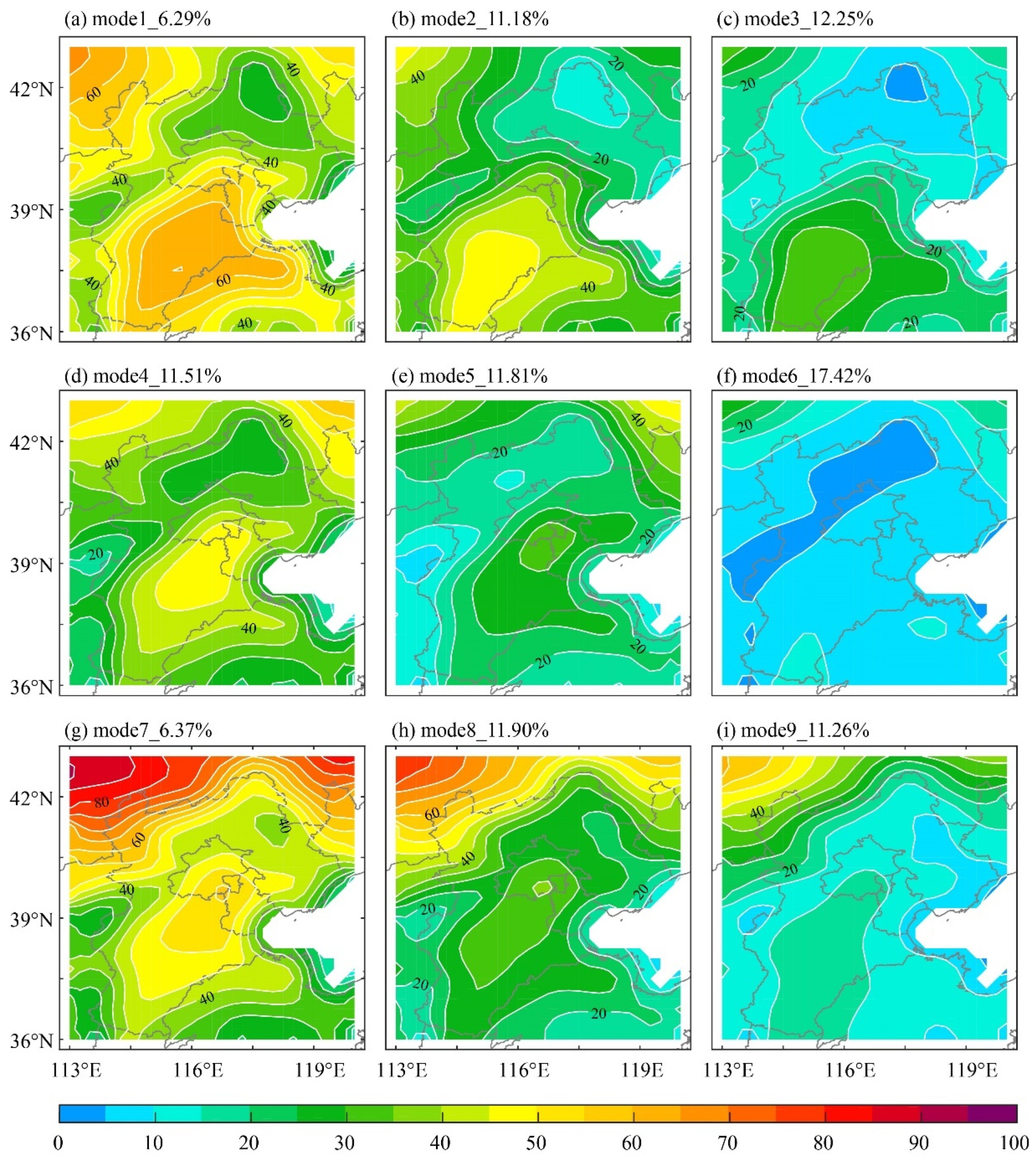
To identify dominant wildfire spatial patterns, we applied SOM analysis to the FWI dataset in the BTH region. Figure 3 shows a map of the nine mode patterns derived from SOM analysis of FWI composites. We found that the spatial patterns of the FWI for SOM modes 1, 2, 3, and 4 are similar, i.e., high values in the northwest and from the center to the south, with low values in the northeast. Moreover, the FWI intensity in the northwest and central regions is comparable to that in the southern region. The occurrence proportions of each SOM mode are 6.29%, 11.18%, 12.25%, and 11.51%, respectively. However, there are still differences in the locations of the high-FWI centers among these SOM modes. Notably, the high-FWI value of mode 1 is concentrated in the central to southern parts. However, the high-FWI value of mode 2 is concentrated in the southern part, while that of mode 4 is concentrated in the central part. The spatial pattern of the FWI for SOM mode 5 indicates high values in the central to eastern regions and low values in the western region, with the frequency reaching 11.81%. The spatial patterns of the FWI for SOM modes 7, 8, and 9 are similar, first decreasing and then increasing from northwest to southeast, with the highest FWI intensity in the northwestern region, which is higher than that in the central region. The frequency of each SOM mode is 6.37%, 11.90%, and 11.26%. Additionally, the spatial distribution of nonsignificant FWI values in the BTH region is represented by SOM mode 6. The abovementioned findings suggest that high FWI values occur in SOM modes 1, 2, 4, 7, and 8, but the high-concentration areas are not identical, indicating that the spatial patterns of wildfire occurrence vary.

Figure 3.
Nine mode patterns (a–i) derived from SOM analysis of FWI composites in the BTH region from 1981–2020 (the upper left corner value of each SOM mode indicates the percentage of occurrence of that pattern).
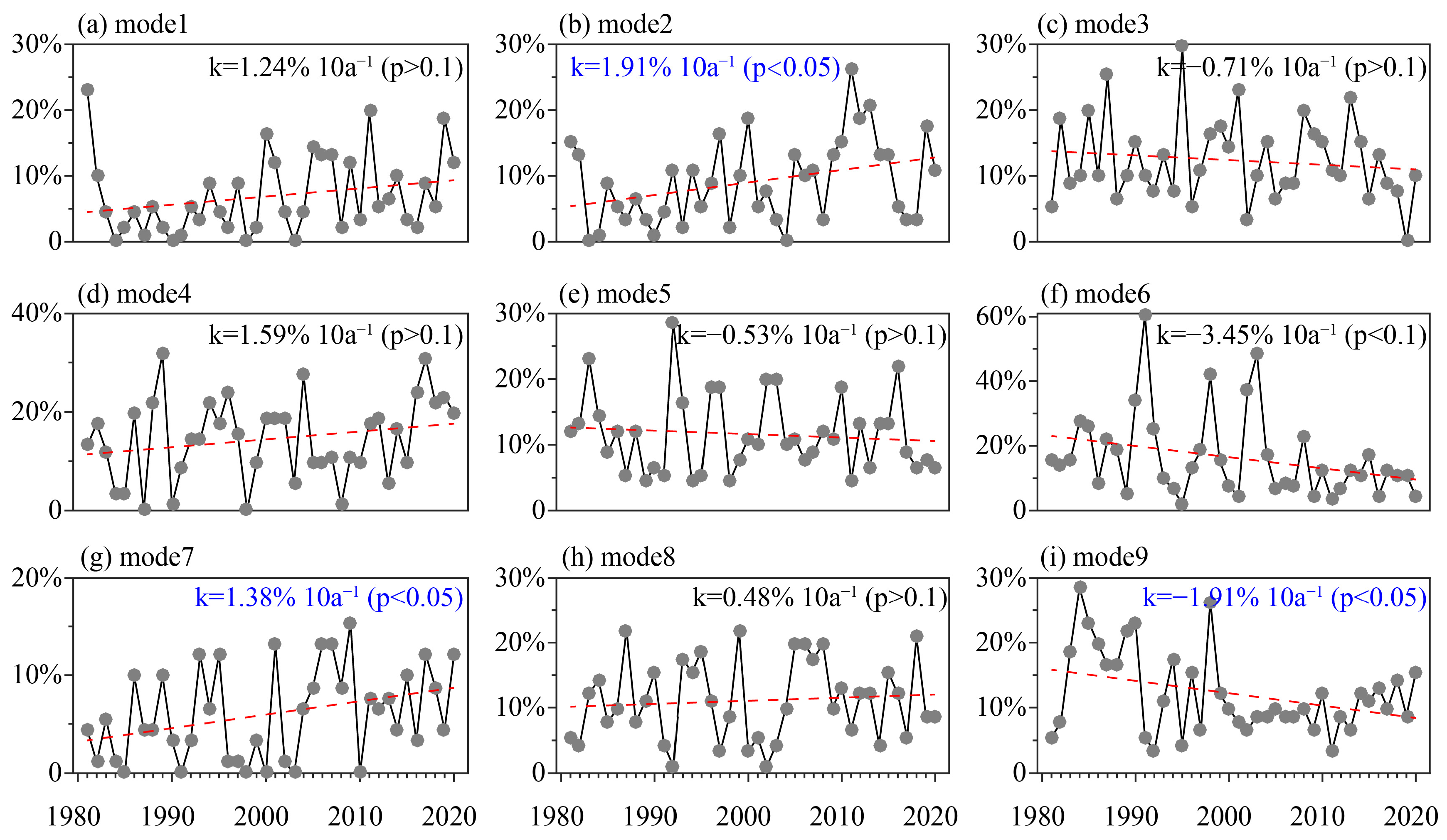
Through the temporal variations in the frequency of the SOM modes (Figure 4), we found that the frequency trends in SOM modes 1, 2, 4, 7, and 8 were positive, but only those of SOM modes 2 and 7 passed the 95% significance test, with frequency trends of 1.91% 10 a−1 and 1.38% 10 a−1, respectively. Moreover, the frequency trends of SOM modes 3, 5, 6, and 9 were negative, but only that of SOM mode 9 passed the 95% significance test, with a frequency trend of −1.91% 10 a−1. Considering that a high FWI exerts a greater impact on wildfires, we only analyzed SOM modes 2 and 7, which exhibited positive frequency trends, in the following study.
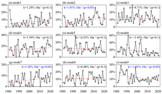
Figure 4.
Temporal variations in the frequency of nine SOM modes (a–i) over the past 40 years (the red dotted lines show the trend in the frequency of the SOM modes; k is the frequency variability per 10 years in each subplot; the blue values denote significance at a confidence level of 0.05).
3.3. Impact of Atmospheric Circulation Anomalies on the FWI
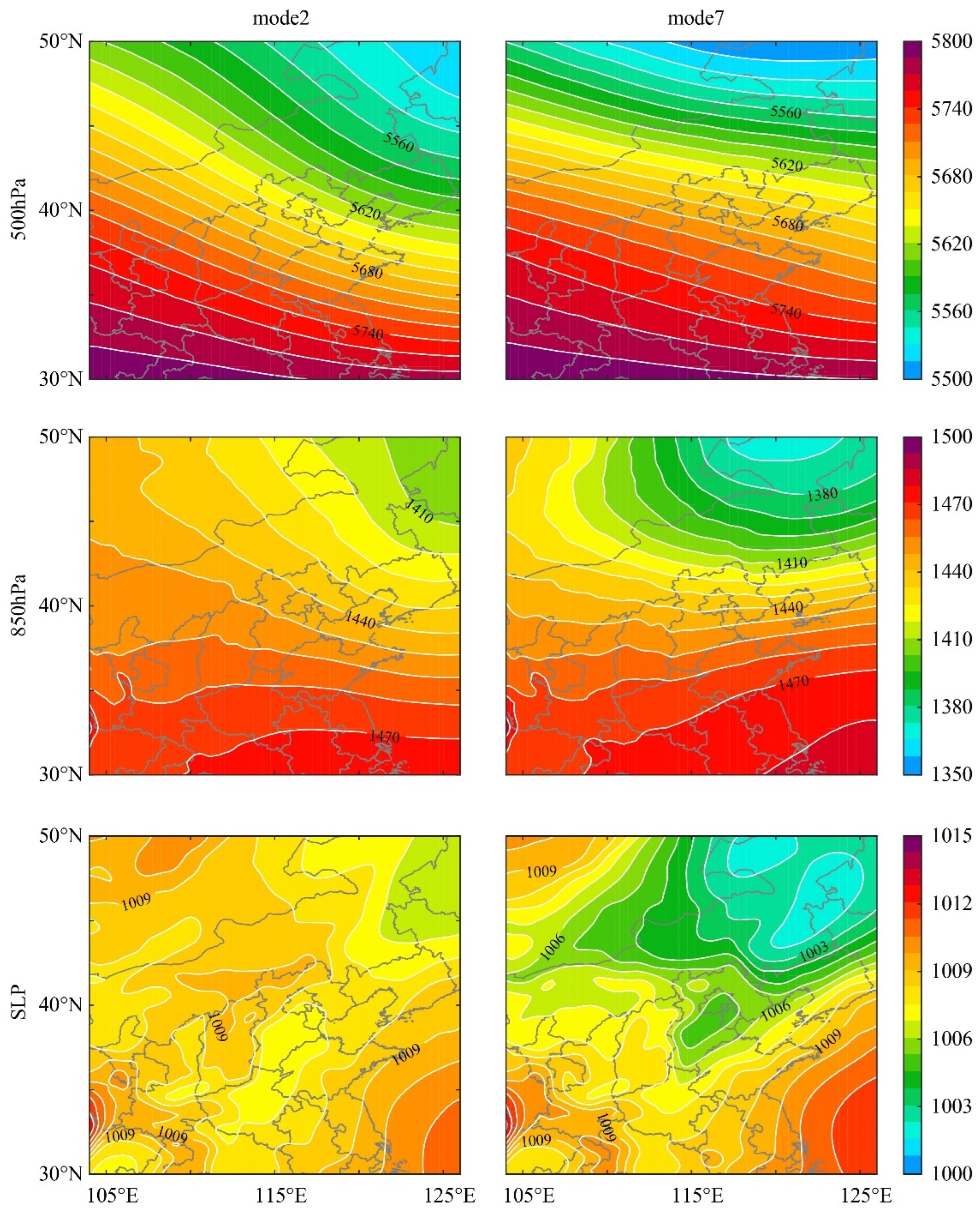
The weather type that drives wildfires cannot be attributed solely to one atmospheric circulation field because the factors that cause these events are complex and influenced by several weather variables. To research the linkage between atmospheric circulation and the FWI-derived SOM model, we selected the geopotential height at pressure levels of 500 and 800 hPa and sea level pressure on various FWI mode dates and calculated the ensemble mean (Figure 5). Through multiple atmospheric circulation elements, we determined the possible causes of wildfire occurrence.

Figure 5.
Spatial pattern of the geopotential height at pressure levels of 500 hPa (upper; units: m) and 850 hPa (middle; units: m) and sea-level pressure (bottom; units: hPa) composites in SOM modes 2 (left) and mode 7 (right).
The geopotential height at pressure levels of 500 and 850 hPa indicates that the BTH region occurs at a post-trough position with an anomalous low-pressure system to the northeast in FWI SOM mode 2. Under the influence of a post-trough front-ridge system, strong northerly winds from the northwest crossing high mountains may induce the Foehn effect, which can further rapidly intensify temperature increases and humidity decreases. These arid and rain-scarce conditions can further amplify the increase in FWI, thereby enhancing the trend of fire risk. For instance, Dong et al. (2021) [40] discovered that the Foehn wind effect along the eastern foothills of the Rocky Mountains could increase local fire spread rates by 67% under specific configurations of the 850 hPa wind field. Moreover, the sea level pressure field reveals that a weaker low-pressure system is formed in the southern region, and the eastern and western sides of this low-pressure system are controlled by high pressure, which in turn causes the weakening of the winds in the region. According to FWI SOM mode 7, at pressure levels of 500 and 850 hPa, the isobars are significantly pushed northward, and the absolute values are greater than those in SOM mode 2, even though the isobars in the BTH region are relatively flat. Under the control of this high-pressure system, the region exhibits high temperatures and drought weather conditions. Moreover, as indicated by the sea-level pressure, a significant low-pressure system is formed at the center of the BTH region, which is controlled by high pressure to the east and west, resulting in the weakening of the winds in this region.
The above-mentioned results demonstrate divergent meteorological drivers of high FWI values in SOM modes 2 and 7. In Mode 2, the southern BTH region experiences reduced moisture flux under a post-trough frontal ridge, while its northeastern sector is subject to strong pressure gradients driving persistent winds. Conversely, Mode 7’s central BTH high-FWI cluster arises from the dominance of a subtropical high-pressure ridge, which triggers adiabatic heating and prolonged drought. These findings underscore the need to incorporate synoptic-scale circulation diagnostics into fire risk prediction frameworks.
3.4. Contributions of the Fuel Available Index and Wildfire Spread Rate Index to the Fire Weather Index
To quantify the effects of the fuel available index and wildfire spread rate index on the FWI under the influence of atmospheric circulation, we derived partial differential equations of the FWI. Using the partial differential equations of the FWI, we calculated the relative contribution rates of the fuel available index and wildfire spread rate index at each grid cell in SOM modes 2 and 7 (Figure 6). We found that, in mode 2, the fuel available index, which contributes more than 50%, is the primary factor of the FWI variations in the central to southern BTH region. However, the wildfire spread rate index only contributes approximately 20%. The effect of the fuel available index on the FWI is more than twice that of the wildfire spread rate index. Additionally, the main factor influencing the FWI variations in the northeastern region is the wildfire spread rate index, which contributes approximately 40%. Similarly, the effect of the wildfire spread rate index on the FWI is twice that of the fuel available index. In SOM mode 7, the wildfire spread rate index only accounts for approximately 25% of the total FWI variation in the BTH region, while the fuel available index accounts for more than 50% of the total FWI variation. The effect of the fuel available index on the FWI variations is twice that of the wildfire spread rate index. Moreover, we found that in the high-elevation mountainous regions in the west and north, the contribution of the fuel available index to the FWI variations exceeded that of the wildfire spread rate index by a factor of approximately seven. This may be due to the high danger of wildfires triggered by the cumulative effect on vegetation over a long period due to factors such as drought caused by the lack of moisture influenced by the altitude.
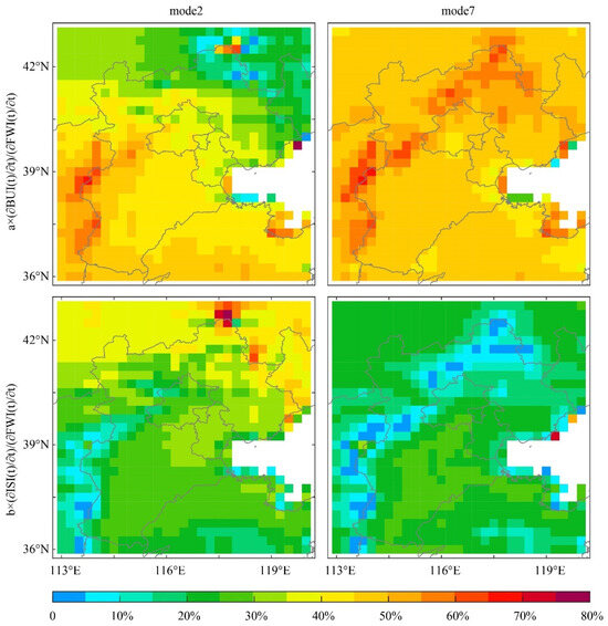
Figure 6.
Contribution rates of the BUI (upper; fuel available index calculated by Tmax, RH, and precipitation) and ISI (bottom; wildfire spread rate index calculated by WS) to the FWI in SOM mode 2 (left) and mode 7 (right).
The abovementioned findings suggest that, in mode 2, the fuel availability index is the dominant factor driving FWI variations in the central and southern regions, while the wildfire spread rate index predominates in the northeastern region. The FWI variations in the BTH region under mode 7 are influenced mainly by the fuel available index. These observations align with the spatial pattern of atmospheric circulation shown in Figure 6, which demonstrates that atmospheric circulation patterns influence local wildfire danger by modifying the fuel availability index and wildfire spread rate index in different modes, respectively. It is important to note that the sum of the contributions from the variations in the fuel available index and the wildfire spread rate index does not total 100%. There are two aspects. On the one hand, we implement an approximate transformation when calculating the partial differential equations, as shown in Figure 2. On the other hand, the derived partial differential equation contains a residual term, which, although negligible, could still affect the results.
4. Discussion
4.1. The Composites of Fire Weather Index Anomaly Under the Different SSP Scenarios
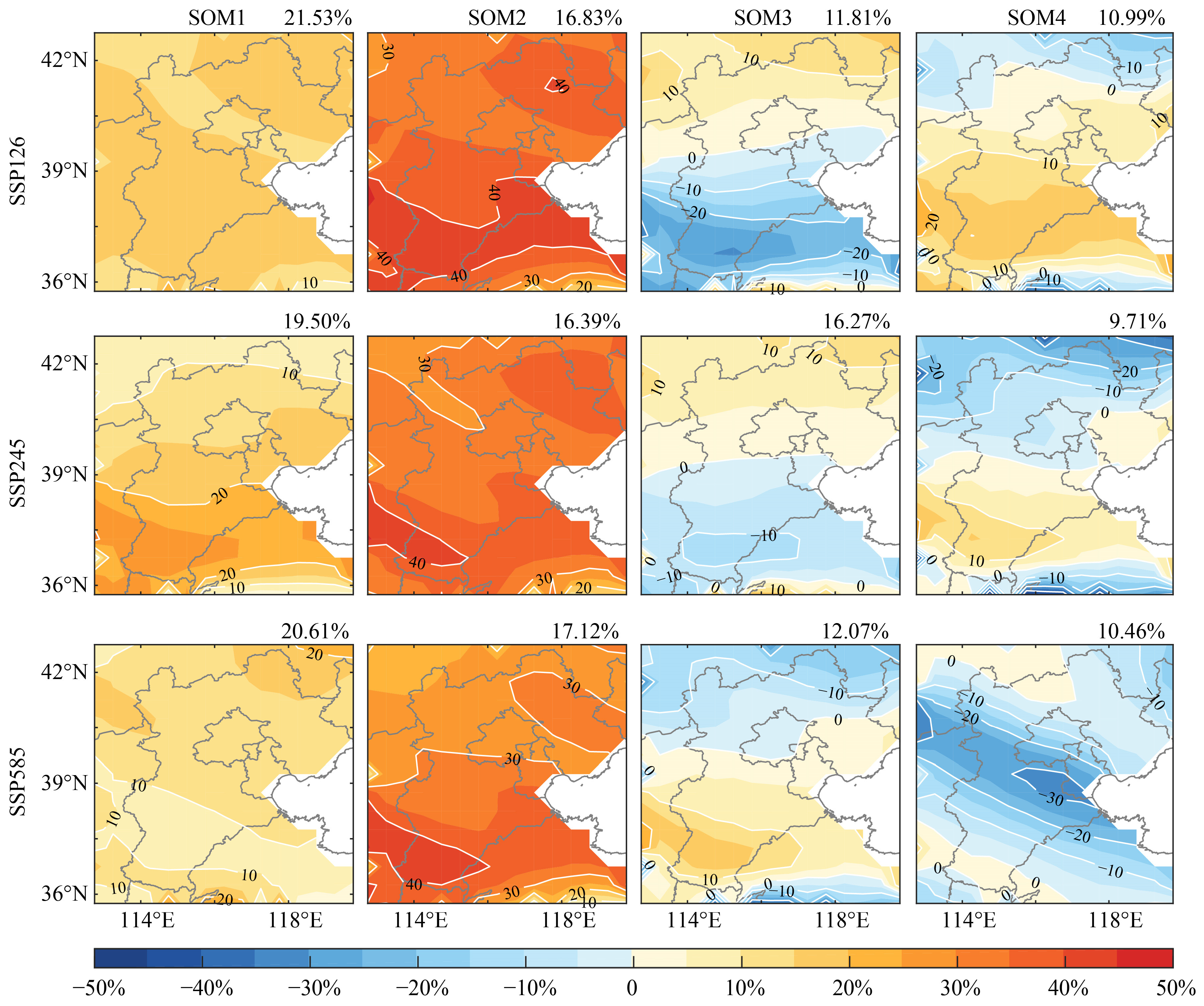
Figure 7 illustrates the top four SOM modes of the composites of FWI anomaly percentages in the BTH region under the SSP126, SSP245, and SSP585 scenarios. The spatial patterns of the four SOM modes of the FWI exhibit variations across the different SSP scenarios. In the SSP126 scenario, SOM1 and SOM2, which both displayed notable increases in FWI anomaly percentages, had similar spatial patterns; their frequencies were 21.53% and 16.83%, respectively. Notably, the intensity of FWI in SOM2 was stronger than that in SOM1. The highest values in SOM2 were in the northeast and south of the BTH region with an average increase of more than 35%. With 39° N as its border, the spatial pattern of SOM3 is “north increase–south decrease”. Except for a few northern regions, SOM4 represented an increase in FWI intensity throughout the majority of the BTH region. The south of Hebei showed the strongest increasing tendency, with an average increase of almost 15%. In the SSP245 scenario, the spatial patterns of FWI anomalies percentage of SOM1, SOM2, and SOM3 were consistent with those in SSP126. It is noted that the intensity of FWI was particularly significant in SOM2, with an average increase of more than 35%. The spatial pattern of SOM4, in contrast to SOM3, was characterized by “north decrease–south increase”. In the SSP585 scenario, the spatial patterns of FWI anomalies percentage of SOM1 and SOM2 were consistent with those in SSP126. However, spatial patterns of SOM1 between SSP585 and SSP126 differed somewhat, with the primary difference being that SSP585’s FWI was more concentrated in the northern region of the BTH region. The spatial pattern of SOM3, characterized by “north decrease–south increase”, was largely consistent with SOM4 of SSP245. The primary feature of the FWI SOM4 is a decline throughout the BTH region, with the central portion in the central region of the BTH region.
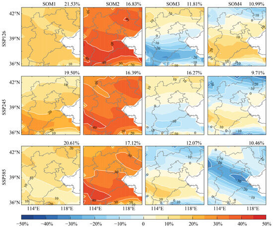
Figure 7.
The composites of FWI anomalies percentage for the top four mode patterns derived from SOM analysis in the BTH region from 2021–2100 under the SSP126 (top), SSP245 (middle), and SSP585 scenarios (bottom) (the reference period is from 1981 to 2020; the upper right corner value of each SOM mode indicates the percentage of occurrence of that pattern).
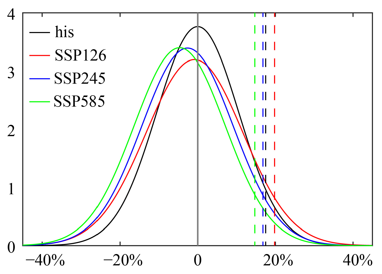
Figure 8 illustrates the differences in the probability density function pattern of the regional mean FWI anomalies percentage at an annual scale in the BTH region among the historical period and three SSP scenarios. We found that the regional average FWI fell for all SSP scenarios as compared to the historical period. This implied that, although we discovered various regional patterns of fire danger in the BTH region, the climatology mean was characterized by a decline in FWI intensity. In terms of the 95% quantile, the intensity of the extreme FWI was greater for SSP126 than for the historical period but decreased for SSP245 and SSP585, which might mean some connection to FWI regionalization.
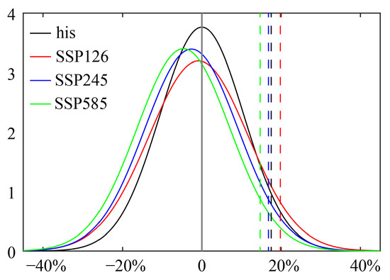
Figure 8.
Probability density function pattern of regional mean FWI anomalies percentage at an annual scale in the BTH region between the historical period and three SSP scenarios (the reference period is from 1981 to 2020; the dotted lines indicate 95th percentile).
The abovementioned findings suggested that the top two SOM modes with the highest frequency, irrespective of the SSP scenario, were characterized by an increasing FWI in the BTH region; nevertheless, there were some differences in the centers of FWI variations. The frequencies of the top two SOM modes are all close to 40% of the total. However, for all SSP scenarios, the annual-scale intensity of the regional mean FWI in the BTH region declined in comparison to the historical period. Only for SSP126 were the FWI extremes (95% quartile) greater than they were during the historical period. For the other two scenarios, though they became less significant compared with the historical period, SSP585 has the most pronounced decline than SSP245. This implied that FWI displayed different characteristics at various time scales; hence, going forward, we should take time-scale variability into account when making predictions about FWI.
4.2. The Application of the SOM in Classifying Wildfire Patterns
The application of Self-Organizing Maps (SOMs) in identifying fire weather patterns is gaining momentum. By leveraging their capabilities in dimensionality reduction and clustering, SOMs have effectively revealed the nonlinear coupling mechanisms between weather systems and wildfire events. This technique allows for the identification of critical fire weather patterns through unsupervised learning of multidimensional meteorological data, organizing similar patterns into a continuous matrix. A notable case study demonstrated the efficacy of coupling SOM with the WRF model to analyze meteorological phenomena in geographically complex environments [40]. Their findings revealed that under specific synoptic configurations characterized by distinct 850 hPa wind field patterns, the localized fire propagation velocity could experience a statistically significant amplification of up to 67%. This atmospheric dynamic interaction underscores the critical role of topographically induced wind regimes in modulating wildfire behavior within mountainous terrain ecosystems. In Mediterranean Spain, these methodologies facilitated the characterization of meteorological conditions conducive to fire ignition through the identification of recurrent weather patterns associated with extreme fire danger [41]. Similarly, along the North American Pacific Northwest, SOM-based analyses elucidated key environmental drivers governing wildfire propagation dynamics by mapping complex relationships between atmospheric variables and combustion processes [42]. A comparative analysis of three weather pattern classification techniques—composite analysis, EOF analysis, and SOM—was conducted to identify weather patterns associated with large wildfires in the Pacific Northwest of the United States. The results indicated that the SOM approach can capture more transitional weather patterns, which holds significant value for wildfire risk assessment [43]. This technique facilitates the identification of regional fire danger archetypes and their associated weather signatures, thereby enhancing the predictive capacity for extreme fire events in this climatically sensitive region. The integration of SOM-derived insights into operational forecasting frameworks could significantly improve the accuracy and lead time of wildfire warnings, ultimately aiding in the development of more effective fire management strategies for North China’s ecosystems.
5. Conclusions
In this study, we investigated the impact of climate change on different FWI SOM modes in the BTH region, identifying nine distinct spatial patterns of the FWI through SOM analysis. Our results revealed an increasing trend in the frequency of two SOM modes (modes 2 and 7) over the past four decades. The spatial patterns showed that the highest FWI values are observed in the southern and central regions in SOM modes 2 and 7, respectively. Further analysis of atmospheric circulation suggested that the increase in fuel availability, and consequently in FWI, is respectively driven by a post-trough system that leads to reduced water vapor movement in SOM mode 2 and a high-pressure system causing elevated temperatures and drought-like conditions in SOM mode 7, respectively. We quantified the contributions of the BUI and the ISI to the FWI using partial differential derivation for the first time. The highest FWI values in both the southern and central regions for SOM modes 2 and 7 were predominantly influenced by variations in the Fuel-Available index. Regardless of the SSP scenario, we found that the top two SOM modes with the highest frequency were consistently associated with an increasing FWI trend in the BTH region. However, for all SSP scenarios, the regional mean FWI intensity on an annual scale showed a decline compared to the historical period. Only under the SSP126 scenario did the FWI extremes (95th percentile) surpass historical levels, while for the other two SSP scenarios, these extremes became less pronounced. These findings implied the importance of accounting for time-scale variability when predicting FWI trends. Our study highlighted the need for enhanced attribution analysis techniques to improve future wildfire monitoring efforts, thereby enabling a more nuanced understanding of wildfire responses to ongoing climate change. In addition to the impact of climate conditions, local land-use changes can impact the FWI by modifying fuel availability and moisture levels. For instance, urbanization tends to reduce vegetation cover, leading to lower fuel loads and potentially decreasing FWI values. In contrast, afforestation or reforestation can enhance fuel continuity and moisture retention, which may result in an increase in FWI. Additionally, agricultural practices like irrigation can affect soil moisture, subsequently influencing FWI levels. By analyzing fire risk trends and causes, effective assistance can be provided to government departments in implementing relevant preventive measures for high fire risks. These measures include strengthening fire source control by strictly prohibiting smoking in forest areas; improving the monitoring and early warning systems through the use of satellite remote sensing and drone patrols for real-time fire monitoring; enhancing public education and awareness by disseminating fire prevention knowledge through multiple channels to raise public awareness of fire prevention; and reinforcing infrastructure construction by perfecting firebreaks and fire-fighting passages and ensuring an adequate supply of fire-fighting equipment.
Author Contributions
Conceptualization, M.W., W.D. and C.Z. (Caishan Zhao); methodology, M.W., C.Z. (Caishan Zhao), W.D. and C.Z. (Chengpeng Zhang); software, C.Z. (Chengpeng Zhang), M.L. and J.C.; formal analysis, M.W., W.D. and C.Z. (Chengpeng Zhang); data curation, C.Z. (Chengpeng Zhang) and M.L.; writing—original draft preparation, M.W. and W.D.; writing—review and editing, C.Z. (Caishan Zhao). All authors have read and agreed to the published version of the manuscript.
Funding
This research was funded by the National Key R&D Program of China, grant number 2023YFC320660103 (funder: M.W.), Innovation and Development Special Foundation of the China Meteorological Administration: CXFZ2025J068 (funder: W.D.), and the Science and Technology Project of Beijing Institute of Emergency Management Science and Technology, grant number YJ2024044 (funder: W.D.).
Institutional Review Board Statement
Not applicable.
Informed Consent Statement
Not applicable.
Data Availability Statement
All data used in this study are publicly available and can be downloaded from the corresponding websites. The GFED v4.1 used in this study can be archived at https://www.geo.vu.nl/~gwerf/GFED/GFED4/, accessed on 10 March 2024. The hourly ERA5 global reanalysis meteorological data were provided by the ECMWF (https://cds.climate.copernicus.eu/datasets/reanalysis-era5-pressure-levels-monthly-means?tab=overview, accessed on 20 July 2024). The global climate model data used in this study can be obtained from the CMIP6 archives at https://esgf-node.llnl.gov/search/cmip6/, accessed on 1 June 2024.
Conflicts of Interest
The authors declare no conflicts of interest.
References
- Knorr, W.; Arneth, A.; Jiang, L. Demographic controls of future global fire risk. Nat. Clim. Chang. 2016, 61, 781–787. [Google Scholar] [CrossRef]
- Hudiburg, T.; Mathias, J.; Bartowitz, K.; Berardi, D.M.; Bryant, K.; Graham, E.; Kolden, C.A.; Betts, R.A.; Lynch, L. Terrestrial carbon dynamics in an era of increasing wildfire. Nat. Clim. Chang. 2024, 13, 1306–1316. [Google Scholar] [CrossRef]
- Chinese Academy of Science. Blue Book of Forest Fire Carbon Emissions Research. 2023. Available online: http://www.iae.cas.cn/gb2019/xwzx_156509/ttxw_156510/202312/P020231212296936577850.pdf (accessed on 1 March 2024). (In Chinese).
- Williams, A.P.; Abatzoglou, J.T.; Gershunov, A.; Guzman-Morales, J.; Bishop, D.A.; Balch, J.K.; Lettenmaier, D.P. Observed Impacts of Anthropogenic Climate Change on Wildfire in California. Earths Future 2019, 7, 892–910. [Google Scholar] [CrossRef]
- Jain, P.; Castellanos-Acuna, D.; Coogan, S.C.P.; Abatzoglou, J.T.; Flannigan, M.D. Observed increases in extreme fire weather driven by atmospheric humidity and temperature. Nat. Clim. Chang. 2021, 12, 63–72. [Google Scholar] [CrossRef]
- McDowell, N.G.; Allen, C.D. Darcy’s law predicts widespread forest mortality under climate warming. Nat. Clim. Change 2015, 5, 669–672. [Google Scholar] [CrossRef]
- Touma, D.; Stevenson, S.; Lehner, F.; Coats, S. Human-driven greenhouse gas and aerosol emissions cause distinct regional impacts on extreme fire weather. Nat. Commun. 2021, 12, 212. [Google Scholar] [CrossRef]
- Tomasevic, I.C.; Vucetic, V.; Cheung, K.K.W.; Fox-Hughes, P.; Beggs, P.J.; Prtenjak, M.T.; Malecic, B. Comparison of Meteorological Drivers of Two Large Coastal Slope-Land Wildfire Events in Croatia and South-East Australia. Atmosphere 2023, 14, 1076. [Google Scholar] [CrossRef]
- Chaparro, D.; Piles, M.; Vall-Llossera, M.; Camps, A. Surface moisture and temperature trends anticipate drought conditions linked to wildfire activity in the Iberian Peninsula. Eur. J. Remote Sens. 2017, 49, 955–971. [Google Scholar] [CrossRef]
- Chen, L.F.; Dou, Q.; Zhang, Z.M.; Shen, Z.H. Moisture content variations in soil and plant of post-fire regenerating forests in central Yunnan Plateau, Southwest China. J. Geogr. Sci. 2019, 29, 1179–1192. [Google Scholar] [CrossRef]
- Abatzoglou, J.T.; Williams, A.P. Impact of anthropogenic climate change on wildfire across western US forests. Proc. Natl. Acad. Sci. USA 2016, 113, 11770–11775. [Google Scholar] [CrossRef]
- Goss, M.; Swain, D.L.; Abatzoglou, J.T.; Sarhadi, A.; Kolden, C.A.; Williams, A.P.; Diffenbaugh, N.S. Climate change is increasing the likelihood of extreme autumn wildfire conditions across California. Environ. Res. Lett. 2020, 15, 094016. [Google Scholar] [CrossRef]
- Kirchmeier-Young, M.C.; Zwiers, F.W.; Gillett, N.P.; Cannon, A.J. Attributing extreme fire risk in Western Canada to human emissions. Clim. Chang. 2017, 144, 365–379. [Google Scholar] [CrossRef] [PubMed]
- Tian, X.R.; Shu, L.F.; Zhao, F.J.; Wang, M.Y. Impacts of climate change on forest fire danger in China. Sci. Silvae Sin. 2017, 53, 159–169. [Google Scholar] [CrossRef]
- Bai, M.X.; Du, W.P.; Wu, M.W.; Zhang, C.P.; Xing, P.; Hao, Z.X. Variation in fire danger in the Beijing-Tianjin-Hebei region over the past 30 years and its linkage with atmospheric circulation. Clim. Chang. 2024, 177, 27. [Google Scholar] [CrossRef]
- Ding, Y.H.; Wang, Z.Y.; Sun, Y. Inter-decadal variation of the summer precipitation in East China and its association with decreasing Asian summer monsoon. Part I: Observed evidences. Int. J. Climatol. 2008, 28, 1139–1161. [Google Scholar] [CrossRef]
- Ding, Y.H.; Sun, Y.; Wang, Z.Y.; Zhu, Y.X.; Song, Y.F. Inter-decadal variation of the summer precipitation in China and its association with decreasing Asian summer monsoon Part II: Possible causes. Int. J. Climatol. 2009, 29, 1926–1944. [Google Scholar] [CrossRef]
- Liu, Y.Z.; Wu, C.Q.; Jia, R.; Huang, J.P. An overview of the influence of atmospheric circulation on the climate in arid and semi-arid region of Central and East Asia. Sci. China Earth Sci. 2018, 61, 1183–1194. [Google Scholar] [CrossRef]
- Dong, Q.; Sun, J.; Chen, B.Y.; Chen, Y.; Shu, Y. Similarities of Three Most Extreme Precipitation Events in North China. Atmosphere 2023, 14, 1149. [Google Scholar] [CrossRef]
- Yang, Q.R.; Jiang, C.; Ding, T. Impacts of Extreme-High-Temperature Events on Vegetation in North China. Remote Sens. 2023, 15, 4542. [Google Scholar] [CrossRef]
- Du, W.P.; Hao, Z.X.; Bai, M.X.; Zhang, L.; Zhang, C.P.; Wang, Z.R.; Xing, P. Spatiotemporal Variation in the Meteorological Drought Comprehensive Index in the Beijing-Tianjin-Hebei Region during 1961–2023. Water 2024, 15, 4230. [Google Scholar] [CrossRef]
- Bai, M.X.; Du, W.P.; Hao, Z.X.; Zhang, L.; Xing, P. The characteristics and future projections of fire danger in the areas around mega-city based on meteorological data–a case study of Beijing. Front. Earth Sci. 2024, 18, 637–648. [Google Scholar] [CrossRef]
- Van Wagner, C.E. Development and Structure of the Canadian Forest Fire Weather Index System; Canadian Forest Search Technology Report; Petawawa National Forestry Institute, Canadian Forest Service: Chalk River, ON, Canada, 1987. [Google Scholar]
- Laneve, G.; Pampanoni, V.; Shaik, R.U. The Daily Fire Hazard Index: A Fire Danger Rating Method for Mediterranean Areas. Remote Sens. 2020, 12, 2356. [Google Scholar] [CrossRef]
- Field, R.D. Evaluation of Global Fire Weather Database reanalysis and short-term forecast products. Nat. Hazards Earth Syst. Sci. 2020, 20, 1123–1147. [Google Scholar] [CrossRef]
- McElhinny, M.; Beckers, J.F.; Hanes, C.; Flannigan, M.; Jain, P. A high-resolution reanalysis of global fire weather from 1979 to 2018-overwintering the Drought Code. Earth Syst. Sci. Data 2020, 12, 1823–1833. [Google Scholar] [CrossRef]
- Hersbach, H.; Bell, B.; Berrisford, P.; Hirahara, S.; Horányi, A.; Muñoz-Sabater, J.; Nicolas, J.; Peubey, C.; Radu, R.; Schepers, D.; et al. The ERA5 global reanalysis. Q. J. R. Meteorol. Soc. 2020, 146, 1999–2049. [Google Scholar] [CrossRef]
- Choudhury, D.; Ji, F.; Nishant, N.; Di Virgilio, G. Evaluation of ERA5-Simulated Temperature and Its Extremes for Australia. Atmosphere 2023, 14, 913. [Google Scholar] [CrossRef]
- Dhmane, L.A.; Moustadraf, J.; Rachdane, M.; Saidi, M.E.; Benjmel, K.; Amraoui, F.; Ezzaouini, M.A.; Sliman, A.A.; Hadri, A. Spatiotemporal Assessment and Correction of Gridded Precipitation Products in North Western Morocco. Atmosphere 2023, 14, 1239. [Google Scholar] [CrossRef]
- Ramon, J.; Lledo, L.; Torralba, V.; Soret, A.; Doblas-Reyes, F.J. What global reanalysis best represents near-surface winds? Q. J. R. Meteorol. Soc. 2019, 145, 3236–3251. [Google Scholar] [CrossRef]
- Beck, H.E.; Pan, M.; Roy, T.; Weedon, G.P.; Pappenberger, F.; van Dijk, A.I.J.M.; Huffman, G.J.; Adler, R.F.; Wood, E.F. Daily evaluation of 26 precipitation datasets using Stage-IV gauge-radar data for the CONUS. Hydrol. Earth Syst. Sci. 2019, 23, 207–224. [Google Scholar] [CrossRef]
- van der Werf, G.R.; Randerson, J.T.; Giglio, L.; van Leeuwen, T.T.; Chen, Y.; Rogers, B.M.; Mu, M.Q.; van Marle, M.J.E.; Morton, D.C.; Collatz, G.J.; et al. Global fire emissions estimate during 1997–2016. Earth Syst. Sci. Data 2017, 9, 697–720. [Google Scholar] [CrossRef]
- Zhang, T.R.; Wooster, M.J.; de Jong, M.C.; Xu, W.D. How Well Does the “Small Fire Boost” Methodology Used within the GFED4.1s Fire Emissions Database Represent the Timing, Location and Magnitude of Agricultural Burning? Remote Sens. 2018, 10, 823. [Google Scholar] [CrossRef]
- Andela, N.; Morton, D.C.; Giglio, L.; Paugam, R.; Chen, Y.; Hantson, S.; van der Werf, G.R.; Randerson, J.T. The Global Fire Atlas of individual fire size, duration, speed and direction. Earth Syst. Sci. Data 2019, 11, 529–552. [Google Scholar] [CrossRef]
- Pinto, G.A.S.J.; Rousseu, F.; Niklasson, M.; Drobyshev, I. Effects of human-related and biotic landscape features on the occurrence and size of modern forest fires in Sweden. Agric. For. Meteorol. 2020, 291, 108084. [Google Scholar] [CrossRef]
- Wastl, C.; Schunk, C.; Leuchner, M.; Pezzatti, G.B.; Menzel, A. Recent climate change: Long-term trends in meteorological forest fire danger in the Alps. Agric. For. Meteorol. 2012, 162, 1–13. [Google Scholar] [CrossRef]
- Grillakis, M.; Voulgarakis, A.; Rovithakis, A.; Seiradakis, K.D.; Koutroulis, A.; Field, R.D.; Kasoar, M.; Papadopoulos, A.; Lazaridis, M. Climate drivers of global wildfire burned area. Environ. Res. Lett. 2022, 17, 045021. [Google Scholar] [CrossRef]
- Johnson, N.C.; Feldstein, S.B.; Tremblay, B. The Continuum of Northern Hemisphere Teleconnection Patterns and a Description of the NAO Shift with the Use of Self-Organizing Maps. J. Clim. 2008, 21, 6354–6371. [Google Scholar] [CrossRef]
- Kohonen, T. Essentials of the self-organizing map. Neural Netw. 2013, 37, 52–65. [Google Scholar] [CrossRef]
- Dong, L.; Leung, L.R.; Qian, Y.; Zou, Y.F.; Song, F.F.; Chen, X.D. Meteorological Environments Associated with California Wildfires and Their Potential Roles in Wildfire Changes During 1984–2017. J. Geophys. Res. Atmos. 2021, 126, e2020JD033180. [Google Scholar] [CrossRef]
- Rodrigues, M.; González-Hidalgo, J.C.; Peña-Angulo, D.; Jiménez-Ruano, A. Identifying wildfire-prone atmospheric circulation weather types on mainland Spain. Agric. For. Meteorol. 2019, 264, 92–103. [Google Scholar] [CrossRef]
- Trouet, V.; Taylor, A.H.; Carleton, A.M.; Skinner, C.N. Fire-climate interactions in forests of the American Pacific coast. Geophys. Res. Lett. 2006, 33, 1–5. [Google Scholar] [CrossRef]
- Zhong, S.Y.; Yu, L.J.; Heilman, W.E.; Bian, X.D.; Fromm, H. Synoptic weather patterns for large wildfires in the northwestern United States-a climatological analysis using three classification methods. Theor. Appl. Climatol. 2020, 141, 1057–1073. [Google Scholar] [CrossRef]


Disclaimer/Publisher’s Note: The statements, opinions and data contained in all publications are solely those of the individual author(s) and contributor(s) and not of MDPI and/or the editor(s). MDPI and/or the editor(s) disclaim responsibility for any injury to people or property resulting from any ideas, methods, instructions or products referred to in the content. |
© 2025 by the authors. Licensee MDPI, Basel, Switzerland. This article is an open access article distributed under the terms and conditions of the Creative Commons Attribution (CC BY) license (https://creativecommons.org/licenses/by/4.0/).