The Correlation Between Surface Temperature and Surface PM_2.5 in Nanchang Region, China

Abstract

PM_2.5 plays a significant role in urban climate, especially as urban development accelerates. In this study, surface PM_2.5, skin temperature, surface air temperature, net longwave radiation, net shortwave radiation, sensible heat flux, and latent heat flux were directly analyzed in Nanchang from 2020 to 2022. The results indicate that PM_2.5 in Nanchang is highest during winter and lowest in summer. On an annual scale, surface PM_2.5 reduces skin and surface air temperatures at a rate of 0.75 °C/(μg m⁻³) by decreasing net solar radiation and increasing net longwave radiation at night. Conversely, it increases air temperature by absorbing radiation, leading to a surface inversion. Furthermore, surface PM_2.5 influences surface air and skin temperatures by modulating the latent heat fluxes.

1. Introduction

PM_2.5 is one of the major air pollutants in Chinese cities, primarily emitted from fossil fuel combustion in industrial areas and anthropogenic emissions in densely populated regions. It significantly affects local air quality, human health, and regional and global climate [1,2,3,4]. Due to its small size, persistence, and significant environmental impacts, PM_2.5 has attracted considerable attention from the public and the scientific community [5]. Meteorological factors are known to influence the dispersion, dilution, aggregation, and retention of PM_2.5, thereby affecting its concentration in the air [6,7,8]. Specifically, wind is the main driver of PM_2.5 transport [9], high relative humidity can increase PM_2.5 [10], and precipitation effectively reduces PM_2.5 [11]. A robust inversion layer and low mixing height can compress pollutants near the surface, leading to elevated PM_2.5 [12]. While the influence of meteorological factors on PM_2.5 is well documented, the impact of PM_2.5, especially at higher concentrations, on local meteorology and climate remains incompletely understood.

PM_2.5 refers to fine particulate matter with an aerodynamical diameter of less than 2.5 μm. The scattering and absorption of solar radiation by these particles directly affects the radiative balance of the Earth’s atmospheric system, leading to changes in solar radiation, temperature, wind speed, and boundary layer height [13,14,15]. The accumulation of particulate matter brings the heated atmosphere closer to the surface, altering the energy flux and thereby affecting atmospheric stability and reducing atmospheric inversions [16]. Im et al. [17] concluded that small differences in PM_2.5 during the summer months can lead to changes in air temperature. Cao et al. [18] argued that elevated particulate matter concentrations may contribute to urban heat islands at night, due to increased incoming longwave radiation. In contrast, observations by Wu et al. [19,20] suggest that increases in urban PM_2.5 tend to reduce urban heat island intensity. Therefore, the effect of PM_2.5 on local urban temperatures is variable and requires further investigation.

The absorption of solar radiation by PM_2.5 redistributes heat in the convective boundary layer, influencing the thermal properties of the surface layer [21]. However, this impact is not consistent. For example, in offshore China, PM_2.5 contributes to the warming of the surface atmospheric layer and induces atmospheric instability [22], whereas in the Jing-Jin-Ji region, PM_2.5 enhances the strength of the inversion layer [23]. Studies on the effects of PM_2.5 on the climate of the surface layer tend to concentrate on specific regions or large cities, such as North China, the Pearl River Delta, Xi’an, and Nanjing [24,25,26]. The results can differ based on the region, season, and climatic conditions, underscoring the necessity for observational studies across regions to more comprehensively elucidate the effects of PM_2.5 on surface temperature.

Nanchang is one of the hottest cities in China, with a historically high summer temperature of 40.9 °C. Therefore, studying the relationship between surface PM_2.5 and surface temperature in Nanchang throughout the year, and elucidating the mechanism based on continuous observational data, can improve our understanding of the impact of PM_2.5 on local surface meteorological conditions. This, in turn, can help decision-makers formulate more effective prevention strategies.

2. Data and Methods

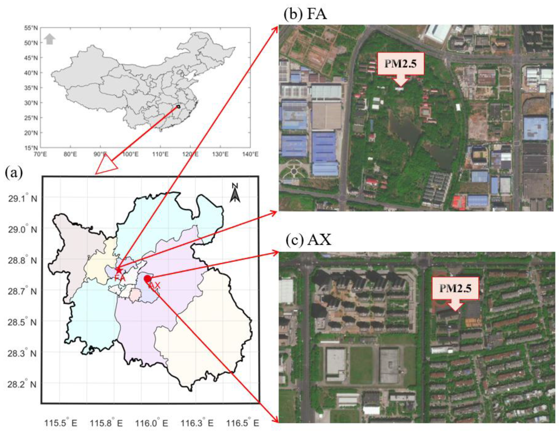
2.1. PM_2.5 Observations

PM_2.5 concentrations were collected over a span of three years, from 2020 to 2022, at the Jiangxi Forestry Academy Station (28°44.72′ N, 115°49.57′ E; referred to as FA) and the Aixi Lake Station (28°42.33′ N, 115°59.02′ E; referred to as AX) in Nanchang (28°10′–29°11′ N, 115°27′–116°35′ E; Figure 1). Nanchang is located in the north–central region of Jiangxi Province, in East China, and falls within the subtropical monsoon climate zone. The city comprises six districts and three counties, covering a total area of 7195 km². As of the end of 2022, it had a permanent resident population of 6.54 million, with a forest cover of 22.0%. Nanchang has an average annual temperature of 17 °C to 17.7 °C and an average annual relative humidity of 78.5%. Both stations are located in the central part of Nanchang, surrounded by buildings and vegetation. However, the area surrounding FA is characterized by lush vegetation, with buildings that are not high (~15 m) and are relatively scattered, as well as small ponds.

PM_2.5 concentrations were measured using a Thermo Scientific Inc (Massachusetts, USA). Tapering Element Oscillation Microbalance (TEOM) 1405-DF analyzer. The analyzer was installed in a temperature-controlled enclosure on the roof of a building at each site to reduce the impact of vehicle emissions. It calculated the concentrations of particulate matter by detecting changes in the oscillation frequency of a conical glass element as particles settled on a filter positioned at the tip of the element. The instrument automatically determined concentrations that included both non-volatile and volatile PM components using the Filter Dynamics Measurement System (FDMS). To capture and retain both non-volatile and volatile PM, the FDMS directed the sample flow through a cooled filter maintained at 4 °C. The FDMS valve alternated every six minutes, switching between the deposition of sample particles on the TEOM filters and the flow of clean air through the TEOM filters [27]. The instrument complies with the technical specifications for PM measurements set by the Chinese Environmental Protection Administration. Quality control checks were performed every 15 days and included inspection of the enclosure, replacement of filters, calibration of flow rates, and cleaning of the sample inlet. In-line filters were replaced semi-annually, and the dryer was replaced annually. Hourly average PM_2.5 data were output and stored at each site.

2.2. Meteorological Data

We selected the hourly meteorological variable field, surface energy flux, and radiation from ERA5 (the fifth major global reanalysis produced by ECMWF; Hersbach et al. [28]), including 2 m air temperature, skin temperature, mean net shortwave radiation, mean net longwave radiation, mean surface latent heat flux, and mean surface sensible heat flux. The ambient meteorological data were interpolated to PM_2.5 locations using the inverse distance weight (IDW) method.

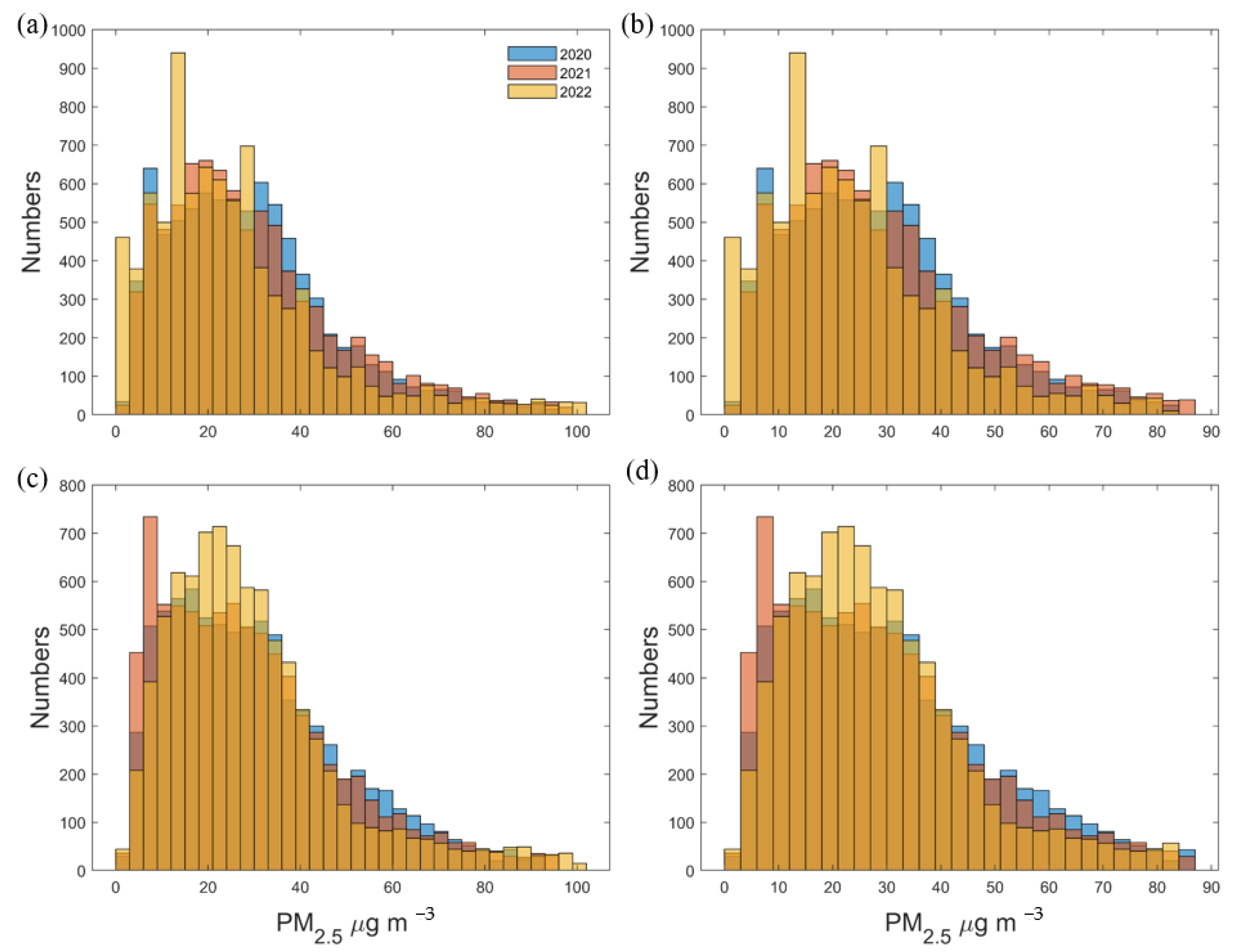
2.3. PM_2.5 Data Quality

The following sequential steps were used for quality control of PM_2.5 in this study: (1) data were removed during manual maintenance according to the maintenance records, (2) NAN values present in the observations were excluded, (3) PM_2.5 values of less than 0 and the number of PM_2.5 exceeding the extreme value (100 μg m⁻³ in this study) were excluded, and, (4) according to the distribution law of the normal distribution, |X_i − X_m|>3σ data (X_i is the vector data of PM_2.5, X_m is the averaged PM_2.5, σ is the stand deviation) were also rejected.

The distribution histogram of PM_2.5 before and after quality control is shown in Figure 2. The data post-quality control generally indicate that the PM_2.5 maximum is less than 90 μg m⁻³, and PM_2.5 is primarily within the range of 10 μg m⁻³ to 30 μg m⁻³, suggesting that PM_2.5 levels are low and air quality is good most of the time. However, it is also evident that when PM_2.5 exceeds 40 μg m⁻³, its frequency is higher at AX sites than at FA sites, implying variability in the distribution of PM_2.5 in Nanchang. The standard deviations of the PM_2.5 observations are 2.4 μg m⁻³ in spring, 1.4 μg m⁻³ in summer, 2.8 μg m⁻³ in autumn, and 2.5 μg m⁻³ in winter in FA and 2.3 μg m⁻³ in spring, 2.0 μg m⁻³ in summer, 2.6 μg m⁻³ in autumn, and 2.5 μg m⁻³ in winter in AX.

2.4. Linear Regression and Regression Analysis

Linear regression is used to analyze the relationship between factor Y and factor X. For a series of observations of Y, it can be expressed as a linear function of X, represented as Y = b × X + b₀. The coefficients b and b₀ can be determined using the least-squares method, where b signifies the slope of the linear function, and it can be calculated as:

$$b={\displaystyle \frac{n\sum x_i{y}_i-\sum x_i\sum y_i}{n\sum x_i^2-{\left(\sum x_i\right)}^2}}$$

(1)

A positive slope indicates that the value of factor Y increases as X changes, while a negative slope suggests a decreasing trend over time. Linear regression can predict the dependent variable by fitting a straight line, which has strong predictive power. Additionally, the coefficients and intercepts in linear regression can be interpreted as a weighted relationship between the independent and dependent variables, offering strong interpretability.

To test the statistical significance, we estimated the p-value using a two-tailed Student’s t-test, with the effective degrees of freedom calculated according to Bretherton et al. [29]. The Student’s t-test assumes that the distributions of the two populations have equal but unknown variances and that each population is normally distributed. The t-statistic (T) follows a t-distribution with a degree of freedom (df) of (n1 + n2 − 2). The further T is from zero, the less likely it is for such a value of T to be observed, indicating a greater variance between the groups. If T is too large, the null hypothesis will be rejected. The probability of rejecting the null hypothesis when it is actually true was determined (significance level α = 0.05). In general, the p-value represents the probability that a sample result would lead to the null hypothesis being true. Therefore, if the p-value is lower than the significance level, the null hypothesis can be rejected.

3. Results and Discussion

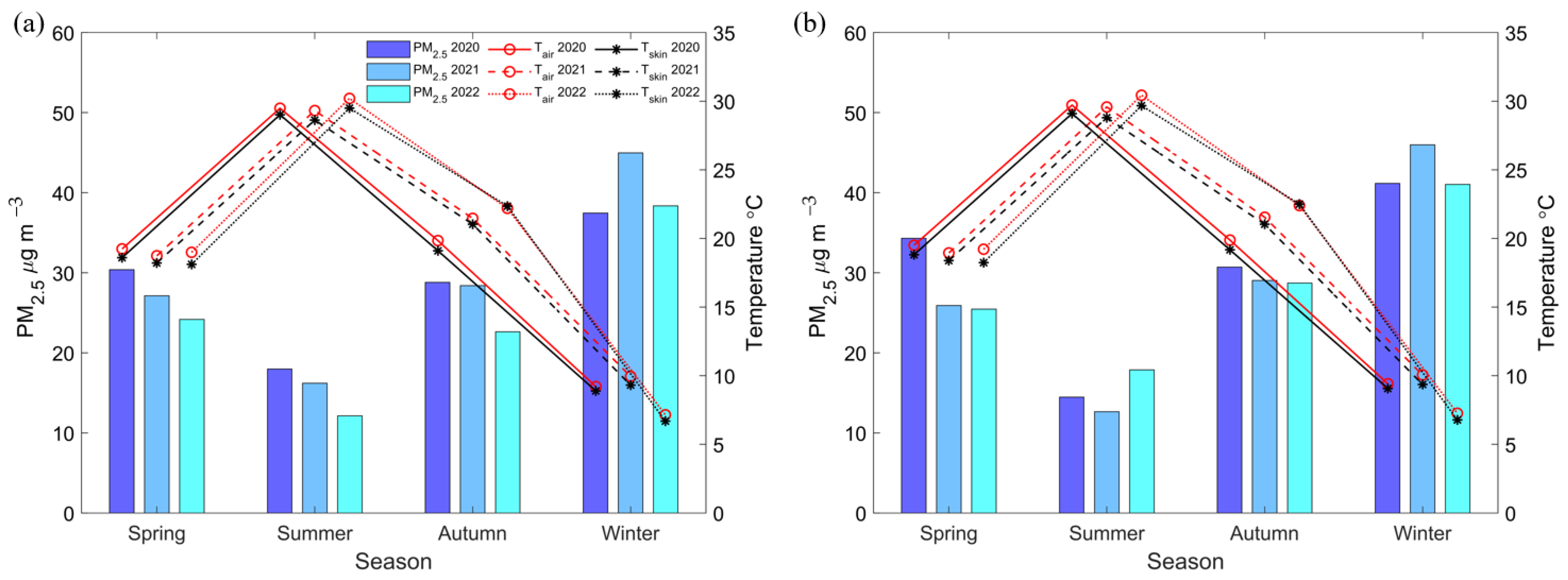
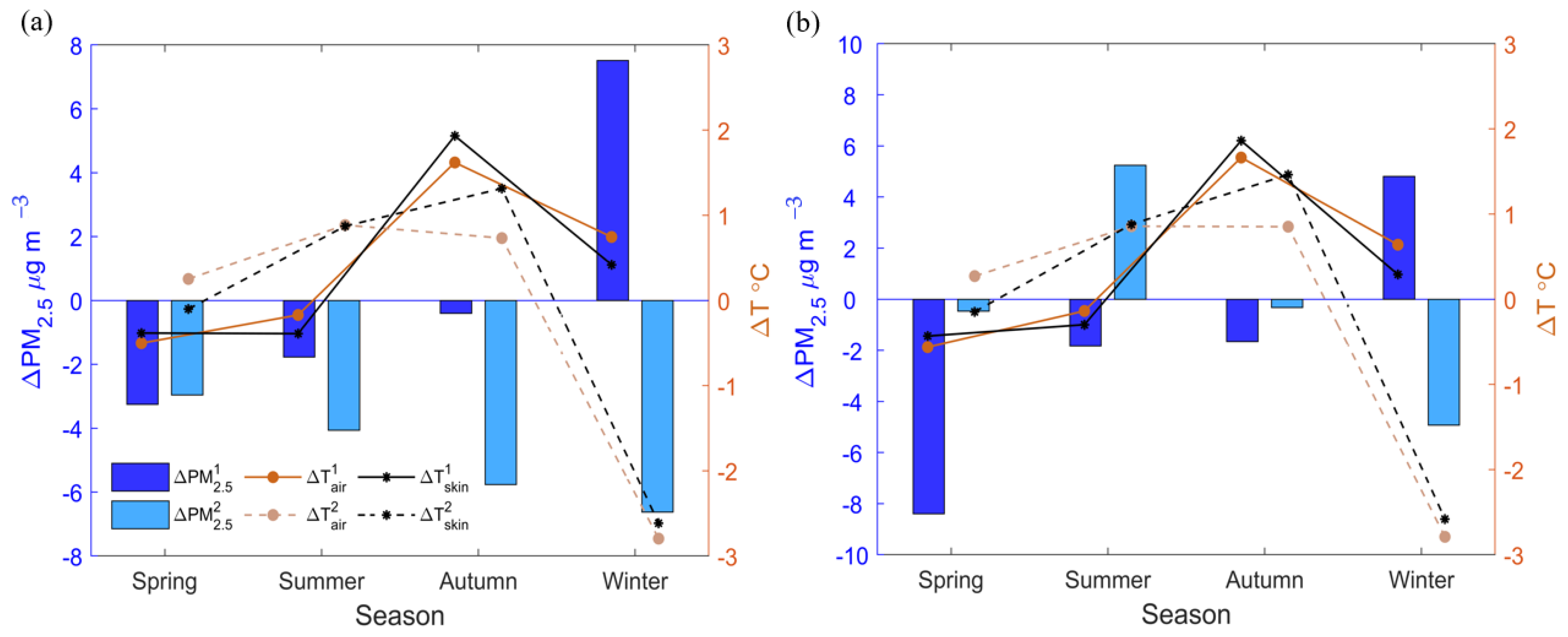
3.1. Seasonal Variations of Surface PM_2.5 and Surface Temperature

PM_2.5 in FA and AX showed the lowest values of 15.4 and 14.9 μg m⁻³ during the summer, whereas they reached their peak values of 40.25 and 42.7 μg m⁻³ in winter (Figure 3). Overall, surface temperature displayed a pattern of higher values in summer and lower values in winter, indicating a clear seasonal variation. This result is consistent with the seasonal variation of PM_2.5 reported in other southern cities, e.g., Louie et al. [30], but it contrasts with findings from the Jing-Jin-Ji urban agglomeration [31,32]. The main reason for this discrepancy can be attributed to the fact that PM_2.5 sources in the Jing-Jin-Ji urban agglomeration are predominantly influenced by soil dust, coal combustion, biomass burning, traffic and waste incineration emissions, industrial pollution, and secondary inorganic aerosols [15,32].

During spring, skin temperature (T_skin) at both the FA and the AX sites decreased as surface PM_2.5 levels dropped, yet surface air temperature (T_air) did not exhibit a significant trend during this period. In contrast, both T_air and T_skin increased with the reduction in surface PM_2.5 in autumn. During the summer and winter, fluctuations in both T_air and T_skin were noted in relation to the surface PM_2.5 at each site. The PM_2.5 at the FA site in the summers of 2020, 2021, and 2022 was 17.98 μg m⁻³, 16.20 μg m⁻³, and 12.14 μg m⁻³, respectively, corresponding to a T_air of 29.48 °C, 29.31 °C, and 30.19 °C, respectively. The PM_2.5 at AX during this period was 14.47 μg m⁻³, 12.64 μg m⁻³, and 17.88 μg m⁻³, corresponding to a T_air of 29.71 °C, 29.57 °C, and 30.43 °C, respectively. In winter, both FA and AX indicated that a higher PM_2.5 correlated with higher temperatures. Overall, surface temperature and PM_2.5 exhibited a negative correlation, suggesting that PM_2.5 can weaken the solar radiation reaching the surface, which in turn leads to a decrease in T_skin and T_air. This is consistent with the finds of Liao et al. [33], Song et al. [34], and Gao et al. [35], who demonstrated that a higher PM_2.5 can reduce T_air by 0.8–2.8 °C. However, our study also indicates that the impact of PM_2.5 variations on surface temperature in Nanchang does not consistently increase or decrease seasonally, which may be attributed to the source or composition of PM_2.5 [5,31,32]. Nonetheless, this is beyond the scope of this article. Consequently, we propose that the effects of surface PM_2.5 on surface temperature in Nanchang are complex and multifaceted.

The difference in surface PM_2.5 levels between the same season in two consecutive years (ΔPM_2.5) had a greater influence on ΔT_air than on ΔT_skin (Figure 4). For example, the surface PM_2.5 in spring 2021 was 3.25 μg m⁻³ lower than in 2020, corresponding to a decrease of 0.38 °C in T_skin and of 0.5 °C in T_air. In 2022, the surface PM_2.5 was 2.96 μg m⁻³ lower than in 2021, resulting in a decrease of 0.1 °C in T_skin and an increase of 0.25 °C in T_air. The influence of surface PM_2.5 on T_skin was greater than that on T_air in autumn. For example, in autumn 2021, the surface PM_2.5 was 1.66 μg m⁻³ lower than in 2020, corresponding to an increase of 1.86 °C in T_skin and an increase of 1.66 °C in T_air. In autumn 2022, the surface PM_2.5 was 0.33 μg m⁻³ lower than in 2021, which corresponded to a 1.46 °C increase in T_skin and a 0.85 °C increase in T_air. This indicates that changes in surface PM_2.5 can lead to local surface temperature variations.

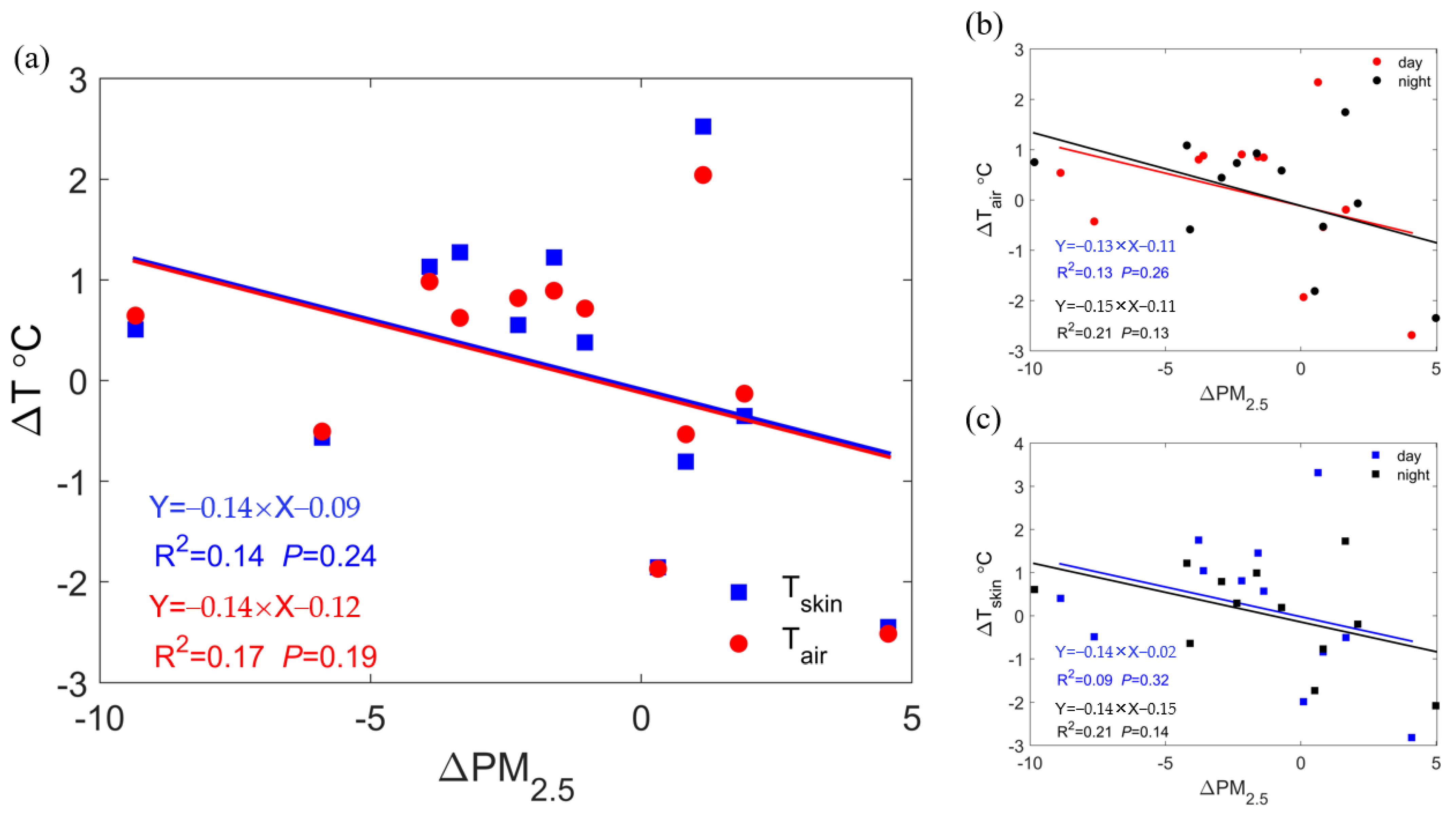
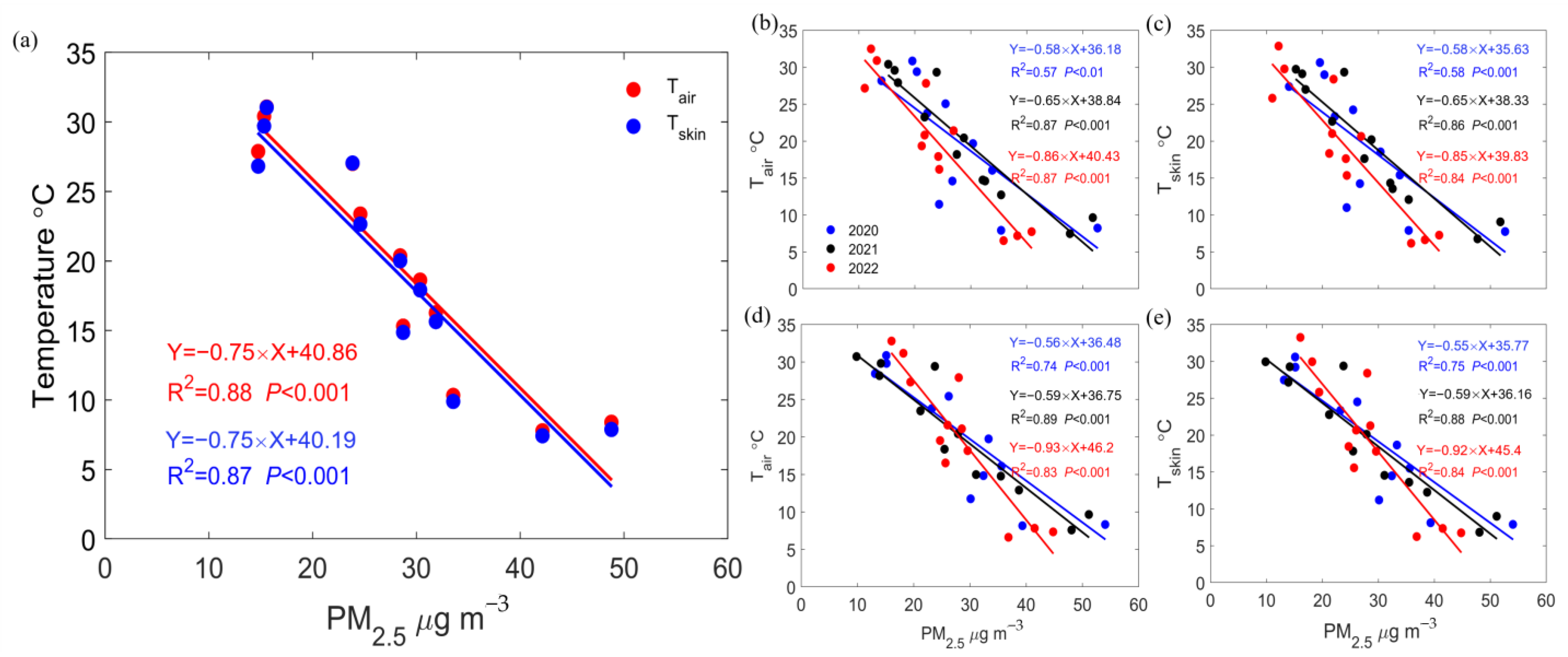
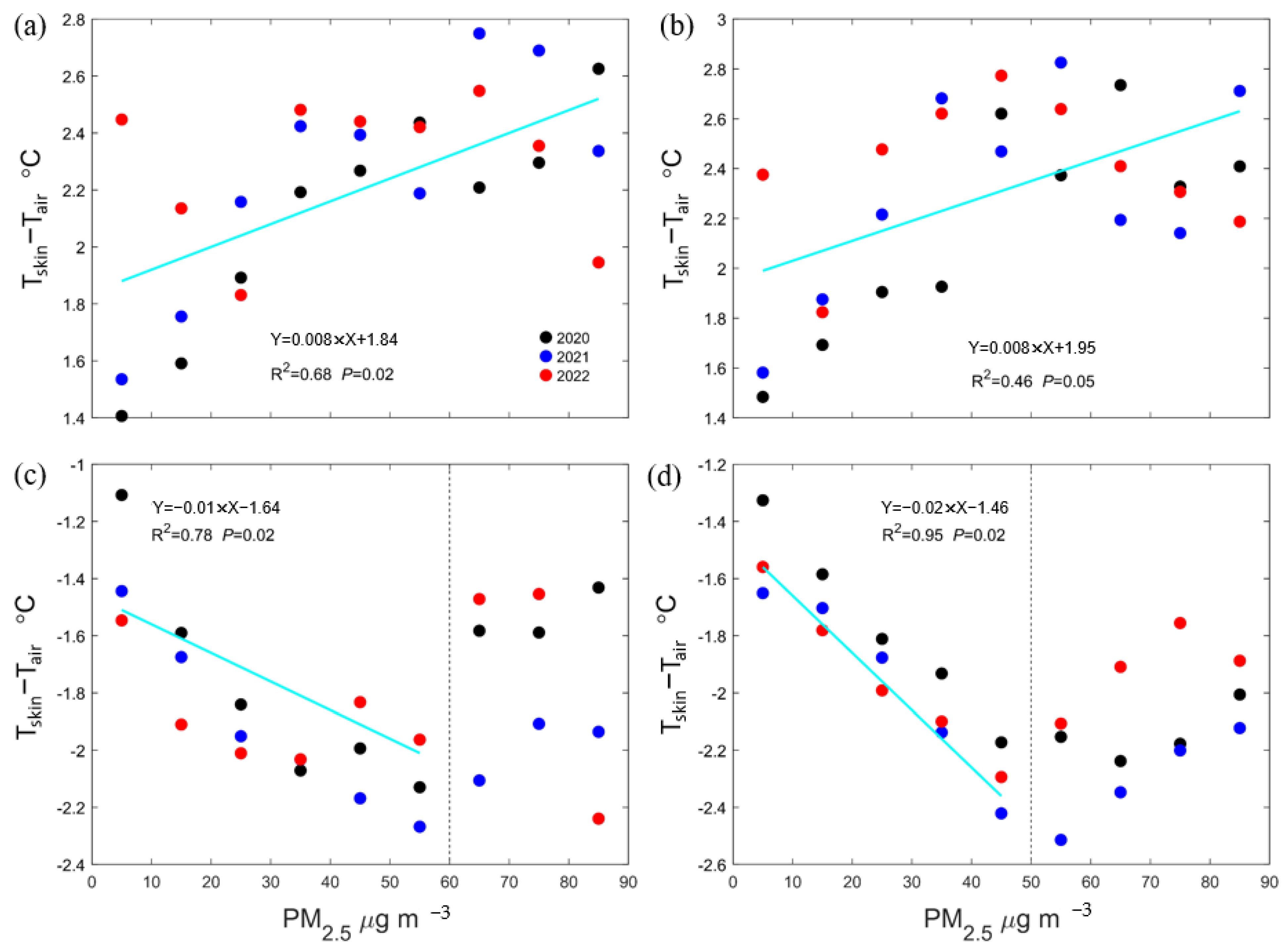
3.2. Response of Local Surface Temperature to PM_2.5 Concentrations

The relationship between PM_2.5 and both T_air and T_skin was very strong (R² > 0.8, p < 0.001, Figure 5a). Temperature decreased significantly with increasing PM_2.5 at a rate of 0.75 °C/(μg m⁻³) on an annual scale. The rate of decrease for T_air was 0.58 °C/(μg m⁻³) and 0.65 °C/(μg m⁻³), and for T_skin, it was 0.56 °C/(μg m⁻³) and 0.59 °C/(μg m⁻³) (Figure 5b–e). However, in 2022, when the PM_2.5 was lower, the rate of decrease in T_air and T_skin at FA was 0.86 °C/(μg m⁻³) and 0.85 °C/(μg m⁻³), respectively (Figure 5b,c), while at AX it was 0.93 °C/(μg m⁻³) and 0.92 °C/(μg m⁻³) (Figure 5d,e). This indicates that, on an annual scale, PM_2.5 has a significant impact on both skin and air temperatures.

The rate of decrease in monthly ΔT_air during the day and at night was 0.14 °C/(μg m⁻³), and the rate of decrease in ΔT_skin was the same during the day and at night. However, both correlations were poor (p > 0.1, Figure A1). Interestingly, the decrease observed at night appeared to be more favorable than during the day, suggesting that PM_2.5 might affect surface air temperature more than skin temperature. There was a weak correlation between PM_2.5 and the difference between T_skin and T_air (p > 0.6, R² < 0.1) on a monthly scale (Figure 6). The skin temperature was lower than the air temperature (T_skin − T_air < 0), leading to an inversion near the surface. However, the relationship between this inversion and PM_2.5 was not significant (p > 0.6, R² < 0.1) on monthly scale. This indicates that an increase in PM_2.5 did not alter the intensity of the inversion but may have contributed to its persistence on monthly scale. The conclusion that PM_2.5 can cause an inversion is also supported by research on cities in northern China [14,23,25]. Particulate matter is thought to decrease the skin temperature by reducing solar radiation and increase air temperature by absorbing or backscattering solar radiation, which is the reason for the inversion [12].

We further analyzed the relationship between the difference between T_skin and T_air and PM_2.5 (Figure 7). When there was no inverse (T_sink > T_air), the difference between T_sink and T_air increased significantly (p ≤ 0.05) with increasing PM_2.5. When an inverse (T_sink < T_air) was present, the inverse tended to increase with the increase in PM_2.5, but this increase seemed to decrease when PM_2.5 reached a certain level. For example, the inversion at FA was strongest when PM_2.5 was 60 μg m⁻³, while it was strongest when AX was 50 μg m⁻³. Similarly, at AX, when there was no inversion, there was a slight downward trend in PM_2.5 above 50 μg m⁻³, but this did not occur at the FA site. This implies that there is a difference in the effect of PM_2.5 on temperature in suburban and urban areas.

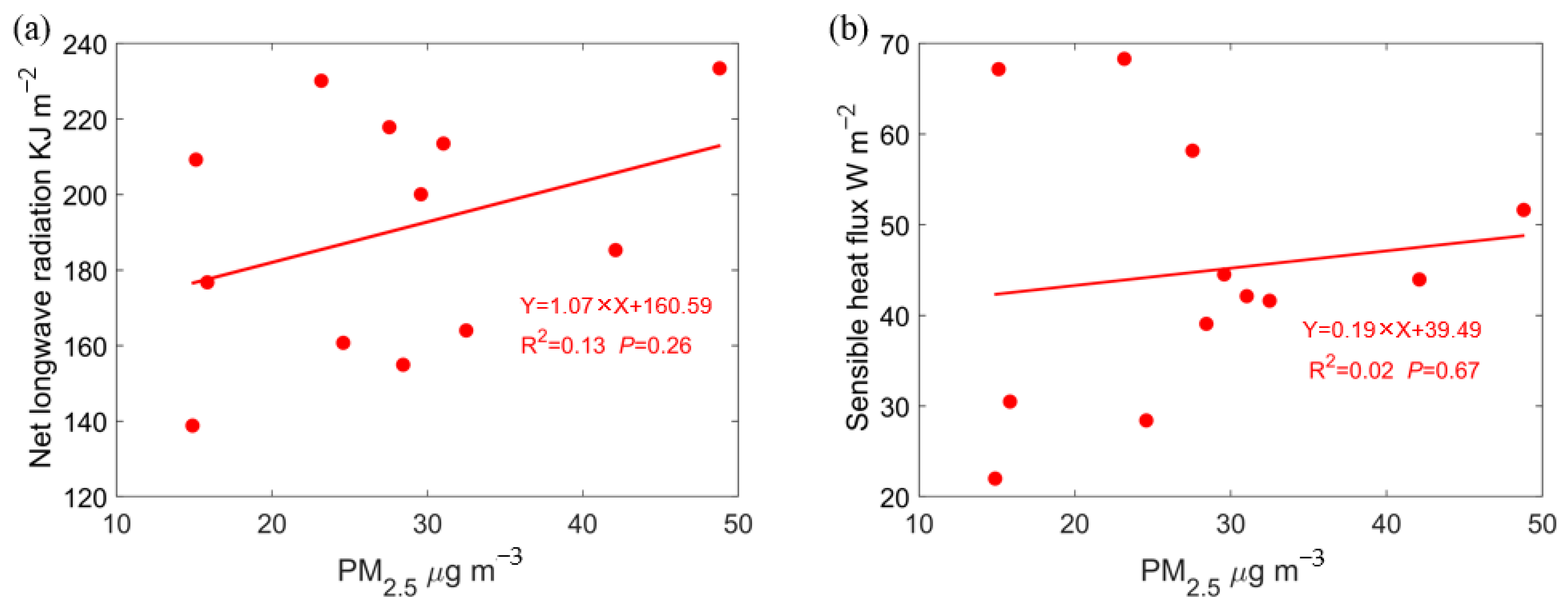
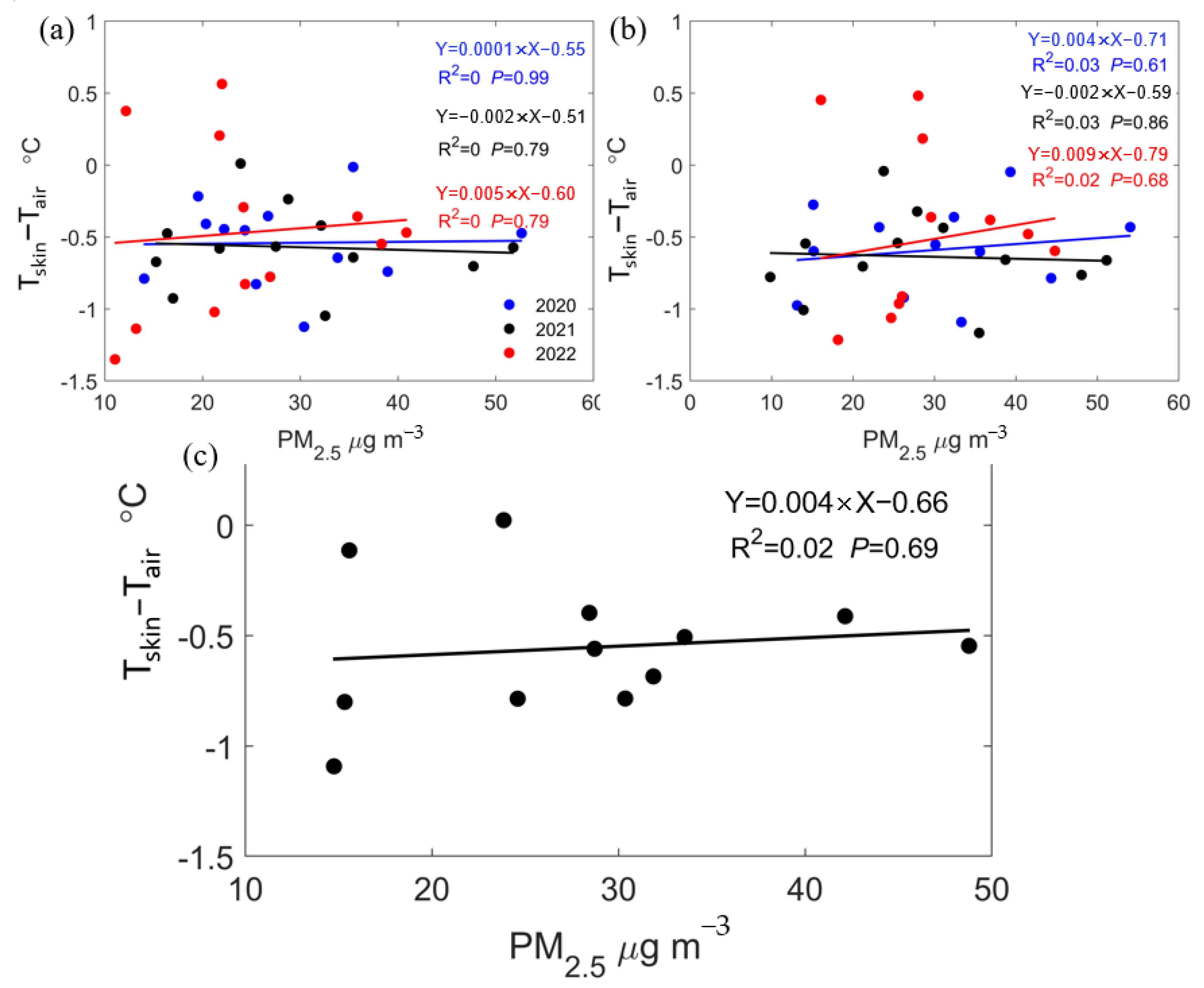
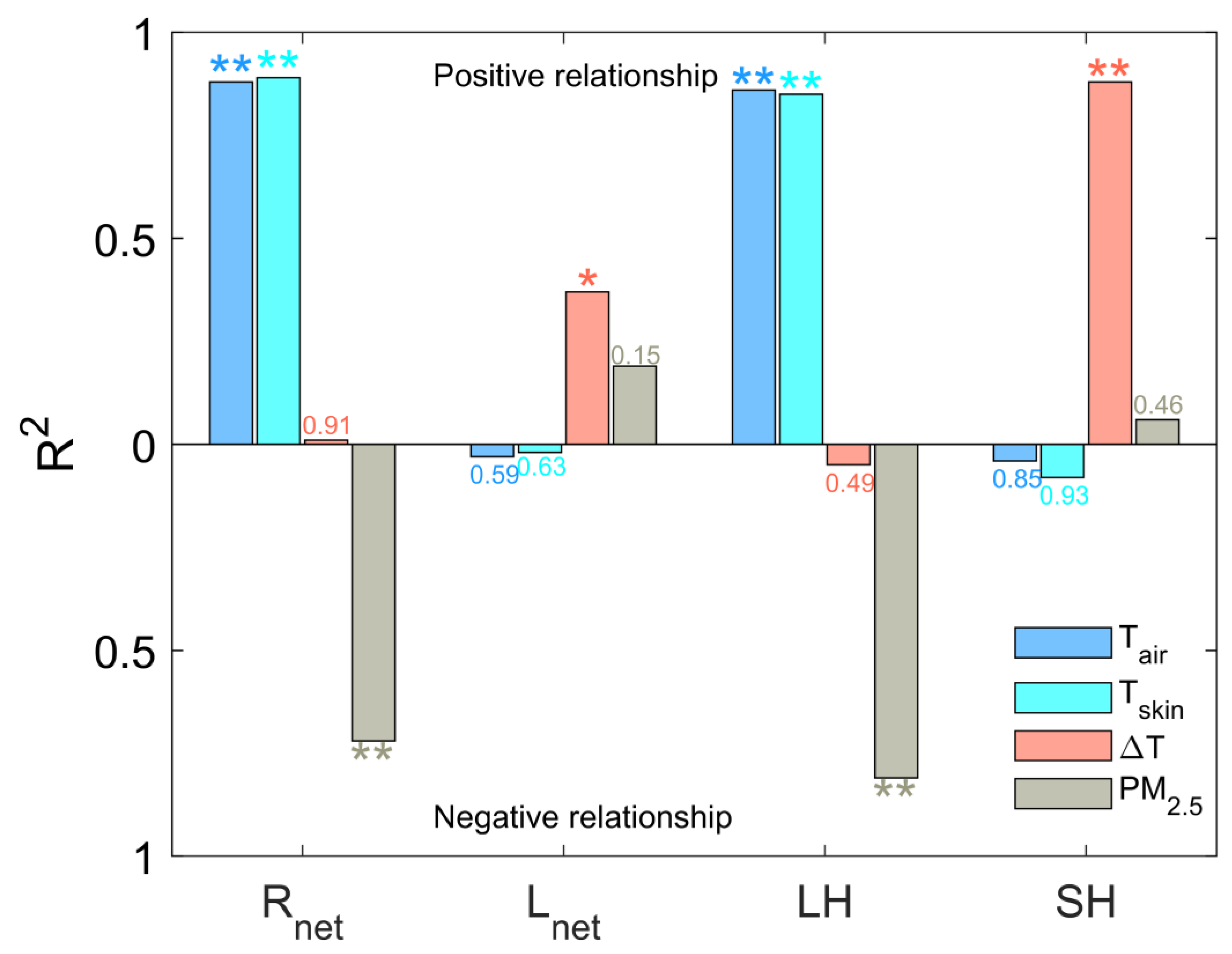
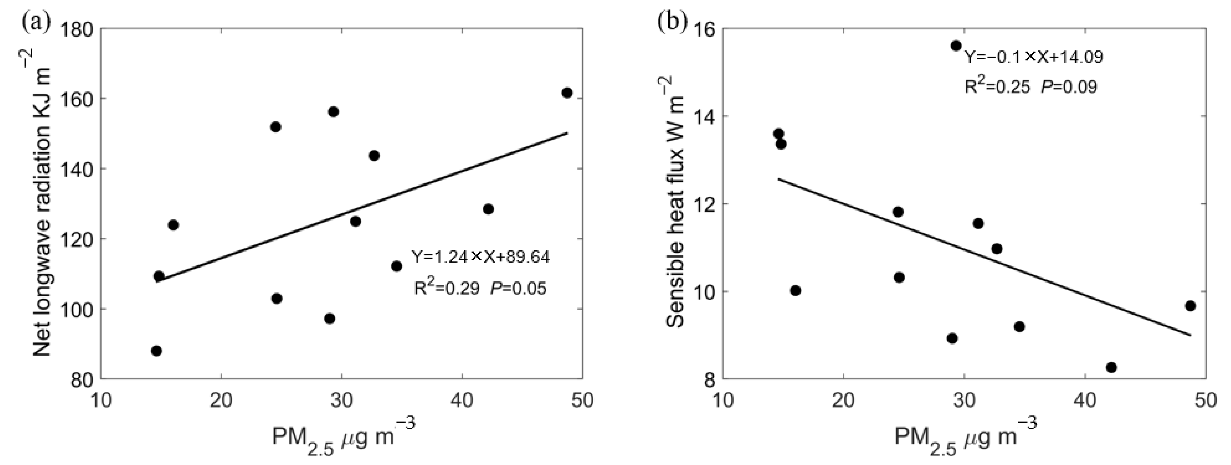
3.3. Mechanistic Analysis

The relationship between PM_2.5 and local surface temperature (T_air and T_skin), along with net shortwave radiation (R_net, downward), net longwave radiation (Lnet, upward), latent heat (LH), and sensible heat (SH) on an annual scale, is depicted in Figure 8. A significant positive correlation was observed between surface temperatures (T_air and T_skin) and R_net (p ≤ 0.001), while no significant relationship (p > 0.5) was found between L_net and temperature. L_net showed an increasing trend, although this trend was not statistically significant (p = 0.15). However, a notable decrease in R_net was associated with increasing PM_2.5 (p ≤ 0.001) on an annual scale, consistent with the findings of Stocker et al. [36]. PM_2.5 reduced the amount of solar radiation reaching the surface through absorption and scattering, resulting in a decrease in both R_net and T_skin. Nevertheless, the relationship between PM_2.5 changed in the same months of adjacent years, and changes in R_net did not show a significant correlation (R² = 0.24, p > 0.5). Research suggests that the absorption of solar radiation by PM_2.5 directly causes an increase in T_air, which in turn enhances downward longwave radiation [23,37,38], which may be explain the significant correlation between the temperature difference and L_net (p ≤ 0.05). Although our research demonstrates the effect of PM_2.5 on R_net and L_net on annual scale, there was still no significant correlation between the effect of PM_2.5 changes on R_net and L_net in the Nanchang region on a seasonal scale. This may be due to the uncertainty over the three years, which could mask the true signals of the changes. Further research is still needed to increase the amount of data.

The energy exchange between the surface and the air is represented by the values of latent heat flux (LH) and sensible heat flux (SH). As shown in Figure 8, there was a significant and positive correlation (p ≤ 0.001) between temperatures and LH (upward), and PM_2.5 had a negative correlation with LH (p ≤ 0.001), suggesting that PM_2.5 regulates changes in surface temperature and air temperature through LH. Studies have shown that PM_2.5 has hygroscopic properties [39,40]. Therefore, under the condition of low wind speed (a mean wind speed of lower than 4 m s⁻¹ at the FA and AX site) in Nanchang, PM_2.5 tended to accumulate, which increased the condensation of water vapor in the air and reduced LH. However, LH did not affect the inversion, as evidenced by their poor relationship (p = 0.49). There was a poor relationship (p > 0.8) between temperature and SH (upward), and the relationship between PM_2.5 and SH was also weak (p = 0.46). However, the linear correlation between SH and surface inversion (ΔT) was highly significant (p ≤ 0.001), and the intensity of the inversion decreased with increasing SH. The difference between T_air and T_skin was one of the main factors driving the SH. However, SH was not significantly correlated with T_air and T_skin, nor with PM_2.5, suggesting that PM_2.5 does not affect SH directly, but rather by changing the difference between T_air and T_skin.

There was a significant positive correlation between PM_2.5 and L_net during the night (p = 0.05) (Figure 9), whereas the correlation between PM_2.5 and L_net during the day was weak (p = 0.26) (Figure A2). During the day, PM_2.5 absorbed solar radiation, which led to an increase in temperature and subsequently the emittance of longwave radiation. Consequently, the impact of PM_2.5 on L_net was modulated. At night, PM_2.5 absorbed the longwave radiation emitted by the surface, and there was a significant linear relationship. Furthermore, as PM_2.5 levels increased at night, T_skin decreased, resulting in a weakening trend of SH (p = 0.09). PM_2.5 was strongly correlated with LH, but its correlation with SH was not significant, and the impact of SH on temperature may also have been insignificant, potentially due to the accumulation of PM_2.5 at the surface. This accumulation could prevent upward longwave radiation, thereby suppressing temperature changes, while LH primarily depends on water vapor transport. When PM_2.5 is higher, LH tends to be smaller [10]. SH and PM_2.5 showed opposite linear relationships during the day and at night. During the day, the ground absorbed solar radiation, causing an increase in T_skin and SH. PM_2.5 significantly affects urban temperature, and the presence and high levels of PM_2.5 absorption components may obscure the ultra-high temperature phenomenon that occurs in urban development [41].

PM_2.5 is indeed transported and dispersed by atmospheric circulation, with the wind field being the most significant factor in reducing PM_2.5 [42]. Absorbing aerosols lower surface temperatures and weaken turbulent exchange; however, they also heat the upper atmosphere, contributing to the formation of inversions [43,44]. Research has also showed that absorbing aerosols can heat the atmosphere, potentially counteracting the impact of reduced surface sensible heat on buoyancy [45,46,47]. Nevertheless, due to data limitations, this study only examined the impact of surface PM_2.5 changes on local surface temperature. It is challenging to isolate the effects of wind fields and topographic factors on local surface temperatures with the limited observations available. Therefore, future research should combine more observations with numerical models to further explore the interaction between PM_2.5 and meteorological factors.

4. Conclusions

The effect of PM_2.5 on local surface temperature was investigated by linear regression and regression analysis using PM_2.5 data from two ground-based monitoring stations in Nanchang City from 2020 to 2022. The results show that the seasonal variation in PM_2.5 in Nanchang is pronounced, being highest in winter and lowest in summer, while PM_2.5 is higher in urban areas than in suburban areas. PM_2.5 can affect the surface temperature, and on an annual scale, the surface temperature in Nanchang decreases with the increase in PM_2.5. PM_2.5 significantly reduces the net shortwave radiation reaching the ground and the latent heat, which in turn affects the surface air temperature and skin temperature, independent of the effects of wind speed and topography. In addition, the skin temperature in Nanchang is lower than the surface air temperature, indicating an inversion. PM_2.5 moderates the temperature decrease by regulating the latent heat flux, while it lowers the surface temperature by absorbing the sensible heat flux and maintaining the surface inversion.

References

1. Jenamani, K.R. Alarming rise in fog and pollution causing a fall in maximum temperature over Delhi. Curr. Sci. 2007, 93, 314–322. Available online: http://www.jstor.org/stable/24099461 (accessed on 2 March 2025).
2. Twomey, S. The influence of pollution on the shortwave albedo of clouds. J. Atmos. Sci. 1977, 34, 1149–1152. [Google Scholar] [CrossRef]
3. Li, H.D.; Sodoudi, S.; Liu, J.F.; Tao, W. Temporal variation of urban aerosol pollution island and its relationship with urban heat island. Atmos. Res. 2020, 241, 104957. [Google Scholar] [CrossRef]
4. Talukdar, S.; Jana, S.; Maitra, A. Dominance of pollutant aerosols over an urban region and its impact on boundary layer temperature profile. J. Geophys. Res. Atmos. 2017, 122, 1001–1014. [Google Scholar] [CrossRef]
5. Lin, Y.L.; Zou, J.L.; Yang, W.; Li, C.-Q. A review of recent advances in research on PM2.5 in China. Int. J. Envion. Res. Public Health 2018, 15, 438. [Google Scholar] [CrossRef]
6. Dai, W.; Gao, J.Q.; Wang, B.; Ouyang, F. Statistical Analysis of Weather Effects on PM2.5. Adv. Mat. Res. 2013, 610–613, 1033–1040. [Google Scholar] [CrossRef]
7. Li, Z.; Chao, C.; Ping, W.; Chen, Z.; Cao, S.; Wang, Q.; Xie, G.; Wan, Y.; Wang, Y.; Lu, B. Influence of atmospheric fine particulate matter (PM2.5) pollution on indoor environment during winter in Beijing. Build. Environ. 2015, 87, 283–291. [Google Scholar] [CrossRef]
8. Megaritis, A.G.; Fountoukis, C.; Charalampidis, P.E.; Denier van der Gon, H.A.C.; Pilinis, C.; Pandis, S.N. Linking climate and air quality over Europe: Effects of meteorology on PM2.5 concentrations. Atmos. Chem. Phys. 2014, 14, 10283–10298. [Google Scholar] [CrossRef]
9. Qu, W.J.; Wang, J.; Zhang, X.Y.; Yang, Z.F.; Gao, S.H. Effect of cold wave on winter visibility over eastern China. J. Geophys. Res. Atmos. 2015, 120, 2394–2406. [Google Scholar] [CrossRef]
10. Chen, D.; Liu, Z.Q.; Fast, J.; Ban, J.M. Simulations of sulfate–nitrate–ammonium (SNA) aerosols during the extreme haze events over northern China in October 2014. Atmos. Chem. Phys. 2016, 16, 10707–10724. [Google Scholar] [CrossRef]
11. Zheng, Z.F.; Xu, G.R.; Li, Q.C.; Chen, C.L.; Li, J.B. Effect of precipitation on reducing atmospheric pollutant over Beijing. Atmos. Pollut. Res. 2019, 10, 1443–1453. [Google Scholar] [CrossRef]
12. Wang, Y.S.; Yao, L.; Wang, L.L.; Liu, Z.R.; Ji, D.S.; Tang, G.Q.; Zhang, J.K.; Sun, Y.; Hu, B.; Xin, J.Y. Mechanism for the formation of the January 2013 heavy haze pollution episode over central and eastern China. Sci. China 2014, 57, 14–25. [Google Scholar] [CrossRef]
13. Li, Z.Q.; Xia, X.G.; Cribb, M.; Mi, W.; Holben, B.; Wang, P.C.; Chen, H.B.; Tsay, S.C.; Eck, T.F.; Zhao, F.S.; et al. Aerosol optical properties and their radiative effects in northern China. J. Geophys. Res. Atmos. 2008, 113, 1–15. [Google Scholar] [CrossRef]
14. Yang, Y.; Chen, M.; Zhao, X.J.; Chen, D.; Fan, S.Y.; Guo, J.P.; Ai, S. Impacts of aerosol–radiation interaction on meteorological forecasts over northern China by offline coupling of the WRF-Chem-simulated aerosol optical depth into WRF: A case study during a heavy pollution event. Atmos. Chem. Phys. 2020, 20, 12527–12547. [Google Scholar] [CrossRef]
15. Zhang, X.Y.; Wang, J.Z.; Wang, Y.Q.; Liu, H.L.; Sun, J.Y.; Zhang, Y.M. Changes in chemical components of aerosol particles in different haze regions in China from 2006 to 2013 and contribution of meteorological factors. Atmos. Chem. Phys. 2015, 15, 12935–12952. [Google Scholar] [CrossRef]
16. Dey, S.; Tripathi, S.N.; Mishra, S.K. Probable mixing state of aerosols in the Indo-Gangetic Basin, northern India. Geophys. Res. Lett. 2008, 35, L03808. [Google Scholar] [CrossRef]
17. Im, U.; Markakis, K.; Koçak, M.; Gerasopoulos, E.; Daskalakis, N.; Mihalopoulos, N.; Poupkou, A.; Kındap, T.; Unal, A.; Kanakidou, M. Summertime aerosol chemical composition in the Eastern Mediterranean and its sensitivity to temperature. Atmos. Environ. 2012, 50, 164–173. [Google Scholar] [CrossRef]
18. Cao, C.; Lee, X.H.; Liu, S.D.; Schultz, N.; Xiao, W.; Zhang, M.; Zhao, L. Urban heat islands in China enhanced by haze pollution. Nat. Commun. 2016, 7, 12509. [Google Scholar] [CrossRef]
19. Wu, H.; Wang, T.J.; Fang, H.; Ma, Y.P.; Han, Y.Q.; Huang, S.; Yao, Y.A.; Shi, J.Q. Impact of aerosol on the urban heat island intensity in Nanjing. Trans. Atmos. Sci. 2014, 37, 425–431. [Google Scholar] [CrossRef]
20. Wu, H.; Wang, T.J.; Riemer, N.; Chen, P.L.; Li, M.M.; Li, S. Urban heat island impacted by fine particles in Nanjing, China. Sci. Rep. 2017, 7, 11422. [Google Scholar] [CrossRef]
21. Barbaro, E.; de Arellano, J.V.G.; Ouwersloot, H.G.; Schröter, J.S.; Donovan, D.P.; Krol, M.C. Aerosols in the convective boundary layer: Shortwave radiation effects on the coupled land-atmosphere system. J. Geophys. Res. Atmos. 2014, 119, 5845–5863. [Google Scholar] [CrossRef]
22. Wang, T.; Wong, C.H.; Cheung, T.F.; Blake, D.R.; Arimoto, R.; Baumann, K.; Tang, J.; Ding, G.A.; Yu, X.M.; Li, Y.S.; et al. Relationships of trace gases and aerosols and the emission characteristics at Lin’an, a rural site in eastern China, during spring 2001. J. Geophys. Res. Atmos. 2004, 109. [Google Scholar] [CrossRef]
23. Wang, L.L.; Gao, Z.Q.; Miao, S.G.; Guo, X.F.; Sun, T.; Liu, M.F.; Li, D. Contrasting characteristics of the surface energy balance between the urban and rural areas of Beijing. Adv. Atmos. Sci. 2015, 32, 505–514. [Google Scholar] [CrossRef]
24. Du, C.; Liu, S.; Yu, X.; Li, X.M.; Chen, C.; Peng, Y.; Dong, Y.; Dong, Z.P.; Wang, F.Q. Urban boundary layer height characteristics and relationship with particulate matter mass concentrations in Xi’an, central China. Aerosol Air Qual. Res. 2013, 13, 1598–1607. [Google Scholar] [CrossRef]
25. Wang, H.; Xue, M.; Zhang, X.Y.; Liu, H.L.; Zhou, C.H.; Tan, S.C.; Che, H.Z.; Chen, B.; Li, T. Mesoscale modeling study of the interactions between aerosols and PBL meteorology during a haze episode in Jing-Jin-Ji (China) and its nearby surrounding region-Part 1: Aerosol distributions and meteorological features. Atmos. Chem. Phys. 2015, 15, 3257–3275. [Google Scholar] [CrossRef]
26. Wu, M.; Wu, D.; Fan, Q.; Wang, B.M.; Li, H.W.; Fan, S.J. Observational studies of the meteorological characteristics associated with poor air quality over the Pearl River Delta in China. Atmos. Chem. Phys. 2013, 13, 10755–10766. [Google Scholar] [CrossRef]
27. Thermo Scientific. TEOM 1405-DF: Dichotomous Ambient Particulate Monitor with FDMS Option; 42-010815 Revision, A.003; Thermo Scientific: Franklin, MA, USA, 2009. [Google Scholar]
28. Hersbach, H.; Bell, B.; Berrisford, P.; Hirahara, S.; Horányi, A.; Muñoz-Sabater, J.; Nicolas, J.; Peubey, C.; Radu, R.; Schepers, D.; et al. The ERA5 global reanalysis. Q. J. R. Meteorol. Soc. 2020, 146, 1999–2049. [Google Scholar] [CrossRef]
29. Bretherton, C.; Widmann, M.; Dymnikov, V.; Wallace, J.; Bladé, I. The effective number of spatial degrees of freedom of a time-varying field. J. Clim. 1999, 12, 1990–2009. [Google Scholar] [CrossRef]
30. Louie, P.K.K.; Chow, J.C.; Chen, L.W.A.; Watson, J.G.; Leung, G.; Sin, D.W.M. PM2.5 chemical composition in Hong Kong: Urban and regional variations. Sci. Total Environ. 2005, 338, 267–281. [Google Scholar] [CrossRef]
31. Zhao, P.S.; Dong, F.; He, D.; Zhao, X.J.; Zhang, X.L.; Zhang, W.Z.; Yao, Q.; Liu, H.Y. Characteristics of concentrations and chemical compositions for PM2.5 in the region of Beijing, Tianjin, and Hebei, China. Atmos. Chem. Phys. 2013, 13, 4631–4644. [Google Scholar] [CrossRef]
32. Zhang, R.; Jing, J.; Tao, J.; Hsu, S.C.; Wang, G.; Cao, J.; Lee, C.S.L.; Zhu, L.; Chen, Z.; Zhao, Y.; et al. Chemical characterization and source apportionment of PM2.5 in Beijing: Seasonal perspective. Atmos. Chem. Phys. 2013, 13, 7053–7074. [Google Scholar] [CrossRef]
33. Liao, H.; Chang, W.; Yang, Y. Climatic effects of air pollutants over China: A review. Adv. Atmos. Sci. 2015, 32, 115–139. [Google Scholar] [CrossRef]
34. Song, Z.J.; Li, R.H.; Qiu, R.Y.; Liu, S.Y.; Tan, C.; Li, Q.P.; Ge, W.; Han, X.J.; Tang, X.G.; Shi, W.Y.; et al. Global land surface temperature influenced by vegetation cover and PM2.5 from 2001 to 2016. Remote Sens. 2018, 10, 2034. [Google Scholar] [CrossRef]
35. Gao, Y.; Zhang, M.; Liu, Z.; Wang, L.; Wang, P.; Xia, X.; Tao, M.; Zhu, L. Modeling the feedback between aerosol and meteorological variables in the atmospheric boundary layer during a severe fog-haze event over the North China Plain. Atmos. Chem. Phys. 2015, 15, 4279–4295. [Google Scholar] [CrossRef]
36. Stocker, T.F.; Qin, D.; Plattner, G.-K.; Tignor, M.M.B.; Allen, S.K.; Boschung, J.; Nauels, A.; Xia, Y.; Bex, V.; Midgley, P.M. (Eds.) Climate Change 2013: The Physical Science Basis; Contribution of Working Group I to the Fifth Assessment Report of IPCC the Intergovernmental Panel on Climate Change; Cambridge University Press: Cambridge, UK, 2014. [Google Scholar] [CrossRef]
37. Jonsson, P.; Eliasson, I.; Holmer, B.; Grimmond, C.S.B. Longwave incoming radiation in the Tropics: Results from field work in three African cities. Theor. Appl. Clim. 2006, 85, 185–201. [Google Scholar] [CrossRef]
38. Dufresne, J.L.; Gautier, C.; Ricchiazzi, P.; Fouquart, Y. Longwave scattering effects of mineral aerosols. J. Atmos. Sci. 2002, 59, 1959–1966. [Google Scholar] [CrossRef]
39. Ding, J.; Dai, Q.L.; Zhang, Y.F.; Xu, J.; Huangfu, Y.Q.; Feng, Y.C. Air humidity affects secondary aerosol formation in different pathways. Sci. Total Environ. 2021, 759, 143540. [Google Scholar] [CrossRef]
40. Kong, L.W.; Hu, M.; Tan, Q.W.; Feng, M.; Qu, Y.; An, J.L.; Zhang, Y.H.; Liu, X.G.; Cheng, N.L.; Deng, Y.J.; et al. Key role of atmospheric water content in the formation of regional haze in Southern China. Atmos. Environ. 2019, 216, 116918. [Google Scholar] [CrossRef]
41. Wu, H.; Wang, T.J.; Wang, Q.G.; Cao, Y.; Qu, Y.W.; Nie, D.Y. Radiative effects and chemical compositions of fine particles modulating urban heat island in Nanjing, China. Atmos. Environ. 2021, 247, 118201. [Google Scholar] [CrossRef]
42. Chan, C.K.; Yao, X. Air pollution in mega cities in China. Atmos. Environ. 2008, 42, 1–42. [Google Scholar] [CrossRef]
43. Johnson, B.T.; Heese, B.; McFarlane, S.A.; Chazette, P.; Jones, A.; Bellouin, N. Vertical distribution and radiative effects of mineral dust and biomass burning aerosol over West Africa during DABEX. J. Geophys. Res. Atmos. 2008, 113, 1–16. [Google Scholar] [CrossRef]
44. Malavelle, F.; Pont, V.; Mallet, M.; Solmon, F.; Johnson, B.; Leon, J.F.; Liousse, C. Simulation of aerosol radiative effects over West Africa during DABEX and AMMA SOP-0. J. Geophys. Res. Atmos. 2011, 116. [Google Scholar] [CrossRef]
45. Barbaro, E.; de Arellano, J.V.G.; Krol, M.C.; Holtslag, A.A.M. Impacts of aerosol shortwave radiation absorption on the dynamics of an idealized convective atmospheric boundary layer. Bound. Layer Meteorol. 2013, 148, 31–49. [Google Scholar] [CrossRef]
46. Sun, T.; Che, H.; Qi, B.; Wang, Y.Q.; Dong, Y.S.; Xia, X.G.; Wang, H.; Gui, K.; Zheng, Y.; Zhao, H.J.; et al. Characterization of vertical distribution and radiative forcing of ambient aerosol over the Yangtze River Delta during 2013–2015. Sci. Total Environ. 2019, 650, 1846–1857. [Google Scholar] [CrossRef]
47. Yu, H.; Liu, S.C.; Dickinson, R.E. Radiative effects of aerosols on the evolution of the atmospheric boundary layer. J. Geophys. Res. Atmos 2002, 107, AAC 3-1–AAC 3-14. [Google Scholar] [CrossRef]
Figure 1. Location of Nanchang City in mainland China and its PM2.5 monitoring sites (a), together with the vicinity of Jiangxi Forestry Academy Station FA (b) and Aixi Lake Station AX (c).
Atmosphere 16 00411 g001
Figure 2. PM2.5 measured at the FA (a,b) and AX (c,d) sites, respectively. Letters (a,c) are the original data in FA and AX, while (b,d) are the data after quality control at each site.
Atmosphere 16 00411 g002
Figure 3. Seasonal variations in surface PM2.5 concentration and surface temperature at FA (a) and AX (b). The columns represent the mean concentration of PM2.5, while the red lines with circles indicate the air temperature for various years, and the black lines with markers denote the skin temperature.
Atmosphere 16 00411 g003
Figure 4. The inter-annual differences and the corresponding temperature differences of PM2.5 at FA (a) and AX (b) during the same season. The stripes represent the differences in PM2.5, the brown dot represents the differences in surface air temperature (Tair), and the black dots represent the differences in skin temperature (Tskin). Superscript 1 indicates the difference between 2021 and 2020, and superscript 2 represents the difference between 2022 and 2021.
Atmosphere 16 00411 g004
Figure 5. Relationship between PM2.5 and temperature. (a) Mean values for 2020–2022, air temperature (b) and skin temperature (c) vs. PM2.5 in FA, and (d,e) air temperature and skin temperature vs. PM2.5 in AX.
Atmosphere 16 00411 g005
Figure 6. The relationship between monthly temperature difference and PM2.5 at (a) FA and (b) AX, and (c) the average.
Atmosphere 16 00411 g006
Figure 7. Relationship between temperature difference and PM2.5 under non-inversion (a,b) and inversion (c,d). Letters (a,c) represent FA, while (c,d) represent AX.
Atmosphere 16 00411 g007
Figure 8. Relationship between PM2.5 and local surface temperature (Tair and Tskin) with net shortwave radiation (Rnet, downward), net longwave radiation (Lnet, upward), latent heat (LH), and sensible heat (SH) on an annual scale. ΔT, Tskin minus Tair. The positive correlation is depicted in the top panel, while the negative correlation is shown in the bottom panel. The values adjacent to the columns represent the confidence level (p-value); * signifies p ≤ 0.05 and ** signifies p ≤ 0.001.
Atmosphere 16 00411 g008
Figure 9. The impact of PM2.5 on net longwave radiation (a) and sensible heat (b) during nighttime.
Atmosphere 16 00411 g009
Disclaimer/Publisher’s Note: The statements, opinions and data contained in all publications are solely those of the individual author(s) and contributor(s) and not of MDPI and/or the editor(s). MDPI and/or the editor(s) disclaim responsibility for any injury to people or property resulting from any ideas, methods, instructions or products referred to in the content.