Urban Air Pollution in the Global South: A Never-Ending Crisis?

Abstract

Among the challenges the human population needs to address are threats of global pandemics, increasing socioeconomic inequality, especially in developing countries, and anthropogenic climate change. The latter’s effect has been amplified with the arrival of 2023/24 El Niño, causing an exceptional drought in the Amazon basin, significantly affecting fire conditions and hydroelectric power production in several South American countries, including Ecuador. This study analyzes five criteria pollutants—carbon monoxide (CO), nitrogen dioxide (NO₂), sulfur dioxide (SO₂), ozone (O₃), and particulate matter ≤ 2.5 µm (PM_2.5)—during 2019–2024 in Quito, Ecuador, a high-elevation tropical metropolis. Despite long-term efforts to regulate emissions, air pollution levels continue to rise, driven by overlapping crises, including energy shortages, political unrest, and extreme weather events. The persistent failure to improve air quality underscores the vulnerability of developing nations to climate change-induced energy instability and the urgent need for adaptive, diversified, and resilient future energy planning. Without immediate shifts in climate adaptation policies, cities like Quito will continue to experience worsening air quality, with severe implications for public health and environmental sustainability.

1. Introduction

Urban air pollution is affected by various factors, including energy production, transportation systems, public health crises, socio-political events or conflicts, meteorological conditions, urban infrastructure, and population density [1]. These elements interact dynamically, leading to spatial and temporal variations in air quality with significant implications for public health and environmental sustainability [2]. Fossil fuel combustion remains the primary cause of air pollution, particularly in regions with lower fuel standards and high-sulfur-content fuels [3]. Energy and heat production are among the largest global contributors to atmospheric pollution [4], reinforcing the urgency of transitioning to cleaner energy sources such as hydroelectricity. As electricity demand rises, power generation must adapt to local climate conditions. However, hydropower’s dependence on water availability makes it increasingly vulnerable to climate variability, including droughts and extreme weather events [5].

Consequently, amidst all the global challenges, such as environmental pollution [6], overpopulation [7], urbanization [8], the COVID-19 pandemic [9,10], and socioeconomic inequality leading to political unrest [11], the ongoing climate crisis remains a dominant force. Known for numerous negative effects across all the regions of the world, human-induced climate change has also triggered an unprecedented drought in the Amazon River Basin since mid-2023 [12], worsened by the 2023/24 El Niño phenomenon (i.e., low rainfall and higher-than-normal temperatures). As a result, the World Meteorological Organization (WMO) confirmed that 2023 and 2024 were the two warmest years on record [13,14]. Record-low Amazon river levels have disrupted communities, ecosystems, and transportation and severely impacted regional hydroelectric power production [15]. Given that a significant share of electricity in this part of the world is derived from hydropower—Brazil (80%), Colombia (79%), Venezuela (68%), Ecuador (65%), Peru (55%), and Bolivia (32%)—this led to power shortages starting in June 2023 [12,16,17]. Consequently, reliance on fossil-fuel-based backup thermoelectric plants and diesel generators has created unforeseen emissions of combustion-related pollutants that are being released into the urban atmosphere [18,19,20].

Anthropogenic activities responsible for greenhouse gas emissions and climate change also contribute to toxic air pollution, endangering environmental and human health. According to the World Health Organization (WHO), air pollution is linked to seven million premature deaths annually, with 89% occurring in low- and middle-income countries, where air quality regulations are often less stringent [21,22,23,24]. Thus, many regulations have been applied to reduce air pollution levels and guarantee a healthy environment for human populations. Success stories are vast, showing the impact of regulations and technological improvements resulting in the continuous reduction in pollution levels in Australia [25], EU [23,24,26,27], USA [28,29], and even recently in China [30]. Moreover, in the very recent past, during the COVID-19 pandemic, the world experienced an experimental halt to air pollution due to seized anthropogenic activity [9]. However, despite a good promise of learning from the COVID-19 pandemic and improving global air quality [25], most of the countries saw a rebound back to “normal” air pollution levels right away [9,31].

While developed countries strictly safeguard air quality and uphold the right to a healthy environment, developing nations face complex challenges where unforeseen natural and anthropogenic crises can abruptly worsen urban air pollution. Though numerous studies have documented air pollution trends in developed and developing countries [27,28,32,33], there is a notable scarcity of longitudinal research in small and mid-size cities of the Global South [34]. Gaps in air quality data hamper a comprehensive understanding of air quality dynamics in these regions [35,36]. Inspired by the “Air Quality Stripes” project [37], this study aims to provide a perspective on air pollution variability in Quito, Ecuador, an unlisted city in global air quality assessments. We analyze trends over the past six years (i.e., pre-pandemic—post-pandemic), focusing on historical and seasonal fluctuations in pollutant concentrations, linking observed rises and falls to their potential drivers. As a high-elevation tropical metropolis, Quito experiences frequent and unpredictable air quality fluctuations, exacerbated by energy crises, socio-political instability, and economic constraints. This study seeks to capture the multifaceted and dynamic nature of air pollution in Quito, emphasizing the interplay of diesel-based power generation, civil protests, and pandemic-related mobility shifts. We analyze the behavior of five key criteria pollutants—carbon monoxide (CO), nitrogen dioxide (NO₂), sulfur dioxide (SO₂), ozone (O₃), and fine particulate matter (PM_2.5) (aerodynamic diameter ≤ 2.5 µm)—to illustrate how pollution patterns evolve under constant socio-environmental turbulence. This work contributes to a broader understanding of pollution dynamics in rapidly urbanizing, politically volatile, and climate-sensitive regions by presenting a comprehensive temporal assessment of air quality trends.

2. Materials and Methods

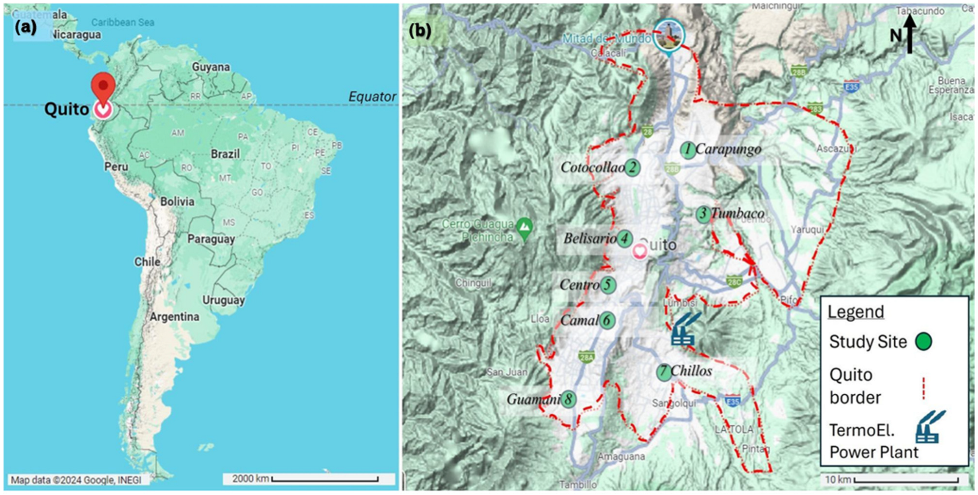
2.1. Study Site

As a pioneering UNESCO cultural heritage site, Quito, Ecuador (Figure 1a) holds the title of being the world’s highest constitutional capital, with an average elevation of 2850 m above sea level (m.a.s.l.) [38]. The city’s metropolitan district spans a diverse elevation range from 500 to 4500 m.a.s.l., extending approximately 34.8 km north–south and 13.5 km east–west. Administratively, it is divided into 55 units, comprising 32 urban and 33 rural sectors [39]. Experiencing a rapid expansion, the district covers 4218 km² and is home to over 2.7 million residents, catching up with Ecuador’s largest city—the coastal hub of Guayaquil [40] (Figure 1b).

Quito faces persistent air quality challenges, primarily due to reduced oxygen availability at high altitude (around 70% of sea-level levels), reliance on low-quality fuels, outdated combustion technologies, and limited urban infrastructure constrained by mountainous terrain. Additional factors common in developing cities, such as chaotic traffic patterns and inadequate vehicle maintenance, further exacerbate the issue [22,41].

Despite these challenges, Quito benefits from a mild, spring-like climate, with two distinct seasons: a wet period (September to May) and a dry season (June to August) [41]. Strong solar irradiance during the morning hours rapidly breaks up the frequent nocturnal temperature inversion, facilitating natural ventilation and dispersing pollutants from this high-altitude metropolis.

For this study, data from eight study sites, representing different districts of Quito, were investigated: (1) Carapungo (2660 m.a.s.l., coord. 78°26′50″ W, 0°5′54″ S); (2) Cotocollao (2739 m.a.s.l., coord. 78°29′50″ W, 0°6′28″ S); (3) Tumbaco (2355 m.a.s.l., coord. 78°24′12.4164″ W, 0°12′53.334″ S); (4) Belisario (2835 m.a.s.l., coord. 78°29′24″ W, 0°10′48″ S); (5) Centro (2820 m.a.s.l., coord. 78°30′36″ W, 0°13′12″ S); (6) Camal (2840 m.a.s.l., coord. 78°30′36″ W, 0°15′00″ S); (7) Chillos (2453 m.a.s.l., coord. 78°27′36″ W, 0°18′00″ S); and (8) Guamani (3066 m.a.s.l., coord. 78°33′5″ W, 0°19′51″ S) (Figure 1b).

2.2. Pollution Data Collection and Analysis

Since 2004, the Secretariat of Environment under Quito’s municipal administration has overseen the city’s air quality monitoring network. The system continuously measures key atmospheric pollutants—CO, NO₂, SO₂, O₃, and PM_2.5—using U.S. Environmental Protection Agency (EPA)-approved instruments installed on municipal building rooftops, following EPA protocols. Detailed descriptions of the methodology can be found in previous studies [9,41,42,43,44].

For carbon monoxide (CO) monitoring, the Thermo Fisher Scientific 48i analyzer (EPA No. RFCA-0981-054) is utilized (Thermo Fisher Scientific, Franklin, MA, USA). This non-dispersive infrared (NDIR) sensor detects CO levels by analyzing infrared light absorption, ensuring continuous data collection with periodic calibration for accuracy [42]. Nitrogen oxides (NO_x) are quantified using the Thermo Fisher 42i chemiluminescence analyzer (EPA No. RFNA-1289-074) (Thermo Fisher Scientific, Franklin, MA, USA). This instrument measures nitric oxide (NO) concentration based on its reaction with ozone, producing light emissions proportional to NO concentration. The system logs data continuously, with regular calibration maintaining measurement precision [42]. For sulfur dioxide (SO₂) analysis, a Thermo Fisher Scientific 43i pulsed fluorescence analyzer (EPA No. EQSA-0486-060) is employed (Thermo Fisher Scientific, Franklin, MA, USA). The device exposes SO₂ molecules to ultraviolet (UV) light, inducing fluorescence, the intensity of which correlates with the SO₂ concentration. Automated calibration ensures high measurement reliability [42]. Ozone (O₃) levels are tracked using a UV photometric analyzer (Thermo Fisher 49i; EPA No. EQOA-0880-047) (Thermo Fisher Scientific, Franklin, MA, USA). The system determines ozone concentration by measuring the degree of UV light absorption by O₃ molecules. The instrument logs measurements continuously to maintain data integrity and undergoes periodic calibration [42]. Measurements of fine particulate matter (PM_2.5) rely on a Beta Attenuation Monitor (BAM; Thermo Scientific FH62C14-DHS 5014i, EPA No. EQPM-0609-183) (Thermo Fisher Scientific, Franklin, MA, USA). This technique involves directing beta radiation through collected particulate matter on a filter tape, where attenuation levels correspond to the mass concentration of airborne particles. Data are recorded hourly, with automated QA/QC protocols ensuring measurement precision [42].

The collected air quality data are automatically stored in the Secretariat of Environment’s public repository, available for download at https://datosambiente.quito.gob.ec/ (accessed on 10 January 2025).

Hourly data for criteria pollutants (CO, NO₂, SO₂, O_3, and PM_2.5) were obtained from 1 January 2019 to 31 December 2024. This six-year period includes two events of political protests (i.e., 2–13 October 2019 and 13–30 June 2022), an extremely strict period of COVID-19 restrictions’ (i.e., 16 March–31 May 2020) followed by a progressive relaxation period (i.e., 1 June–1 July 2020), and three separate episodes of electrical crises: (i) Episode#1: 2–4 h/day blackouts on 27 October–2 December 2023; (ii) Episode#2: with 4–8 h/day blackouts in 16–30 April 2024; and (iii) Episode#3 with 7–14 h/day blackouts 23 September–22 December 2024). The study period included a close-by volcano eruption (i.e., 21 October–22 December 2022). To examine temporal trends, hourly pollutant data were processed to calculate the following: (i) diurnal trends by averaging concentrations over each 24 h period across the study period; (ii) monthly 24 h trends to assess seasonal and interannual variations over the six years; and (iii) monthly and yearly averages to identify long-term trends.

As different districts of Quito had a complex rotating blackout schedule throughout the study period, the data were averaged over all eight study sites. However, once some districts lose power supply, the others function normally, meaning it is not a total but partial city blackout.

Further data exploration focused on a paired t-test to evaluate if there were significant differences in air pollutant concentrations between different years (2019–2024). Then, from the “Data” tab, “Data Analysis ToolPak” was activated, and the “t-Test” was selected. After setting the significance level to 0.05, the analysis was carried out.

The analysis figure creation was performed using Microsoft Excel, MS PowerPoint, and IGOR-Pro 6, Wavemetrics software.

To obtain meteorological data for eight sites, complete weather stations MetOne with automatic sensors were used (Met One Instruments Inc., Grants Pass, OR, USA), also managed by the Secretariat of Environment, DMQ. Hourly data for the study period were processed to achieve monthly and yearly averages to smooth out the trends using IGOR-Pro 6 Software.

2.3. Temporal and Spatial Data Analysis

To investigate the temporal and spatial variability of air pollutant concentrations in Quito from 2019 to 2024, boxplots and annulus plots were generated using R v4.3.2 [45] after additional data cleaning, where outliers above the 99.9th percentile were removed to ensure data reliability [19]. Boxplots, created with the ggplot2 [46] and dplyr [47] packages, visualized the yearly distributions of PM_2.5, SO₂, NO₂, O₃, and CO concentrations (PM₁₀ were excluded due to their limited availability) at each monitoring station, displaying the median, interquartile range (IQR), and outliers for each year, with 24 h maximum (red) and average (blue) concentrations annotated above and below each boxplot, respectively, and years with no data marked as “nd” (no data). Annulus plots, generated with the openair package [48,49], overlaid polar annulus markers on a map of Quito (using OpenStreetMap), with concentric rings depicting average pollutant concentrations by wind direction (0° to 360°, north at 0°) and hour of the day (00:00 to 23:00), aggregated by year, and with color intensity indicating concentration levels, enabling the identification of dominant pollution sources and diurnal patterns at each station.

3. Results and Discussion

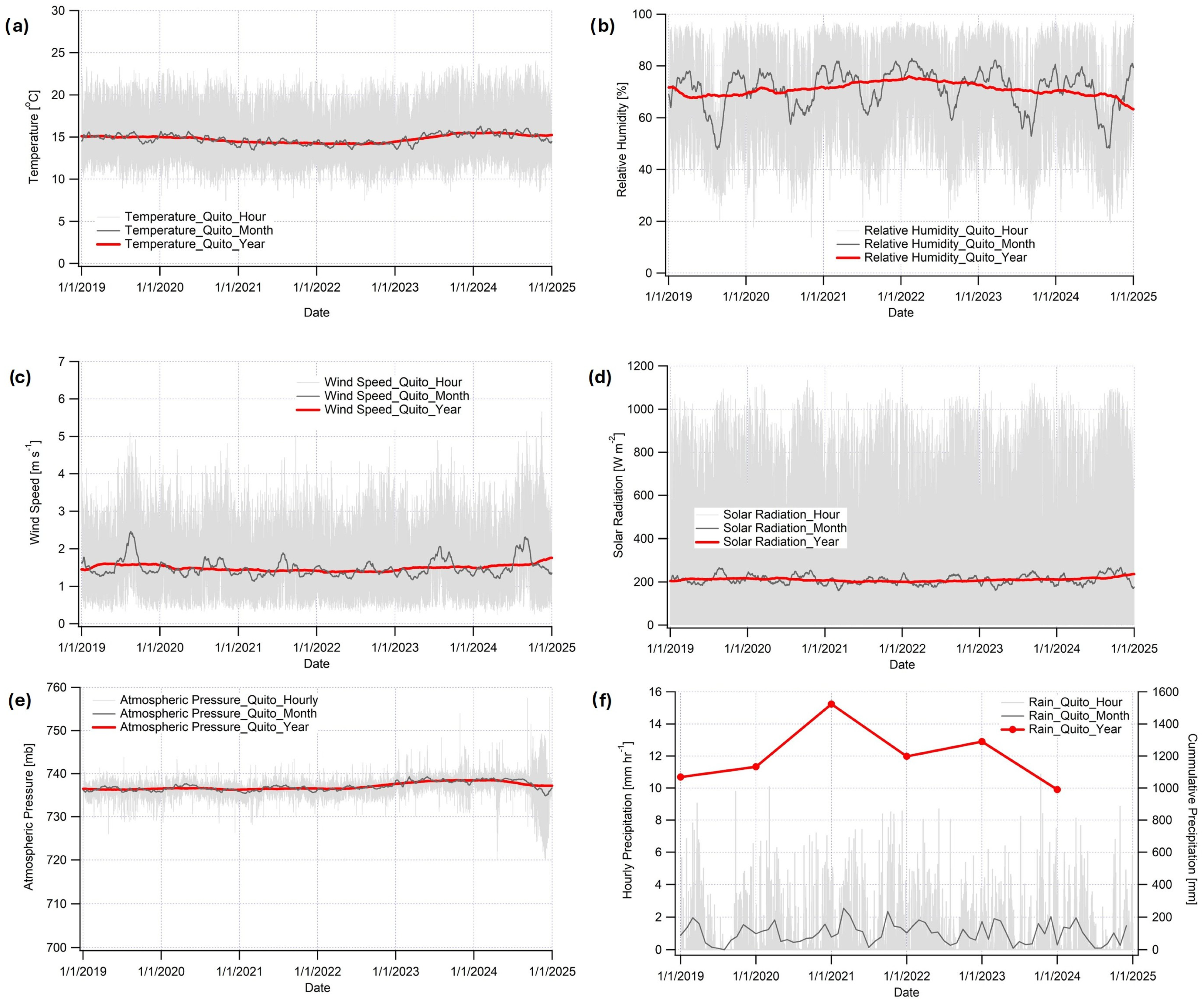
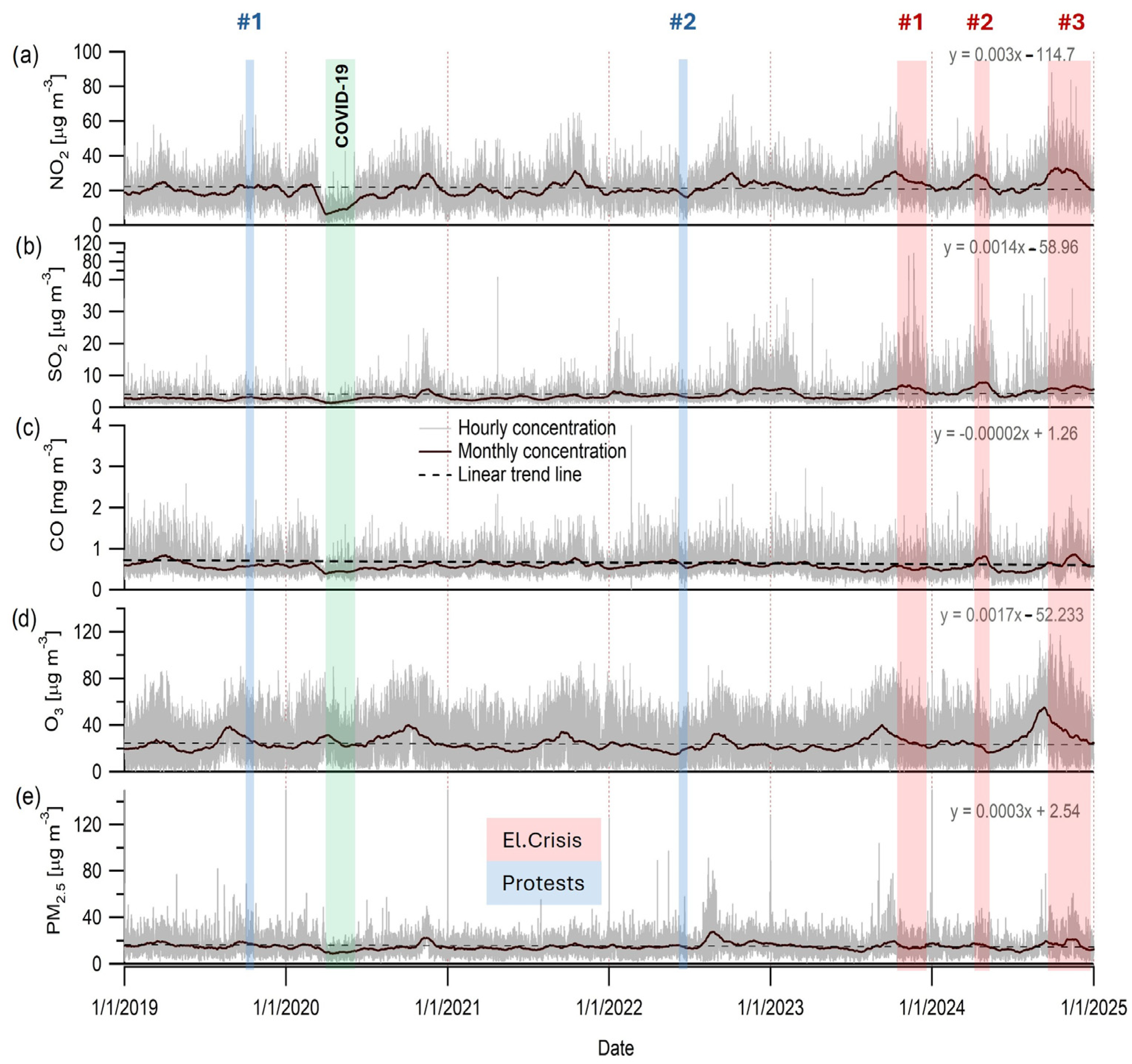
3.1. Time Series of Air Pollution 2019–2024

The study period represents a particularly turbulent time in the recent air quality history of this rapidly growing South American capital. Though weather may impact the air quality, a quick time series review of meteorological parameters showed little variation during the study period (Figure A1, Appendix A). Figure 2 shows that, within a span of six years, Quito experienced two nationwide political protests (i.e., #1: 2–13 October 2019; and #2: 13–30 June 2022), a strict COVID-19 pandemic lockdown (i.e., 16 March–31 May 2020), and three episodes of electricity crises (i.e., Episode #1: 27 October–2 December 2023; Episode #2: 16–30 April 2024; and Episode #3: 23 September–22 December 2024). This period also coincided with severe wildfires within the city limits due to a strong El Niño-related drought (i.e., lower than ‘normal’ relative humidity and higher than ‘normal’ temperatures and wind speed) in mid-August to early September 2023 and on 24–25 September 2024, which likely contributed to elevated PM_2.5 and CO levels, as biomass burning added to the pollution burden during the third episode of the electrical crisis.

Overall, the concentrations of four out of five studied criteria air pollutants in Quito indicate an increasing trend over time (2019–2024). The most pronounced increase is observed for NO₂ (Figure 2a), followed by O₃ (Figure 2d), SO₂ (Figure 2b), and PM_2.5 (Figure 2e). This trend is not surprising, as all four pollutants show a clear rise in the past two years, possibly somewhat due to warmer and drier weather conditions and more likely due to the increased use of additional emission sources, particularly diesel generators [18,19]. It can be deduced that the pollution peaks appear during the specific events of electricity crises. For instance, during the September–December 2024 crisis, NO₂ hourly concentrations averaged over the whole city peaked at approximately 80 µg/m³ (Figure 2a), while O₃ peaked up to 120 µg/m³ (Figure 2d). Moreover, during Electricity Crises #1 and #2, but not #3, all-city hourly average levels for SO₂ reached as high as 100 µg/m³ (Figure 2b), suggesting that the pollution levels could be even higher in some districts. We note that during Electrical Crisis #3, blackouts lasted up to 14 h, causing emergency batteries at multiple monitoring sites to fail, resulting in gaps in air quality data. Consequently, actual pollutant concentrations were likely significantly higher than reported. Future studies could apply advanced estimation methods to better assess the true air quality levels that the population was exposed to during the last three months of 2024. Additionally, the long-term health impacts of prolonged exposure to unreported toxic pollution and noise warrant further investigation through epidemiological studies once health data become available from Ecuador’s Ministry of Health.

While PM_2.5 (Figure 2e) does not show an increase due to protests or crises, except during Electricity Crisis #3, its hourly concentrations surge every January 01, varying at around 120–140 µg/m³, reflecting the acute impact of fireworks on the air quality. In addition, PM_2.5 shows an increase, similar to all other pollutants, in the late summer months of August and September, when the city tends to have events of wildfires at the end of dry season. These dry spells during mid-August-early September of 2023 and 2024 were amplified by a record-breaking drought in 2023–2024, which reduced hydropower availability and fueled both electrical shortages and wildfires, intensifying pollutant emissions in the latter half of the study period.

Although CO concentrations exhibit small peaks during the last two crisis events (Figure 2c), they still show an overall decline throughout the study period. It may be explained by the fact that most backup generators operate on diesel, and their contribution to CO emissions is not significant enough to reverse the long-term downward trend due to other causes (i.e., newer technologies and fuel improvements, among others). It is well established that diesel engines are not major emitters of CO [50]. Nevertheless, the CO peaks during the 2024 crises (1 mg/m³) may reflect contributions from wildfire smoke or incomplete combustion in older generators, warranting further investigation. However, a comparative study by May et al. [50] found that diesel engines emit significantly higher levels of NO_x and PM, which helps explain the pronounced increase in NO₂ concentrations.

Finally, amidst these various pollution events, Quito experienced a strict COVID-19 lockdown from 16 March to 31 May 2020. During this period, a significant reduction in all pollutants was observed except for O₃, a trend consistent with evidence from worldwide research. A rapid rebound in air pollution levels followed as human activities resumed. This trend is particularly evident in the NO₂ profile (Figure 2a).

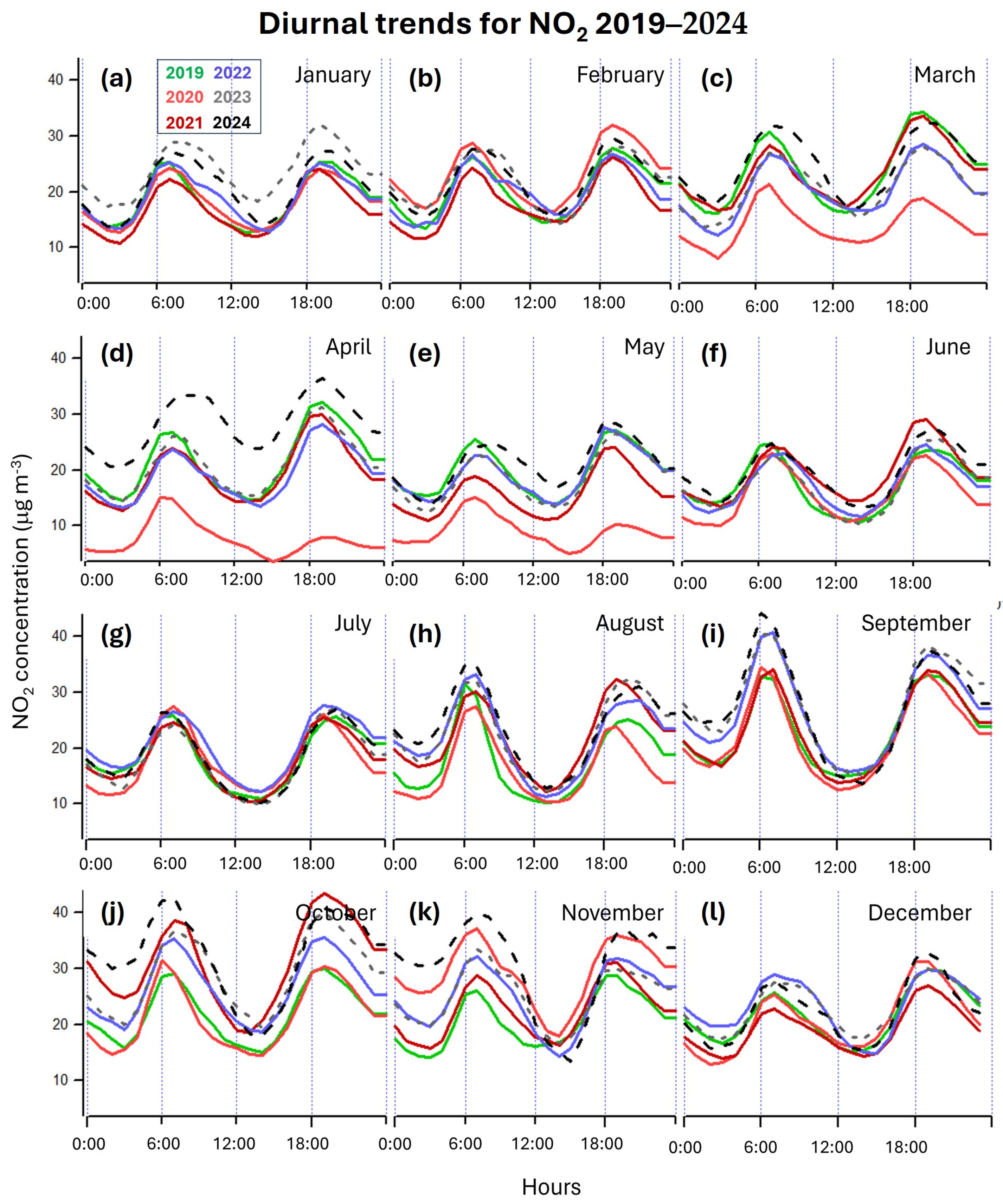
3.2. Diurnal Trends for Each Month of 2019–2024

While most developed countries seem to improve urban air quality over time, in the previous subchapter, we identified that concentrations of four out of the five studied criteria pollutants increased in the recent post-pandemic period. To better identify the reasons or “breaking points” in these trends, the data are further represented as diurnal trends in a comparative manner for each studied year.

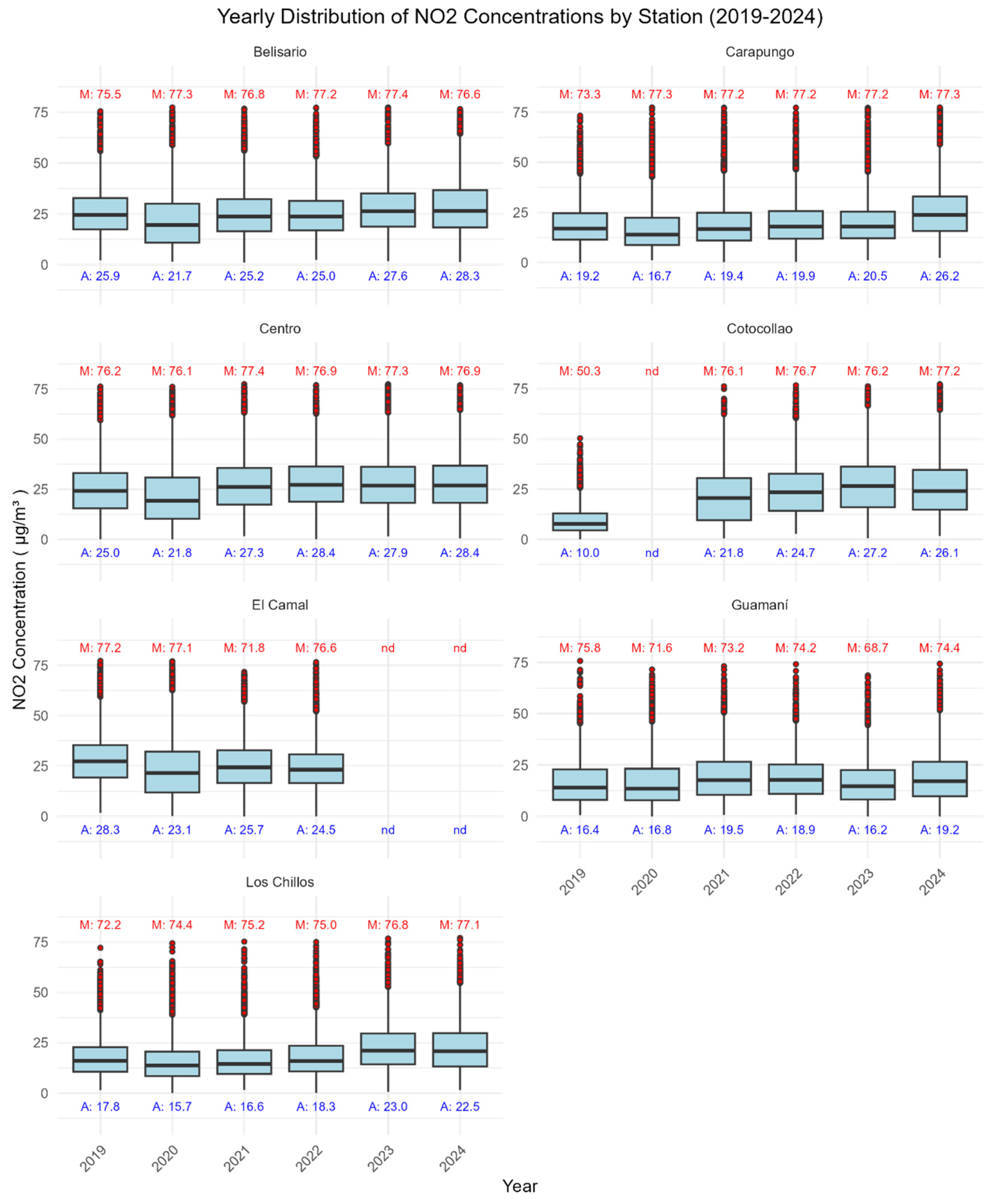
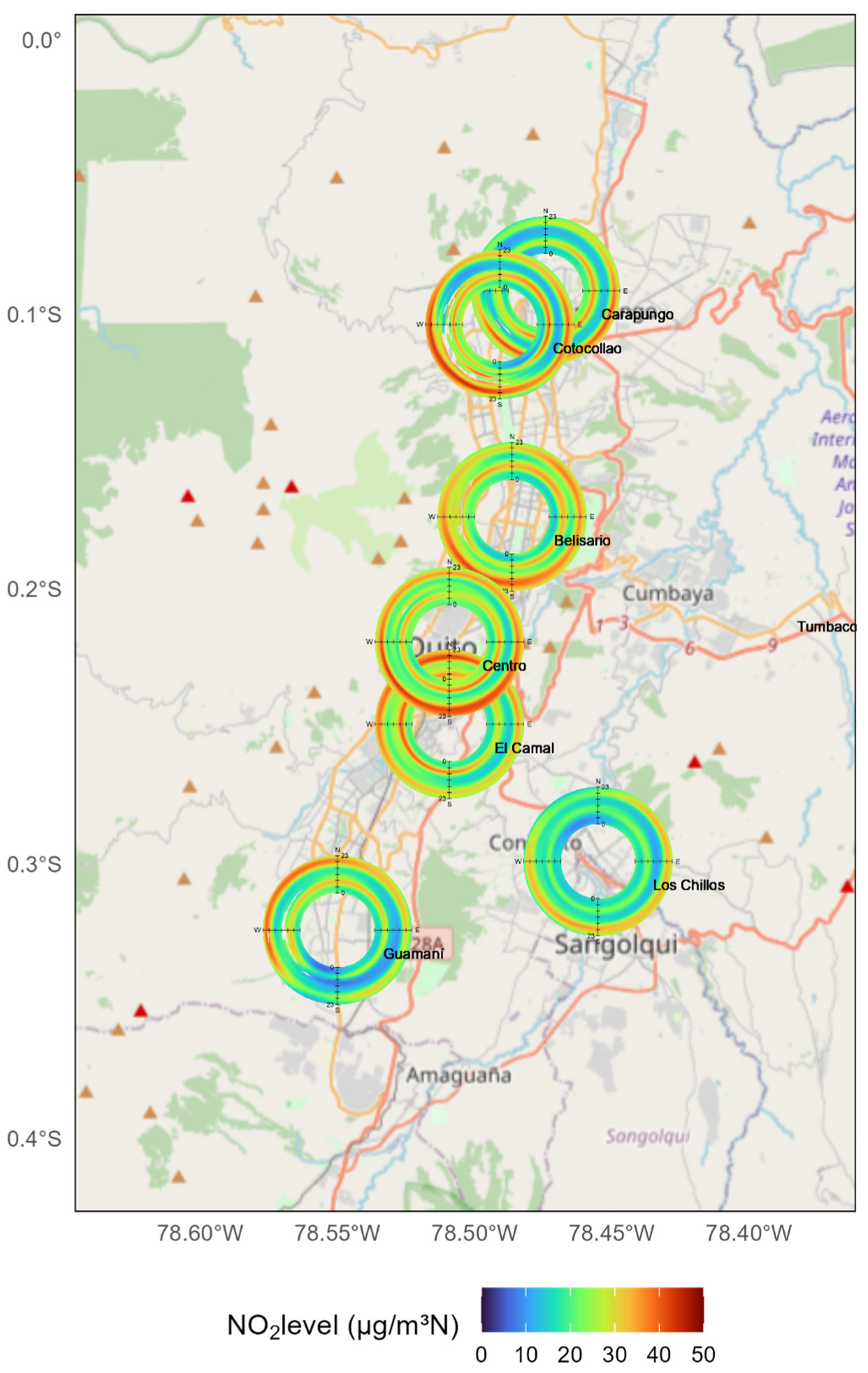
3.2.1. NO₂ Diurnal Trends

Figure 2a shows that NO₂ exhibits the greatest increasing trend over the past six years. Figure 3 illustrates the diurnal trends of NO₂ concentrations for each month across the study period (2019–2024). The first general observation is that, in nearly all months, the diurnal trends of each preceding year display lower values than the subsequent year, except for March−May 2019 (Figure 3c–e), where NO₂ levels are elevated, resembling those observed in 2024.

The impact of COVID-19 pandemic restrictions is visible from March (Figure 3c) to May (Figure 3e) 2020, showing significant change in diurnal trends (p < 0.05, Figure A2, Appendix A). Even though some circulation restrictions remained in place for the next three months, the NO₂ trends quickly returned to ‘normal’ during June–August (Figure 3h), 2020. Moreover, by September 2020 (Figure 3i), pollution patterns had returned to a “business-as-usual” state, and by November 2020 (Figure 3k), NO₂ levels had increased even further, suggesting a possible “compensatory” effect as anthropogenic activities rebounded after the pandemic-induced slowdown.

Regarding the influence of political protests, reduced NO₂ concentrations were observed in October 2019 (Figure 3j), with a significant difference in diurnal trends from other years (p < 0.05, Figure A2, Appendix A). This confirms previous findings, where a 30% reduction in NO₂ concentrations during the national protests was reported for the whole city [51].

Finally, the energy crises—particularly those of 2024—seem to have caused the most substantial NO₂ increases with significant changes in diurnal trends, especially in April 2024 (Figure 3d) and during the September–November 2024 period (Figure 3i–k and Figure A2, Appendix A). During the electricity crises in 2024, blackouts lasting up to 14 h per day led to particularly high NO₂ concentrations, even during nighttime hours (Figure 3d,j–k). As a perfective, it is unrealistic to expect air quality improvements through urban fleet electrification when the existing electricity supply is insufficient to meet basic household demand. Without a substantial increase in clean energy production, the shift to electric vehicles could inadvertently lead to higher emissions, as increased reliance on thermoelectric power generation—often fueled by fossil sources—would significantly elevate pollutant levels.

Additionally, due to the extreme drought associated with the 2023/24 El Niño phase [12], multiple wildfires occurred near the city, likely contributing to increased combustion-related gas and particle pollution in August–September 2023 and 2024 (Figure 3h,i). However, NO₂ concentrations were also elevated in late summer 2022, likely due to similar wildfire activity in the region. The diurnal trends of these unusual months are significantly different from 2019—the ‘business-as-usual period’ (Figure A2, Appendix A). These findings might suggest the ‘new reality’ regarding increasing global temperatures and other climate change factors causing more beneficial conditions for wildfires in the region. The health implications must be considered.

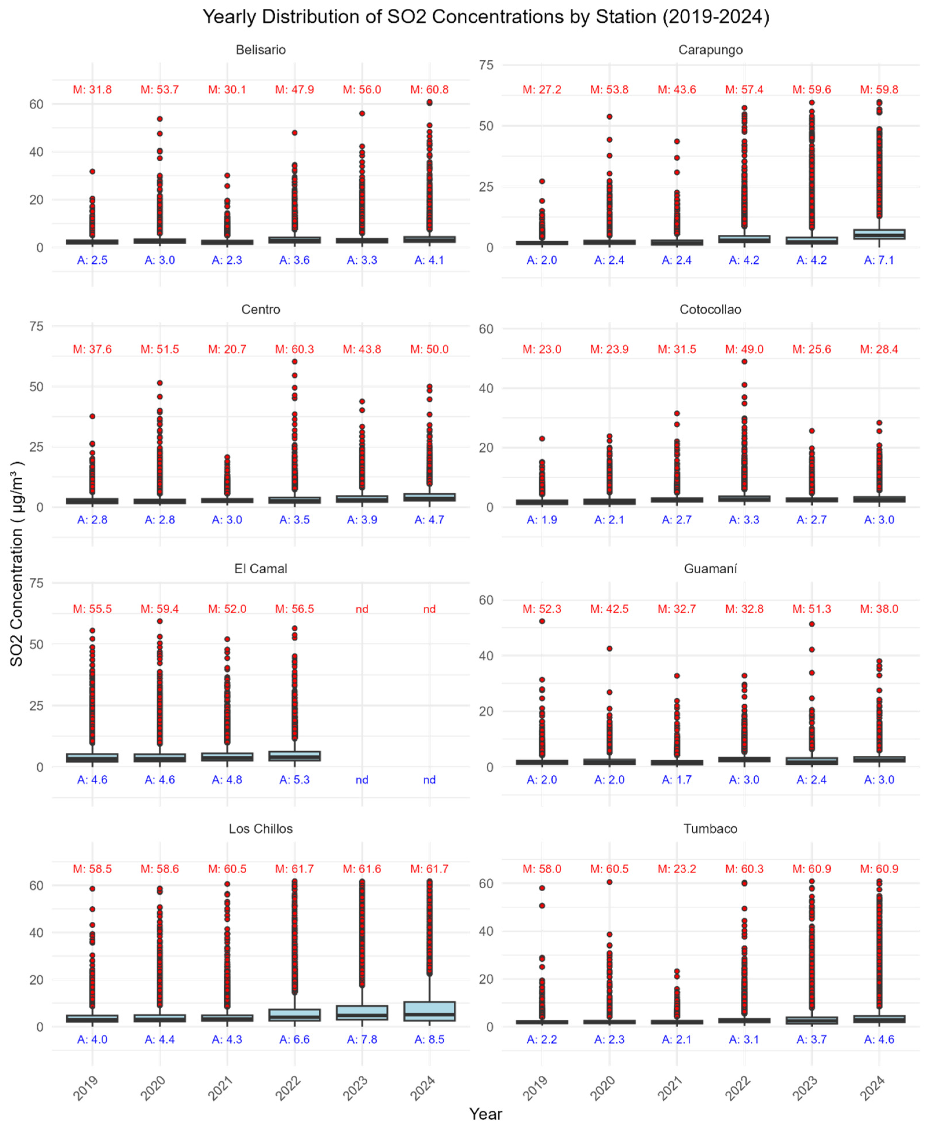
3.2.2. SO₂ Diurnal Trends

As shown in Figure 2b, SO₂ concentrations exhibit an increasing trend throughout the study period, further evident in the month-to-month analysis (Figure 4). Notably, SO₂ levels have generally risen over the past three years. Although the energy crisis began in late 2023, we observed an increase in SO₂ concentrations as early as 2022, including during months without blackouts (i.e., January, February, and May; see Figure 4a,b,e). It may be attributed to rising electricity demand, which was met by fossil fuel-powered local thermoelectric plants [52].

Except for June, SO₂ trends during 2019–2021 significantly differ from 2022–2024 for most months of the year (Figure A2, Appendix A). Even at a glance, it is evident that what were once distinct morning rush hour peaks have become more prolonged. The pattern suggests the emergence of new pollution sources, most likely related to thermoelectric power generation. Additionally, SO₂ levels appear to be higher during electricity crisis periods (i.e., April, 2024, and October–December, 2023 and 2024; see Figure 4d,j–l). Thus, the trend in this pollutant serves as a clear example of the following: (i) inadequate energy planning and (ii) how climate change impacts renewable energy production—both of which significantly affect air quality in urban areas of developing countries.

Furthermore, regarding SO₂ diurnal trends, the typical morning rush hour peaks shift to later hours during blackout periods, likely due to scheduled power outages (Figure 4a–e,j–l). While SO₂ concentrations did not exceed health standards, they exhibited the most pronounced increase from ‘business-as-usual’ levels. Our findings align with previous studies [18,19]. Additionally, there was a clear decline in SO₂ concentrations during the first three months of the COVID-19 pandemic (Figure 4c–e), followed by a slight “compensatory” increase once circulation restrictions were fully lifted (Figure 4k).

Additionally, we note that a nearby Cotopaxi volcano eruption started in late October and went on till December, with volcanic ash from the volcano falling on most districts of Quito starting at 03:30 on 26 November 2022, following a tremor and gas-and-ash emission detected by local seismic stations. Elevated SO₂ trends were registered during November and December of 2022, as this pollutant is commonly emitted during volcanic eruptions.

Additionally, we note that a nearby Cotopaxi volcano eruption began in late October and continued until late December. Volcanic ash reached most districts of Quito starting at 03:30 on 26 November 2022, following a tremor and gas-and-ash emission detected by local seismic stations [53]. Elevated SO₂ concentrations were recorded in November and December 2022 (Figure 4k,l), as this pollutant is commonly emitted during volcanic eruptions, especially common in Ecuador, with a few actively erupting volcanoes.

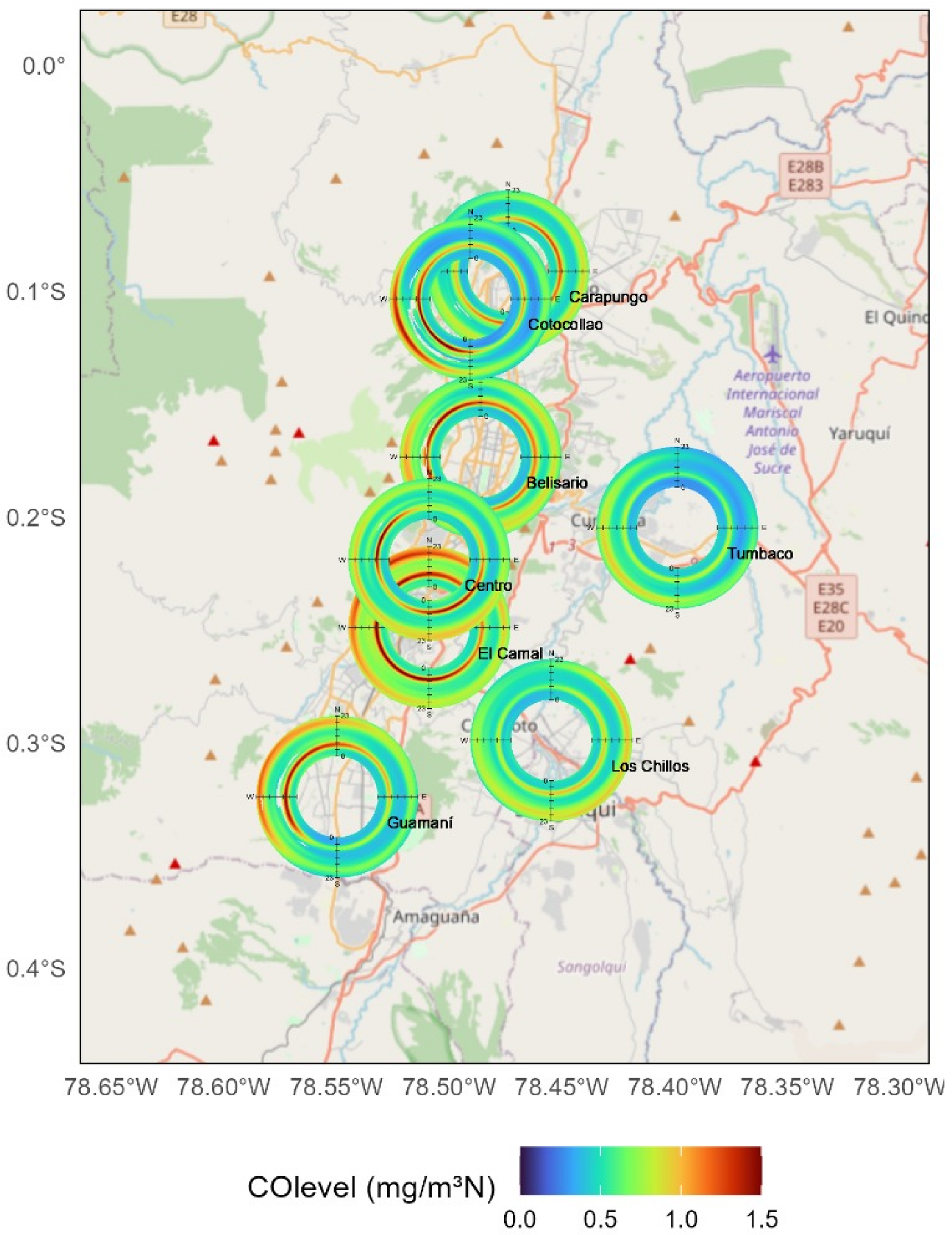
3.2.3. CO Diurnal Trends

Figure 5 presents the diurnal trends of CO concentrations for each month over the six-year study period (2019–2024). As observed for other pollutants, the impact of COVID-19 pandemic restrictions is evident from March (Figure 5c) to May (Figure 5e), 2020.

As reported in Figure 2c, CO is the only one of the five studied pollutants to exhibit a decreasing trend over the last six years. During the later electricity crises (Episodes #2 and #3), CO levels increased, likely due to a surge in the use of smaller, gasoline-powered personal generators, as many residents either purchased or rented them to cope with prolonged blackouts. The city’s streets were filled with the sound of generators and the smell of gasoline. Notably, CO exhibited elevated nighttime concentrations in November 2024. Given that CO is a long-lived pollutant with an atmospheric lifetime of approximately one month, its cumulative buildup over an extended period likely became more pronounced at night. During the daytime, however, concentrations were somewhat diluted due to the deepening of the planetary boundary layer, a common effect in this equatorial city where the solar angle remains high year-round [54].

Across the study period, diurnal CO trends showed little significant difference (Figure A2, Appendix A), except for the clear differences between ‘business-as-usual’ conditions in 2019 and the COVID-19 restriction period (Figure 5d,e), as well as between the electricity crisis months and the corresponding months of relatively stable years such as 2021 and 2022 (i.e., October−November, see Figure 5j,k and Figure A2, Appendix A).

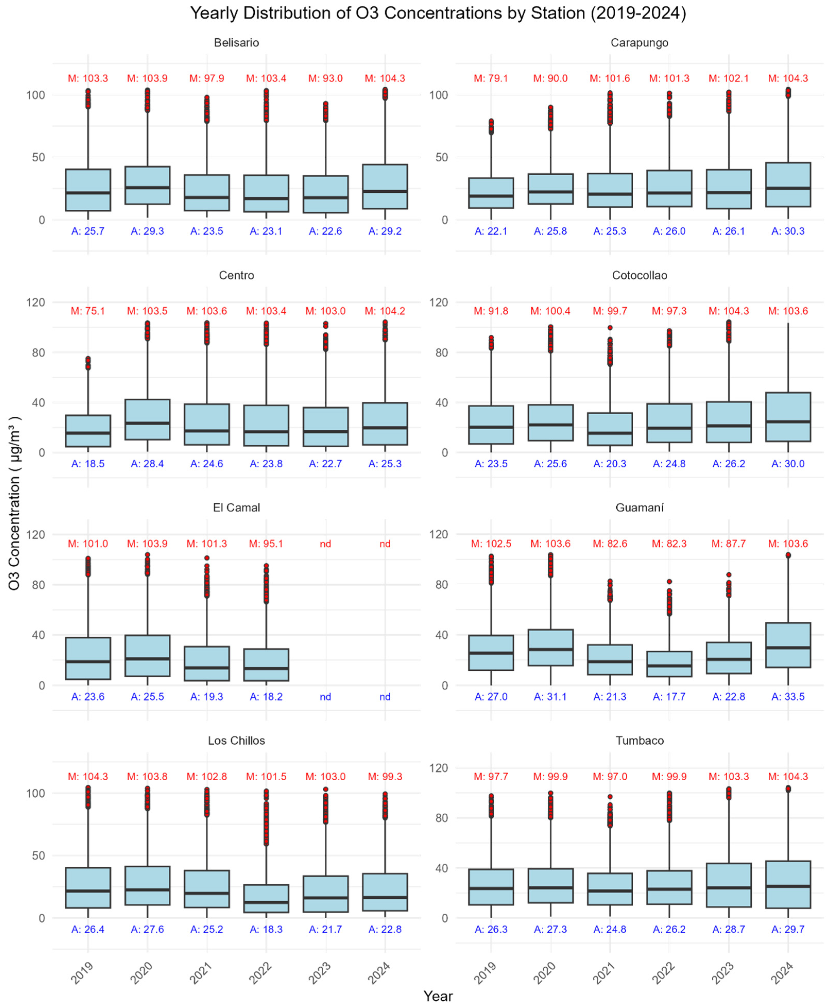
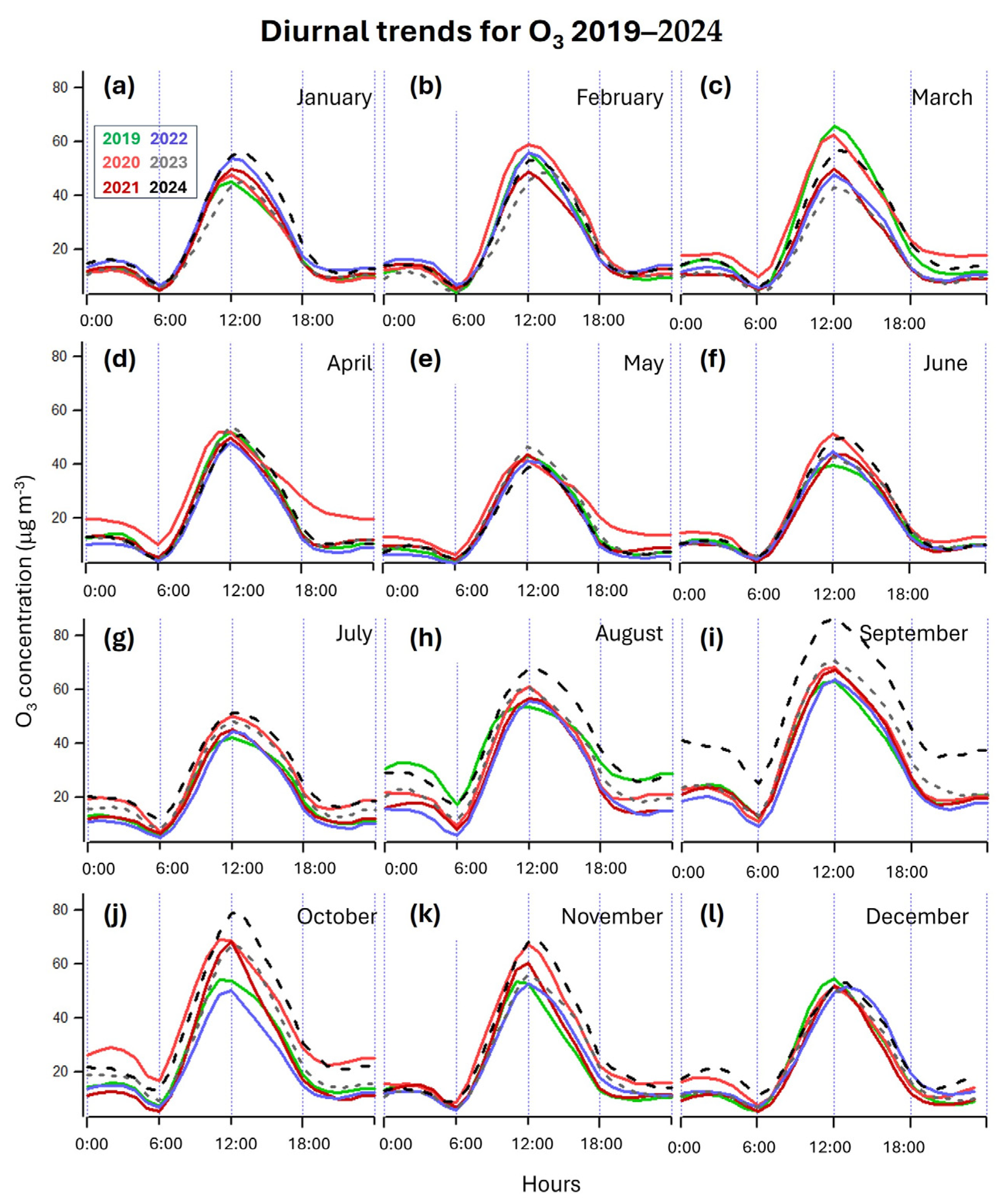
3.2.4. O₃ Diurnal Trends

While some variation in O₃ levels is observed, an overall increasing trend over the study period is evident in Figure 2d and further confirmed by Figure 6. This pollutant exhibits the most significant shift in diurnal concentration patterns for all months of 2023 and 2024 compared to the previous four years (Figure A2, Appendix A). This shift may be attributed to the formation of El Niño, which brings warmer and drier conditions to the region, affecting O₃ concentrations.

In general, the months of August to October consistently show higher O₃ concentrations, likely due to the seasonal coincidence of multiple factors: (i) the dry season (which was particularly severe during the 2023/2024 El Niño event), reducing pollutant removal via wet deposition (Figure A1, Appendix A); and (ii) high solar radiation during this period, which enhances photochemical O₃ formation. This combination of meteorological and anthropogenic factors creates optimal conditions for elevated O₃ levels, though remaining below air quality health standards.

During the second half of 2024 (Figure 6g–k), a period marked by severe electricity shortages, O₃ levels reached their highest recorded concentrations in the study period. It coincided with El Niño-driven drought conditions and high solar radiation, which amplified O₃ production while reducing atmospheric cleansing due to low precipitation.

As expected, O₃ concentrations increased during the COVID-19 lockdown period, a trend widely reported in air quality studies [9]. This phenomenon is attributed to the nonlinear photochemistry of O₃, where a reduction in NO emissions from traffic led to less O₃ destruction via NO titration, allowing O₃ levels to rise.

Additionally, local fires in August may have contributed to further O₃ formation, as biomass burning releases volatile organic compounds (VOCs) that act as O₃ precursors. This suggests that during extreme events such as droughts or energy crises, multiple anthropogenic and natural emission sources interact in complex ways, shaping urban air pollution patterns.

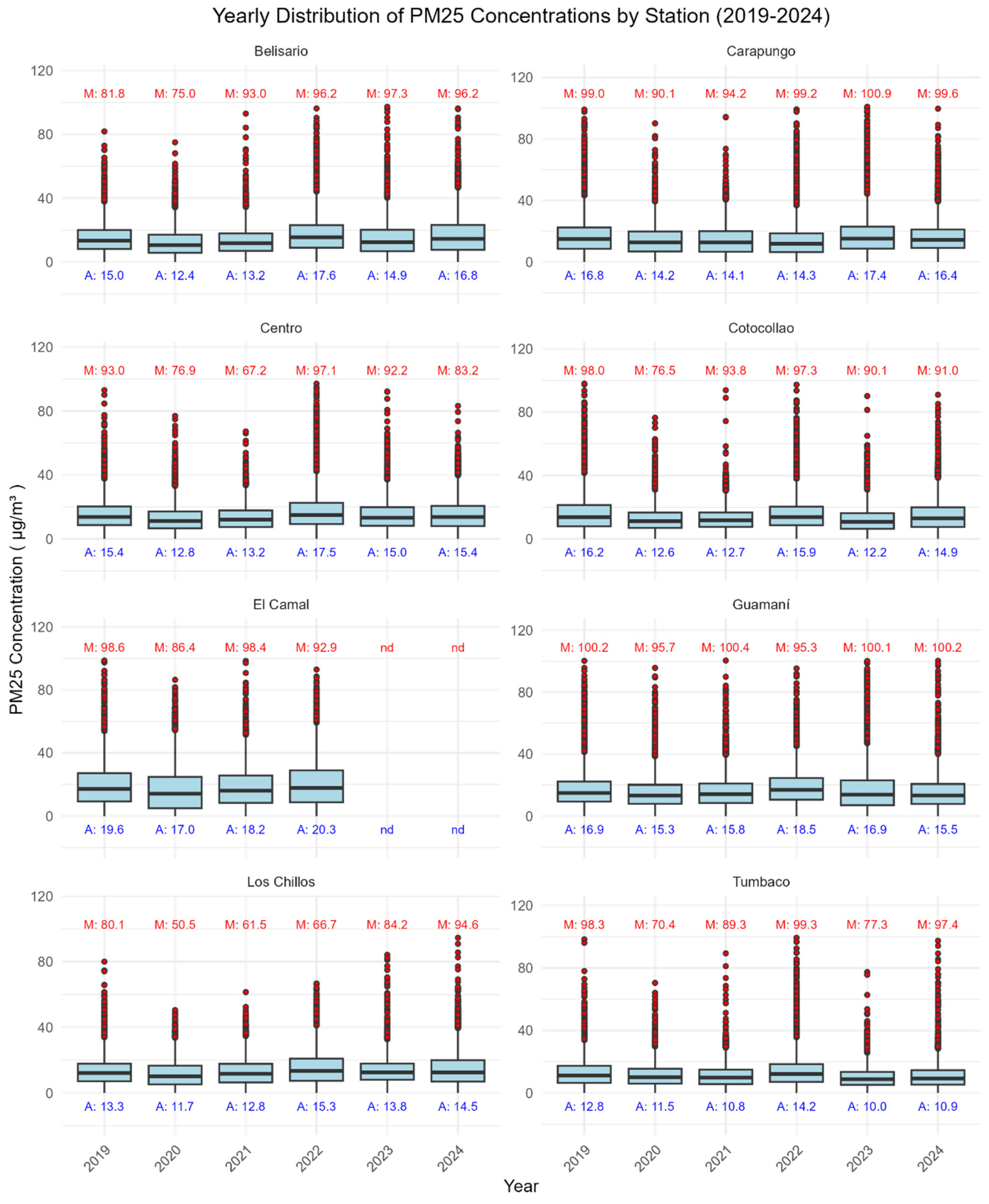
3.2.5. PM_2.5 Diurnal Trends

Figure 7 presents the diurnal trends of PM_2.5 concentrations during the study period (2019–2024). While PM_2.5 levels exhibit a slight overall increase over the last six years, there is distinct competition between 2019 and 2023/2024 in terms of peaks of diurnal trends. It is plausible that, in the absence of the electricity crises, PM_2.5 concentrations would have decreased. However, poor energy management in the country and increased thermoelectric power production within the city likely contributed to elevated PM_2.5 levels in recent years. The long-term trajectory of air quality remains uncertain, but these crises highlight the fragility of air pollution mitigation efforts when confronted with climate change-induced droughts that disrupt hydroelectric power generation. It underscores the necessity of diversifying renewable energy sources to enhance climate resilience and ensure a sustainable energy supply.

A particularly striking anomaly in PM_2.5 levels is observed in August 2022 (Figure 7h). Extensive data validation confirmed that this was not an equipment malfunction or error. Rather, all monitoring sites in Quito recorded a consistent PM_2.5 increase between 11:00 and 17:00 throughout most of August 2022. While periodic air quality deterioration is common in Quito, this pollution level was exceptional. The analysis revealed that this period coincided with extensive wildfires in the Brazilian Amazon [55], likely transporting particulate pollution to the region.

Additionally, local fires further contributed to deteriorating air quality, with some events impacting pollution levels during the daytime and overnight [56]. Similar conditions were observed during the fire seasons of 2023 and 2024; however, fire suppression efforts in those years were more effective, preventing the extreme pollution levels recorded in 2022. August 2022 significantly differs in diurnal trends from any other year, indicating anomalous atmospheric and pollution conditions (Figure A2, Appendix A).

During the first electricity crisis episode (October–December 2023), a reduction in PM_2.5 concentrations was observed, likely due to decreased circulation and economic activity, as some businesses ceased operations during power outages. However, during the more severe electricity crises of 2024, PM_2.5 levels were significantly elevated, with April 2024 (Episode #2, Figure 7d) and November 2024 (Episode #3, Figure 7k) exhibiting distinct diurnal trends compared to previous years (Figure A2, Appendix A). It can likely be attributed to an increased reliance on backup diesel and gasoline generators and the intensified operation of thermoelectric power plants to compensate for hydropower shortages. Importantly, power outages were not uniformly applied across all districts; some areas continued to function while others experienced rotating blackouts due to the outdated thermoelectric power infrastructure’s inability to sustain the full electricity demand. It should also be noted that the actual pollution levels may have been even higher than reported, as many monitoring stations experienced shutdowns due to battery failures during extended 14 h blackouts.

A clear reduction in PM_2.5 concentrations is observed during the COVID-19 lockdown period, particularly in April–May 2020 (Figure 7d,e). These months show significantly different diurnal trends than any other year, reflecting substantial shifts in anthropogenic behavior due to strict mobility restrictions.

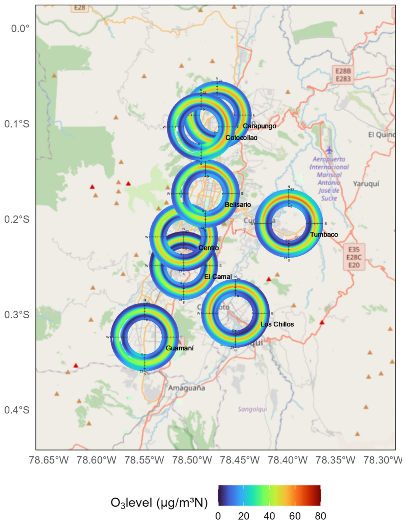
3.3. Spatio-Temporal Analysis

Finally, the spatial and temporal distribution of pollutants in Quito was analyzed to estimate the changes over the study period in each of the eight districts of the air quality network, revealing large variability in air pollutant concentrations across Quito from 2019 to 2024 (

Table 1. Percent change for all studied pollutants (i.e., NO₂, SO₂, CO, O₃, and PM_2.5) for all study sites (with available data) between 2019 and 2024. ND indicates that there were no data during the last two years of this study (e.g., Camal) as the electrical crises affected the equipment function; or a specific pollutant is not measured in this study site, due to economic limitations (e.g., suburban districts of Tumbaco and Chillos).

Site	NO2	SO2	CO	O3	PM2.5
(1) Carapungo	36.46	255.00	20.00	37.10	−2.38
(2) Cotocollao	161.00	57.89	−33.33	27.66	−8.02
(3) Tumbaco	ND	109.09	ND	12.93	−14.84
(4) Belisario	9.27	64.00	33.33	13.62	12.00
(5) Centro	13.60	67.86	−14.29	36.76	0.00
(6) Camal	ND	ND	ND	ND	ND
(7) Chillos	26.40	112.50	ND	−13.64	9.02
(8) Guamani	17.07	50.00	20.00	24.07	−8.28

, Figure A3, Figure A4, Figure A5, Figure A6, Figure A7, Figure A8, Figure A9, Figure A10, Figure A11 and Figure A12, Appendix A). NO₂ levels, exceeding WHO standards (i.e., annual concentration < 10 µg m⁻³), increased in all districts, suggesting consistent increasing fossil fuel combustion emissions in this city (Table 1, Figure A3, Appendix A). Conversely, in residential and commercial zones like Centro, Carapungo, and Belisario, NO₂ showed a consistent upward trend throughout the study period, driven by persistent vehicular traffic, with temporary reductions during the COVID-19 lockdown in 2020, followed by a rebound as mobility restrictions eased. On the other hand, the interquartile ranges (IQR) for SO₂ and O₃ widen in 2024, indicating greater variability during the years with electricity crises, with maxima exceeding 50 µg m⁻³ and 100 µg m⁻³, respectively, in almost all the sites (Table 1, Figure A4 and Figure A6, Appendix A). SO₂ trends in mixed residential–commercial areas like Centro and Carapungo showed more variable profiles, with SO₂ increasing during electricity crises periods due to generator use. Conversely, CO exhibits a variable trend, with concentrations increasing in most sites over the study period (Table 1, Figure A5, Appendix A). This is consistent with reduced emissions from newer technologies and improving fuel quality [22], though minor peaks during the 2024 crises suggest localized gasoline generator use. Highly variable overall trends are recorded for PM_2.5 (Table 1), which exceed health standards (i.e., 5 µg m⁻³) in all city districts, while PM_2.5 showed reductions during the 2020 lockdown, likely due to decreased local activity, though it rose again in 2024 with extended power blackouts. Notably, concentrations in Chillos show a marked increase in 2023–2024, with levels rising, likely reflecting intensified thermoelectric production during the El Niño drought (Figure 2b and Figure A7, Appendix A). These observations highlight the influence of episodic events on pollutant dynamics, necessitating targeted mitigation strategies.

Similarly, the annulus plots provide a detailed spatial analysis of air pollutant concentrations in Quito from 2019 to 2024, complementing the temporal insights offered from box plots by illustrating how pollution levels vary across different districts. These visualizations reveal distinct spatial patterns, with elevated concentrations of NO₂, CO, and PM_2.5 during rush hours in central districts such as El Camal, Centro, and Belisario—likely driven by traffic activity, wildfire smoke, and localized generator use during the 2023–2024 crises (Figure A8, Figure A10 and Figure A12, Appendix A). High levels often align with the orientation of the city’s main highways, suggesting windborne pollution transport from more polluted areas. The suburban district of Los Chillos and the adjacent El Camal show increased SO₂ levels (Figure A9, Appendix A), likely linked to anthropogenic sources such as emissions from the nearby thermoelectric power plant (Figure 1b). Lastly, ozone concentrations peak during midday hours and correlate with easterly winds at urban sites, indicating the transport of biogenic volatile organic compounds (VOCs) from surrounding natural areas. The directional dependency of pollutant concentrations, aligned with wind patterns, underscores the influence of local sources and urban layout, offering critical insights into spatial disparities that support the need for tailored mitigation strategies across Quito’s diverse districts.

The findings of this study highlight temporal and spatial differences in pollution patterns across the metropolis of the Global South, shaped by local sources, geography, and urban infrastructure. It also exposes the fragility of air quality monitoring in times of crisis, where technical and financial limitations can leave communities without critical data. More broadly, this study reflects the volatility of air quality in the developing world, where climate change, power shortages, political instability, and health emergencies collide like waves rocking an already unsteady boat. In this context, air quality becomes a moving target—highly sensitive to external shocks and often hardest to manage where resources are limited. Building resilience in monitoring and policy is essential to protect public health and secure the basic right to clean air for all.

4. Conclusions

This study illustrates the dynamic and unpredictable nature of air pollution in a rapidly growing, high-elevation metropolis, shaped by a mix of climate variability, socio-political instability, and energy challenges. While developing countries struggle to improve air quality, new stressors—many linked to climate change—are shifting the baseline, often reversing past progress. Extreme climate events, such as prolonged droughts and intensified wildfires, are becoming more frequent, adding new sources of air pollution that further burden urban environments. Meanwhile, reliance on outdated and polluting energy solutions during electricity crises exposes structural weaknesses in energy planning, making pollution spikes an unavoidable consequence of poor resilience. Political protests, frequent in developing nations, also disrupt urban air quality in unpredictable ways, either by reducing emissions through mobility restrictions or worsening pollution through fires and traffic congestion. The COVID-19 pandemic offered a brief window of reduced emissions, yet post-lockdown, pollution levels rebounded quickly, if not worsened, showing that no structural improvements were made to sustain cleaner air. This cycle of temporary progress and sudden regression highlights the ongoing failure to adapt air quality management to modern challenges.

The findings reveal a critical challenge for urban air quality management in the Global South: the compounding effects of climate-driven and socio-political stressors create a volatile pollution landscape that demands adaptive strategies. The dramatic increases in pollutants like SO₂, with rises as high as 255% in some districts, underscore the environmental cost of relying on fossil fuel-based energy solutions during crises, such as the 2023–2024 electricity shortages, while natural events like the 2022 Cotopaxi eruption further exacerbate these trends. Similarly, the widespread increase in NO₂, reaching 161% in certain areas, highlights the persistent dominance of traffic-related emissions, amplified by social unrest and post-lockdown rebounds, with only temporary reprieves during events like the 2020 lockdown. These trends, coupled with the variable behavior of PM_2.5—three-fold exceeding WHO standards across all districts despite reductions in some suburban areas—illustrate how local emission sources and external shocks create significant spatial disparities in air quality. The rise in O₃, with increases up to 37.1%, driven by El Niño-related dry conditions, further signals the growing influence of climate change on photochemical pollution. Even CO, which generally declined due to technological improvements, saw localized increases during the 2024 crises, reflecting the unintended consequences of emergency measures like generator use.

Traditional approaches focused on emissions control alone are insufficient when new, climate-driven, and socio-political disruptions constantly reshape pollution patterns. Instead, policies must be tailored to address the unique vulnerabilities of each region, city, and if needed, district, integrating systemic resilience to mitigate the impacts of recurring crises and ensuring lasting improvements in urban air quality for cities facing this continuous rollercoaster of environmental and human-induced challenges.

References

1. WHO Ambient (Outdoor) Air Pollution. Home/Newsroom/Fact Sheets/Detail/. 2024. Available online: https://www.who.int/news-room/fact-sheets/detail/ambient-(outdoor)-air-quality-and-health (accessed on 10 February 2025).
2. Lelieveld, J.; Evans, J.S.; Fnais, M.; Giannadaki, D.; Pozzer, A. The contribution of outdoor air pollution sources to premature mortality on a global scale. Nature 2015, 525, 367. [Google Scholar] [CrossRef] [PubMed]
3. United States Environmental Protection Agency Criteria Air Pollutants. 2021. Available online: https://www.epa.gov/criteria-air-pollutants (accessed on 3 April 2021).
4. Ritchie, H.; Rosado, P.; Roser, M. Emissions by Sector: Where Do Greenhouse Gases Come From? OurWorldInData.org. 2024. Available online: https://ourworldindata.org/emissions-by-sector (accessed on 10 February 2024).
5. NASA. Extreme Weather and Climate Change. Extreme Weather. 2024. Available online: https://science.nasa.gov/climate-change/extreme-weather/ (accessed on 11 October 2024).
6. WHO. 7 Million Premature Deaths Annually Linked to Air Pollution. Media Centre. 2014. Available online: https://www.who.int/news/item/25-03-2014-7-million-premature-deaths-annually-linked-to-air-pollution (accessed on 7 March 2018).
7. United Nations. Day of 8 Billion. New York, U.S. 2022. Available online: https://un.org/en/dayof8billion (accessed on 4 February 2025).
8. UNDESA. Population Division of the United Nations Department of Economic and Social Affairs (UN DESA). In World Urbanization Prospects; UNDESA: New York, NY, USA, 2018; Available online: https://www.un.org/en/desa/2018-revision-world-urbanization-prospects#:~:text=Today%2C%2055%25%20of%20the%20world's,increase%20to%2068%25%20by%202050 (accessed on 4 February 2025).
9. Sokhi, R.S.; Singh, V.; Querol, X.; Finardi, S.; Targino, A.C.; Andrade, M.d.F.; Pavlovic, R.; Garland, R.M.; Massagué, J.; Kong, S.; et al. A global observational analysis to understand changes in air quality during exceptionally low anthropogenic emission conditions. Environ. Int. 2021, 157, 106818. [Google Scholar] [CrossRef] [PubMed]
10. Carvalho, T.; Krammer, F.; Iwasaki, A. The first 12 months of COVID-19: A timeline of immunological insights. Nat. Rev. Immunol. 2021, 21, 245–256. [Google Scholar] [CrossRef] [PubMed]
11. Berg, A.G.; Ostry, J.D. Inequality and Unsustainable Growth: Two Sides of the Same Coin? IMF Econ. Rev. 2017, 65, 792–815. [Google Scholar] [CrossRef]
12. Clarke, B.; Barnes, C.; Rodrigues, R.; Zachariah, M.; Stewart, S.; Raju, E.; Baumgart, N.; Heinrich, D.; Libonati, R.; Santos, D.; et al. Climate Change, Not El Niño, Main Driver of Extreme Drought in Highly Vulnerable Amazon River Basin; Imperial College London: London, UK, 2024; Available online: http://hdl.handle.net/10044/1/108761 (accessed on 10 February 2025).
13. World Meteorological Organization. WMO Confirms That 2023 Smashes Global Temperature Record. Media Releases. 2024. Available online: https://wmo.int/news/media-centre/wmo-confirms-2023-smashes-global-temperature-record (accessed on 10 February 2025).
14. NASA. Global Temperature. Global Land-Ocean Temperature Index. 2025. Available online: https://climate.nasa.gov/vital-signs/global-temperature/?intent=121 (accessed on 4 February 2025).
15. Espinoza, J.-C.; Jimenez, J.C.; Marengo, J.A.; Schongart, J.; Ronchail, J.; Lavado-Casimiro, W.; Ribeiro, J.V.M. The new record of drought and warmth in the Amazon in 2023 related to regional and global climatic features. Sci. Rep. 2024, 14, 8107. [Google Scholar] [CrossRef]
16. World Meteorological Organization. State of the Climate in Latin America and the Caribbean. 2025. Available online: https://wmo.int/publication-series/state-of-climate-latin-america-and-caribbean-2024 (accessed on 25 March 2025).
17. Carvajal, P.E.; Li, F.G.N.; Soria, R.; Cronin, J.; Anandarajah, G.; Mulugetta, Y. Large hydropower, decarbonisation and climate change uncertainty: Modelling power sector pathways for Ecuador. Energy Strateg. Rev. 2019, 23, 86–99. [Google Scholar] [CrossRef]
18. Zalakeviciute, R.; Diaz, V.; Rybarczyk, Y. Impact of City-Wide Diesel Generator Use on Air Quality in Quito, Ecuador, during a Nationwide Electricity Crisis. Atmosphere 2024, 15, 1192. [Google Scholar] [CrossRef]
19. Vallejo, F.; Villacrés, P.; Yánez, D.; Espinoza, L.; Bodero-Poveda, E.; Díaz-Robles, L.A.; Oyaneder, M.; Campos, V.; Palmay, P.; Cordovilla-Pérez, A.; et al. Prolonged Power Outages and Air Quality: Insights from Quito’s 2023–2024 Energy Crisis. Atmosphere 2025, 16, 274. [Google Scholar] [CrossRef]
20. Terrapon-Pfaff, J.C.; Ortiz, W.; Viebahn, P.; Kynast, E.; Flörke, M. Water Demand Scenarios for Electricity Generation at the Global and Regional Levels. Water 2020, 12, 2482. [Google Scholar] [CrossRef]
21. PAHO/WHO. Air Quality. 2024. Available online: https://www.paho.org/es/temas/calidad-aire (accessed on 15 January 2025).
22. Zalakeviciute, R.; Rybarczyk, Y.; Lopez Villada, J.; Diaz Suarez, M.V. Quantifying decade-long effects of fuel and traffic regulations on urban ambient PM2.5 pollution in a mid-size South American city. Atmos. Pollut. Res. 2018, 9, 66–75. [Google Scholar] [CrossRef]
23. European Environment Agency; Guerreiro, C.; Ortiz, G.A.; de Leeuw, F. Air Quality in Europe—2017 Report. 2017. Available online: https://www.eea.europa.eu/en/analysis/publications/air-quality-in-europe-2017 (accessed on 17 November 2024).
24. European Environment Agency. Air Quality in Europe—2018 Report. 2018. Available online: https://doi.org/10.2800/777411 (accessed on 17 November 2024).
25. de Jesus, A.L.; Thompson, H.; Knibbs, L.D.; Hanigan, I.; De Torres, L.; Fisher, G.; Berko, H.; Morawska, L. Two decades of trends in urban particulate matter concentrations across Australia. Environ. Res. 2020, 190, 110021. [Google Scholar] [CrossRef] [PubMed]
26. Andersen, Z.J.; Hoffmann, B.; Morawska, L.; Adams, M.; Furman, E.; Yorgancioglu, A.; Greenbaum, D.; Neira, M.; Brunekreef, B.; Forastiere, F.; et al. Air pollution and COVID-19: Clearing the air and charting a post-pandemic course: A joint workshop report of ERS, ISEE, HEI and WHO. Eur. Respir. J. 2021, 58, 2101063. [Google Scholar] [CrossRef] [PubMed]
27. Crippa, M.; Janssens-Maenhout, G.; Dentener, F.; Guizzardi, D.; Sindelarova, K.; Muntean, M.; Van Dingenen, R.; Granier, C. Forty years of improvements in European air quality: Regional policy-industry interactions with global impacts. Atmos. Chem. Phys. 2016, 16, 3825–3841. [Google Scholar] [CrossRef]
28. Buckley, S.M.; Mitchell, M.J. Improvements in Urban Air Quality: Case Studies from New York State, USA. Water Air Soil Pollut. 2011, 214, 93–106. [Google Scholar] [CrossRef]
29. Parrish, D.D.; Xu, J.; Croes, B.; Shao, M. Air quality improvement in Los Angeles—Perspectives for developing cities. Front. Environ. Sci. Eng. 2016, 10, 11. [Google Scholar] [CrossRef]
30. Li, W.; Shao, L.; Wang, W.; Li, H.; Wang, X.; Li, Y.; Li, W.; Jones, T.; Zhang, D. Air quality improvement in response to intensified control strategies in Beijing during 2013–2019. Sci. Total Environ. 2020, 744, 140776. [Google Scholar] [CrossRef]
31. Wang, Q.; Yang, X. How do pollutants change post-pandemic? Evidence from changes in five key pollutants in nine Chinese cities most affected by the COVID-19. Environ. Res. 2021, 197, 111108. [Google Scholar] [CrossRef]
32. He, Z.; Guo, Q. Comparative Analysis of Multiple Deep Learning Models for Forecasting Monthly Ambient PM2.5 Concentrations: A Case Study in Dezhou City, China. Atmosphere 2024, 15, 1432. [Google Scholar] [CrossRef]
33. Guo, Q.; He, Z.; Wang, Z. The Characteristics of Air Quality Changes in Hohhot City in China and their Relationship with Meteorological and Socio-economic Factors. Aerosol Air Qual. Res. 2024, 24, 230274. [Google Scholar] [CrossRef]
34. Liang, L.; Gong, P. Urban and air pollution: A multi-city study of long-term effects of urban landscape patterns on air quality trends. Sci. Rep. 2020, 10, 18618. [Google Scholar] [CrossRef]
35. Clean Air Fund. Closing the Air Quality gap: Why National Monitoring Needs Global Funding. News. 2024. Available online: https://www.cleanairfund.org/news-item/closing-the-air-quality-gap/ (accessed on 4 March 2025).
36. Pinder, R.W.; Klopp, J.M.; Kleiman, G.; Hagler, G.S.W.; Awe, Y.; Terry, S. Opportunities and challenges for filling the air quality data gap in low- and middle-income countries. Atmos. Environ. 2019, 215, 116794. [Google Scholar] [CrossRef] [PubMed]
37. Pringle, K.J.; Rigby, R.; Turnock, S.; Reddington, C.; Shayakhmetova, M.; Illingworth, M.; Barclay, D.; Chue Hong, N.; Hawkins, E.; Hamilton, D.S.; et al. Visualising historical changes in air pollution with the Air Quality Stripes. Egusphere 2025. preprint. [Google Scholar] [CrossRef]
38. EMASEO. Municipio Del Distrito Metropolitano de Quito: Plan de Desarrollo 2012–2022, Quito. 2011. Available online: http://www.epmrq.gob.ec/images/lotaip/planes/PLAN_METROPOLITANO_DE_DESARROLLO.pdf (accessed on 17 November 2024).
39. Bonilla-Bedoya, S.; Mora, A.; Vaca, A.; Estrella, A.; Herrera, M.Á. Modelling the relationship between urban expansion processes and urban forest characteristics: An application to the Metropolitan District of Quito. Comput. Environ. Urban Syst. 2020, 79, 101420. [Google Scholar] [CrossRef]
40. Instituto Nacional de Estadísticas y Censos (INEC). Boletín Estadístico del INEC: Boletín Técnico N° 01-2021-IPT-IH-IR; Dirección de Estadísticas Económicas (DECON): Quito, Ecuador, 2023. [Google Scholar]
41. Zalakeviciute, R.; López-Villada, J.; Rybarczyk, Y. Contrasted effects of relative humidity and precipitation on urban PM2.5 pollution in high elevation urban areas. Sustainability 2018, 10, 2064. [Google Scholar] [CrossRef]
42. U.S. EPA—Center for Environmental Measurements & Modeling; Air Methods & Characterization Division. List of Designated Reference and Equivalent Methods; Research Triangle Park: Durham, NC, USA, 2024. Available online: https://www.epa.gov/system/files/documents/2024-12/amtic-list-december-2024_final.pdf (accessed on 15 January 2025).
43. Kumari, P.; Toshniwal, D. Impact of lockdown on air quality over major cities across the globe during COVID-19 pandemic. Urban Clim. 2020, 34, 100719. [Google Scholar] [CrossRef]
44. Wang, Y.; Wen, Y.; Wang, Y.; Zhang, S.; Zhang, K.M.; Zheng, H.; Xing, J.; Wu, Y.; Hao, J. Four-Month Changes in Air Quality during and after the COVID-19 Lockdown in Six Megacities in China. Environ. Sci. Technol. Lett. 2020, 7, 802–808. [Google Scholar] [CrossRef]
45. R Core Team. R: A Language and Environment for Statistical Computing; R Core Team: Vienna, Austria, 2024. [Google Scholar]
46. Wickham, H. Ggplot2: Elegant Graphics for Data Analysis; Springer: New York, NY, USA, 2016. [Google Scholar]
47. Baumer, B.; Cetinkaya-Rundel, M.; Bray, A.; Loi, L.; Horton, N.J. R Markdown: Integrating A Reproducible Analysis Tool into Introductory Statistics. Technol. Innov. Stat. Educ. 2014, 8, 1–29. [Google Scholar] [CrossRef]
48. Carslaw, D.C.; Ropkins, K. openair—An R package for air quality data analysis. Environ. Model. Softw. 2012, 27–28, 52–61. [Google Scholar] [CrossRef]
49. Ceballos-Santos, S.; González-Pardo, J.; Carslaw, D.C.; Santurtún, A.; Santibáñez, M.; Fernández-Olmo, I. Meteorological Normalisation Using Boosted Regression Trees to Estimate the Impact of COVID-19 Restrictions on Air Quality Levels. Int. J. Environ. Res. Public Health 2021, 18, 13347. [Google Scholar] [CrossRef]
50. May, A.A.; Nguyen, N.T.; Presto, A.A.; Gordon, T.D.; Lipsky, E.M.; Karve, M.; Gutierrez, A.; Robertson, W.H.; Zhang, M.; Brandow, C.; et al. Gas- and particle-phase primary emissions from in-use, on-road gasoline and diesel vehicles. Atmos. Environ. 2014, 88, 247–260. [Google Scholar] [CrossRef]
51. Zalakeviciute, R.; Rybarczyk, Y.; Alexandrino, K.; Bonilla-Bedoya, S.; Mejia, D.; Bastidas, M.; Diaz, V. Gradient Boosting Machine to Assess the Public Protest Impact on Urban Air Quality. Appl. Sci. 2021, 11, 12083. [Google Scholar] [CrossRef]
52. Agencia de Regulación y Control de Energía y Recursos Naturales No Renovables (ARCERNNR). Estadística Anual y Multianual del Sector Eléctrico Ecuatoriano. 2024. Available online: https://controlelectrico.gob.ec/estadistica-del-sector-electrico/ (accessed on 12 February 2025).
53. Primicias. Caída de ceniza del Cotopaxi se reporta en Quito y Mejía. In Sucesos; Redacción Primicias: Quito, Ecuador, 2022. [Google Scholar]
54. Cazorla, M. Air quality over a populated Andean region: Insights from measurements of ozone, NO, and boundary layer depths. Atmos. Pollut. Res. 2016, 7, 66–74. [Google Scholar] [CrossRef]
55. Phys.org. Brazilian Amazon Records Worst August for Fires in 12 Years. News. 2022. Available online: https://phys.org/news/2022-09-brazilian-amazon-worst-august-years.html (accessed on 11 December 2024).
56. El Comercio. Incendio Forestal se Registra en el Cerro Puntas, en Quito Este Contenido ha Sido Publicado Originalmente por EL COMERCIO; El Comercio: Quito, Ecuador, 2022. [Google Scholar]
Figure 1. Study sites (from north to south): (1) Carapungo, (2) Cotocollao, (3) Tumbaco, (4) Belisario, (5) Centro, (6) Camal, (7) Chillos, and (8) Guamani in the context of Quito (red border), Ecuador (Panel a,b).
Atmosphere 16 00487 g001
Figure 2. Hourly (grey lines) and monthly (black lines) concentrations of the following: (a) NO2, (b) SO2, (c) CO, (d) O3, and (e) PM2.5 averaged over eight monitoring sites in Quito, Ecuador, during 2019–2024. Shaded areas indicate the following unusual events: political protests (blue shaded areas: (#1) 2–13 October 2019 and (#2) 18–30 June 2022); COVID-19 pandemic at its strictest form (green shaded area: 16 March–31 May 2020), and three periods of hydroelectricity crises (red shaded areas: (#1) 27 October–2 December 2023; (#2) 16–30 April 2024; and (#3) 23 September–22 December 2024).
Atmosphere 16 00487 g002
Figure 3. Diurnal trends of concentrations of NO2 averaged over January (a); February (b); March (c); April (d); May (e); June (f); July (g); August (h); September (i); October (j); November (k); and December (l) for the last six years (2019–2024). The values represent all eight site averages.
Atmosphere 16 00487 g003
Figure 4. Diurnal trends of concentrations of SO2 averaged over January (a); February (b); March (c); April (d); May (e); June (f); July (g); August (h); September (i); October (j); November (k); and December (l) for each of the last six years (2019–2024). The values represent the Quito average (i.e., eight monitoring sites).
Atmosphere 16 00487 g004
Figure 5. Diurnal trends of concentrations of CO averaged over January (a); February (b); March (c); April (d); May (e); June (f); July (g); August (h); September (i); October (j); November (k); and December (l) for the last six years (2019–2024). The values represent the Quito average (i.e., eight monitoring sites).
Atmosphere 16 00487 g005
Figure 6. Diurnal trends of concentrations of O3 averaged over January (a); February (b); March (c); April (d); May (e); June (f); July (g); August (h); September (i); October (j); November (k); and December (l) for the last six years (2019–2024). The values represent the Quito average (i.e., eight monitoring sites).
Atmosphere 16 00487 g006
Figure 7. Diurnal trends of concentrations of PM2.5 averaged over January (a); February (b); March (c); April (d); May (e); June (f); July (g); August (h); September (i); October (j); November (k); and December (l) for the last six years (2019–2024). The values represent the Quito average (i.e., eight monitoring sites).
Atmosphere 16 00487 g007