Temporal and Spatial Analysis of Pedestrian Count Data for Thermal Environmental Planning in Street Canyons

Abstract

In this study, we analyzed the spatiotemporal characteristics of pedestrian behavior in street spaces using pedestrian count data—specifically, the number of pedestrians passing in front of infrared sensors installed throughout the downtown area. The analysis focused on three main questions: (1) whether the thermal environment affects pedestrian behavior, (2) how to characterize the spatiotemporal patterns of pedestrian activity, and (3) how to effectively present the results to urban planners and designers. A temporal and spatial analysis method was examined using hourly pedestrian count data over one year at more than 100 locations in the street canyon. The temporal characteristics of the pedestrian count data were classified into weekday and weekend clusters according to the peak hours within a day. The spatial characteristics of the pedestrian count data were clearly defined by distance from the station, office district, and commercial district, according to peak commuting, shopping, etc. Results from principal component analysis and cluster analysis did not reveal a significant influence of the thermal environment on the temporal variation in pedestrian counts. Instead, the data suggested that weekday versus weekend distinctions were the primary determinants of daily and annual patterns, while seasonal and weather-related factors had relatively minor effects. The analytical approach developed in this study represents a valuable and practical contribution that may be applicable to other urban contexts as well.

1. Introduction

Climate change and the urban heat island phenomenon have resulted in extreme high temperatures never before experienced, reducing the comfort of citizens and causing heat stroke and other health problems [1]. To ensure the safety of citizens, the priority is to stay indoors in air-conditioned rooms, and during heat waves, people are alerted to escape to air-conditioned spaces [2]. Appropriate measures should be taken for those who need more consideration, such as the elderly [3,4]. Accessibility to cooling centers is noted to be important [5,6]. However, activities in outdoor spaces, such as commuting to work and school, shopping, walking, and sightseeing, are an important part of human social activities, and it is not necessarily desirable to completely restrict people’s activities and leave outdoor spaces in ruins in order to avoid high temperatures [7]. In order to develop a more strategic thermal environment plan, the actual behavior of urban pedestrians, visitors, and users in station-front areas, commercial areas, office areas, and tourist attractions, where people are expected to be active even under high temperatures, needs to be clearly and appropriately perceived by planners and designers.

A substantial body of research has explored the relationship between street morphology and the thermal environment in urban canyons. Nikolopoulou and Lykoudis [8] highlighted the importance of solar radiation, alongside air temperature, as a critical factor in outdoor thermal comfort. Johansson [9] compared deep and shallow street canyons in Fez, Morocco, to assess the impact of urban geometry. Johansson and Emmanuel [10] further examined how street canyon geometry affects thermal comfort in Colombo, Sri Lanka. Ali-Toudert and Mayer [11] investigated how street design features—such as aspect ratio and solar orientation—affect microclimatic comfort using the ENVI-met model (Version 5.6). Their subsequent study [12] evaluated the influence of asymmetry, galleries, overhangs, and vegetation on pedestrian thermal comfort. Additional field measurements were used to assess the role of street geometry [13]. Emmanuel et al. [14] analyzed the solar shielding effects of canyon aspect ratios, incorporating considerations of urban ventilation. Hwang et al. [15], using the RayMan model and a decade of meteorological data, predicted long-term thermal comfort in central Taiwan, underscoring the significance of vegetation and shading devices. Takebayashi and Moriyama [16] identified locations requiring thermal mitigation based on street orientation and aspect ratio. Lindberg et al. [17] also emphasized the importance of solar shading for improving urban thermal conditions in the context of climate change.

Hirose et al. used mobile phone location data to analyze the behavioral characteristics of tourists visiting historical districts [18]. The data revealed temporary changes in the number of visitors staying in the area, the concentration of visitors in the vicinity of individual facilities, and the visitors’ touring behavior patterns. Imai et al. compared various “traffic path data”, such as mobile phone GPS data and public transportation IC card boarding and exiting data obtained in the same area, to explore their potential application to urban transportation planning [19]. They analyzed the population and transportation modes in urban centers to identify differences in the attributes of rail, bus, and car users, as well as the distribution of residential areas. Kumakura et al. analyzed the actual movement of people in street canyons using two types of human flow data: mesh data reflecting communication history with mobile phone base stations and point data from GPS, and they evaluated thermal risk by combining human flow data with urban thermal conditions [20]. By exploring the relationship between statistically processed human flow data and thermal indices, it was confirmed that human flow trends differ depending on the activity status of each age group and weather conditions.

Several studies have reported results using GPS data from mobile phones, but it is difficult to get an overall picture of the number of pedestrians due to factors such as mobile phone ownership rates and the prevalence of applications used to acquire data. The analysis of pedestrian count data will contribute to the formulation of strategies to introduce optimal measures against heat, as well as induce the avoidance of undesirable thermal environments and the active use of outdoor spaces through the provision of more appropriate thermal environment mapping data. The infrared sensor used in this study can measure the total number of people passing through a given point. In this study, we analyzed the spatiotemporal characteristics of pedestrian behavior using pedestrian count data collected from infrared sensors installed throughout the downtown area. Our analysis focused on three key questions: (1) whether the thermal environment influences pedestrian behavior, (2) how spatiotemporal patterns of pedestrian activity can be understood, and (3) how the results can be effectively presented to urban planners and designers. Because both pedestrian count data and thermal environment indices exhibit distinct temporal and spatial characteristics, it is essential to understand these patterns accurately and incorporate them into outdoor thermal environment planning. This study emphasizes statistical methods for handling time-series and spatial distribution data as a means of addressing this challenge. The research was conducted in collaboration with Kobe City to align with the city’s planning needs and practical concerns.

2. Materials and Methods

2.1. Study Area

Kobe City, located along Osaka Bay, experiences a warm and temperate climate. According to the Köppen–Geiger classification, it falls under the Cfa category. The city’s average annual temperature is 16.7 °C, and the average annual precipitation is 1216 mm. In Japan, days with a minimum air temperature of 25 °C or higher are referred to as tropical nights, indicating nighttime thermal discomfort. Similarly, days with a maximum air temperature of 35 °C or higher are classified as extremely hot days, which serve as an indicator of daytime heat stress. The number of tropical nights recorded in 2022, 2023, and 2024 was 65, 69, and 77 days, respectively, highlighting the growing necessity of air conditioning for comfortable sleep. The number of extremely hot days during the same period was 2, 15, and 19, respectively, indicating that the past two years were exceptionally hot.

2.2. Analysis Data

This study used pedestrian count data provided by Kobe City, which was measured using infrared sensors installed by Kansai Electric Power Co., Osaka, Japan and Optage Co., Osaka, Japan. Figure 1 shows the location, photograph, and installation status of the 115 sensors that measured pedestrian count data.

Table 1. Overview of infrared sensors.

Device Name	Function	Detection Distance
Sign TYPE-B	Single-axis movement direction detection	3 m to 5 m

shows an overview of the infrared sensors [21]. At some locations, two sensors were installed to count pedestrians in both directions. However, given the limited number of such installations, it was deemed inappropriate to generalize directional ratios across all locations. Therefore, this study used the sum of pedestrian counts in both directions without distinguishing directionality. Although the sensors are capable of detecting standard pedestrian movements at each location, detection errors may occur when multiple pedestrians pass in close succession, potentially causing them to be recorded as a single individual—particularly at high-traffic sites. Sensors were installed within an area of approximately 1 km². The measurement period was one year, from 0:00 on 1 April 2022 to 23:00 on 31 March 2023, with each hourly count representing the total number of persons passing through the location. The 24-hourly counts were combined into a daily time-series dataset. Measurement points with significantly insufficient data (less than half of the other measurement points) were excluded from the analysis.

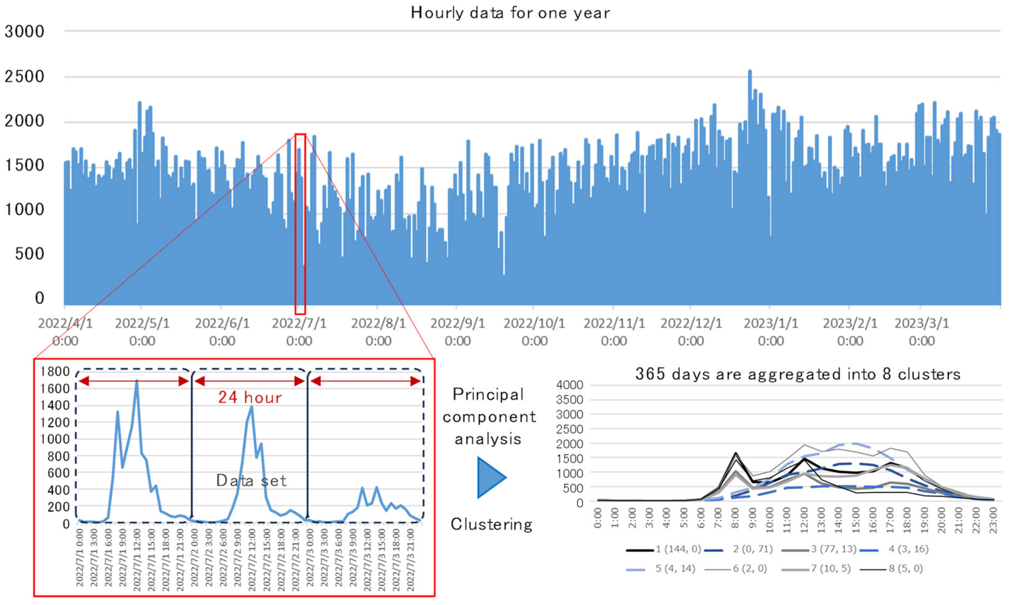
2.3. Analysis Method

A principal component analysis was performed on the hourly pedestrian counts from 0:00 to 23:00 on each day, considered as a 24-dimensional multivariate dataset [22]. The correlation matrix was used as the starting matrix. Principal components with eigenvalues greater than 1 were employed. As a result, the cumulative contribution was high, and most of the variation in the 24 variables was explained by a small number of principal components. Principal component scores were then computed and used in the hierarchical cluster analysis. Euclidean distance was used as the distance between samples, and the samples were classified using the mean linkage method between groups. From the dendrogram (tree diagram) obtained, the samples were classified into groups by drawing lines at certain distances so that the number of groups ranged from 3 to 10. Figure 2 shows the flow of principal component analysis and cluster classification.

2.4. Methods for Developing Thermal Environment Index Distribution

The distribution of the thermal environmental index in the same target area was developed for comparison with the results of the pedestrian count data analysis. The calculation method of the thermal environment index followed the method of previous studies by the authors, and the standard new effective temperature (SET*) was used as the thermal environment index [23,24,25]. Air temperature and humidity measurements at a height of 2 m and wind velocity 100 m above the ground at a meteorological observatory in early August were given, and solar radiation on a clear sky was set to calculate the distribution of solar radiation, ground surface temperature, and wind velocity, as affected by the shape of buildings and trees, and by surface cover conditions. The LES model was used to calculate the airflow distribution, and the time-averaged results of the unsteady calculations were used in the analysis. SET* was calculated assuming a metabolic rate of 1.4 met for walking and 0.6 clo for wearing clothes in the summer season.

3. Results

3.1. Principal Component Analysis and Cluster Classification Results

An example of the principal component analysis result at a certain measurement point is shown in Figure 3. The first principal component exhibited positive values throughout the day, with values exceeding 0.6 from 11:00 to 24:00. This component represents the overall magnitude of daily pedestrian counts. The second principal component showed values below −0.6 from 6:00 to 9:00 as well as negative values at 12:00 and from 17:00 to 20:00. This component captured the temporal variation in pedestrian activity, specifically the contrast between morning, afternoon, evening, and other periods. The variance explained by the first principal component was 53.5%, while the second accounted for 16.9%, resulting in a cumulative contribution exceeding 70%. At many measurement points, the principal component with positive values throughout the day and the principal component with negative values at morning, noon, and evening appeared. The daily magnitude and the morning, noon, and evening peaks of pedestrian numbers were considered to be dominant factors in the cluster classification. An example of the cluster classification result at a certain measurement point is shown in Figure 4. The peak time of day was the main factor in the cluster classification. Clusters with peaks during the commute to work or school were identified as weekday clusters, and clusters with peaks between 1:00 p.m. and 3:00 p.m. in the afternoon were identified as weekend clusters.

3.2. Typical Examples of Cluster Analysis Results

A typical example of the cluster classification results at the three measurement points is shown in Figure 5. The peak time of day was the main factor in the cluster classification. Clusters with peaks during commuting hours were identified as weekday clusters, while clusters with peaks between 1:00 p.m. and 3:00 p.m. were identified as weekend clusters. The legend below the graph indicates the cluster number (number of weekdays and number of weekends). Clusters with more weekdays are indicated by solid black lines, and clusters with more weekends are indicated by dashed blue lines. Clusters with no peaks are indicated by solid light-blue lines. Clusters with a mix of weekdays and weekends are indicated by red lines.

For the measurement point in Figure 5a, most days (335) were classified as Cluster 1 (solid light-blue line). At measurement points where many days were classified into one cluster, as in this example, the daily total number of pedestrians was small, and the difference between weekdays and weekends was not clear. Clusters 2 through 5 exhibited elevated pedestrian activity during daytime hours on weekends, likely influenced by social events. Cluster 6 showed increased pedestrian counts on weekday evenings, possibly reflecting special events, such as fireworks displays.

For the measurement point in Figure 5b, most days were classified as weekday Clusters 1, 3, 6, 7, and 8 (solid black lines) and weekend Clusters 2, 4, and 5 (dashed blue lines). At measurement points where many days were classified into two typical clusters (weekday and weekend), the daily total number of pedestrians was relatively large connected to the train stations. The clusters reflected peak activity during the morning, afternoon, and evening on weekdays, and during afternoon hours on weekends. The influence of long school vacations on weekday patterns and social events on holidays was also assumed.

For the measurement point in Figure 5c, Cluster 1 with a mix of weekdays and weekends (red lines) was identified, which had a large daily total number of pedestrians, with peaks for commuting to work and school as well as shopping and sightseeing. Cluster 2 showed elevated activity on weekday mornings and evenings. Clusters 3 through 6 displayed distinct peaks during the morning, afternoon, or evening on weekends, likely influenced by various social events.

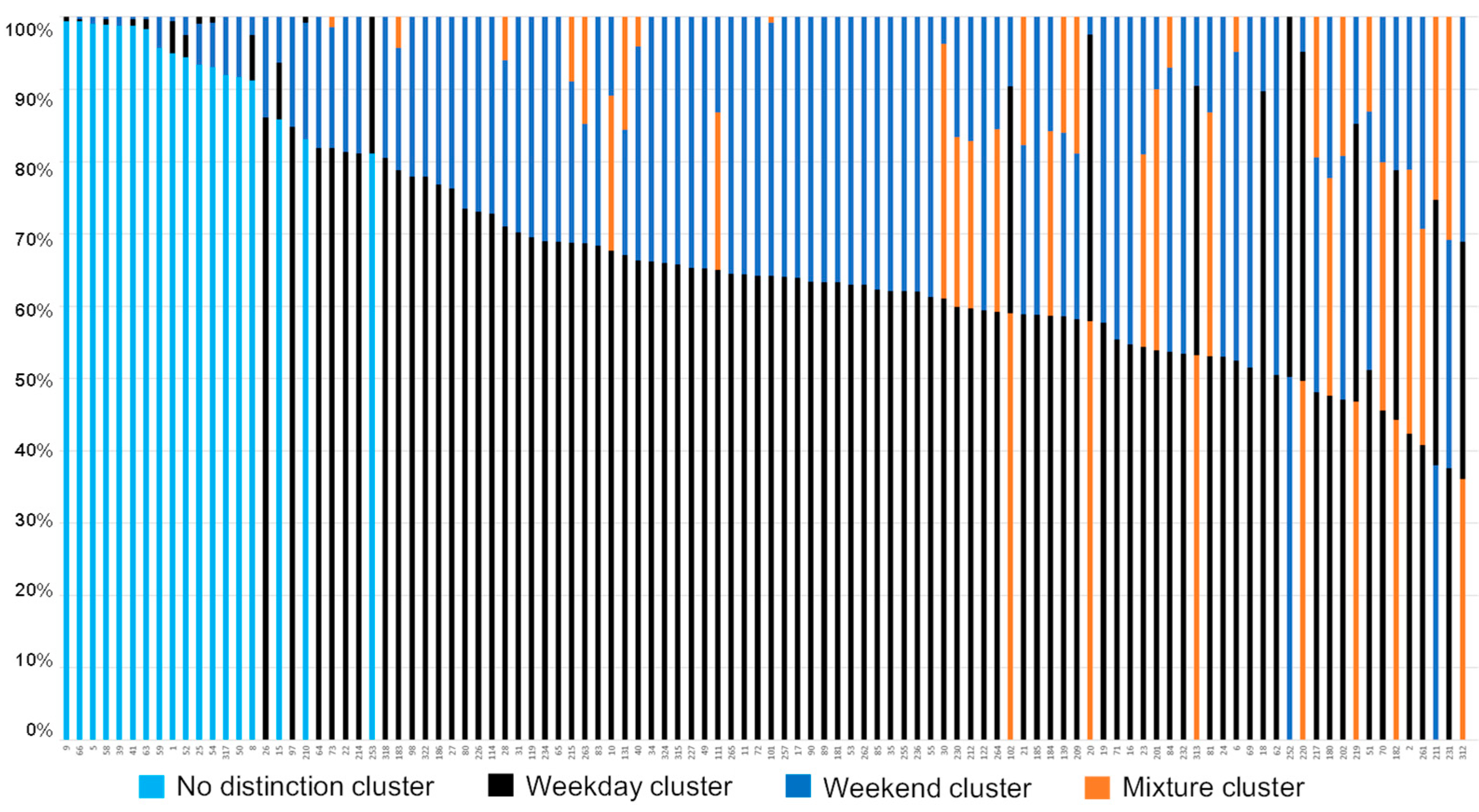
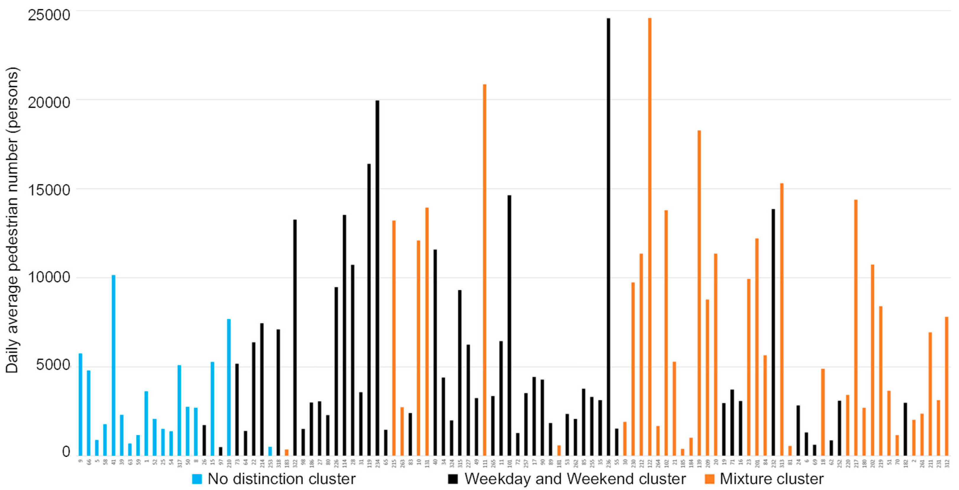
3.3. Percentage of Clusters

Figure 6 shows the percentage of clusters for all measurement points. The measurement points were sorted in the order of the largest percentage of clusters. No distinction clusters were dominant at 18 measurement points. Almost a single cluster occupied the most days at these points. About 50 measurement points were clearly divided into weekday and weekend clusters. Mixture clusters as well as weekday and weekend clusters were classified at about 40 measurement points.

Figure 7 shows the daily average pedestrian number, with the horizontal axis following Figure 6. Pedestrian number tended to be smaller at the measurement points with no distinction clusters and larger at the measurement points with mixture clusters.

Mapping of measurement points based on clustering results is shown in Figure 8. The circle size indicates the daily average pedestrian number. No distinction clusters (light blue) were plotted away from Sannomiya station and Motomachi station, and the daily average pedestrian number was small, at 3242 people. Most days (average 94%) were classified in one cluster. Weekday and weekend clusters were plotted close to the train stations to slightly further away and frequently corresponded to office districts. The daily average pedestrian numbers were 5410 on weekday clusters and 6167 on weekend clusters. The ratios of weekday and weekend clusters were 67% and 32%, respectively. Mixture clusters as well as weekday and weekend clusters were plotted close to the train stations and corresponded to office and commercial districts. The daily average pedestrian numbers were 6293 on weekday clusters, 9530 on weekend clusters, and 8887 on mixture clusters. The ratios of weekday, weekend, and mixture clusters were 51%, 21%, and 28%, respectively.

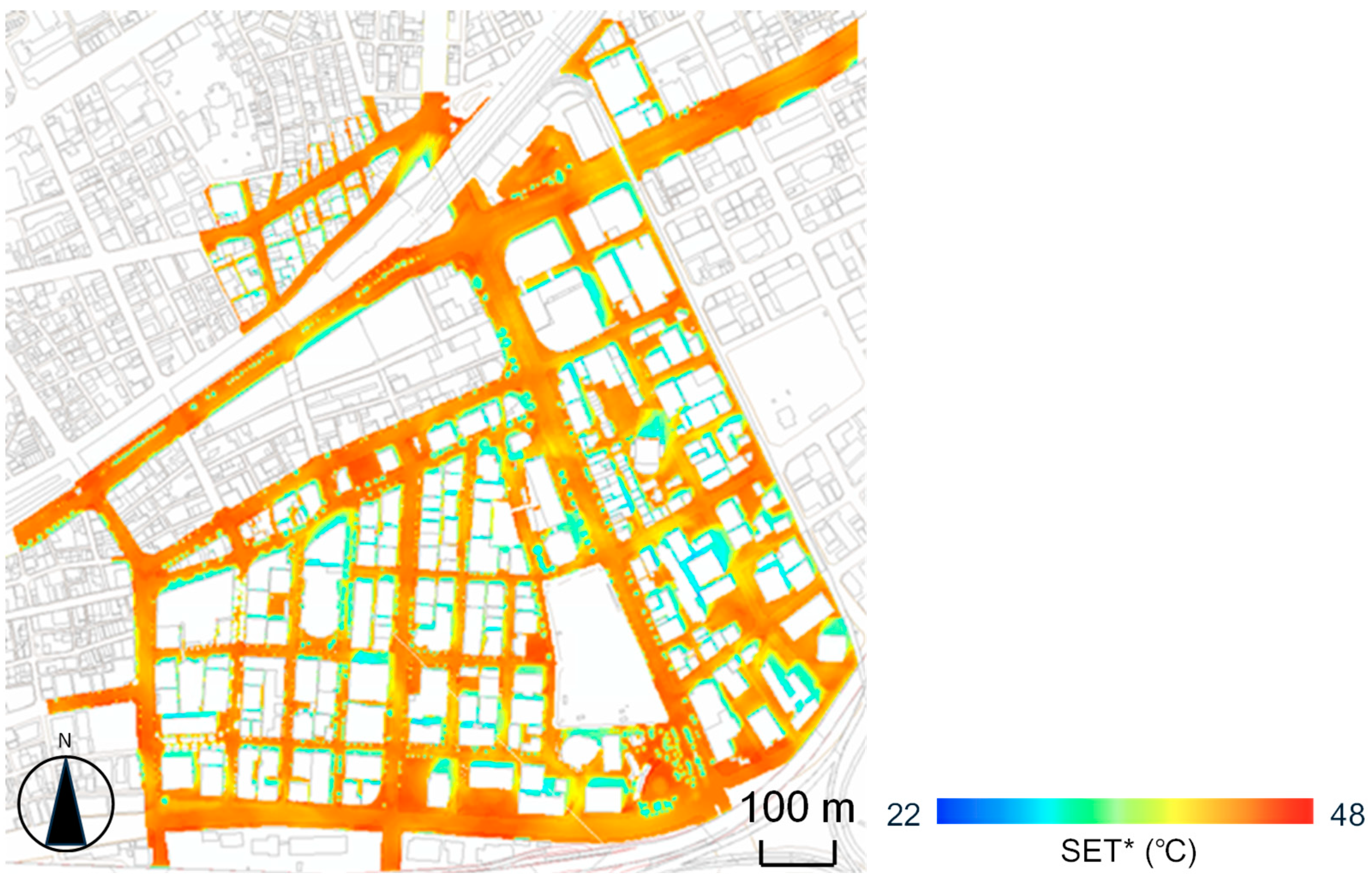
3.4. Calculation Results of SET* Distribution

The SET* distribution, calculated with a horizontal resolution of 2 m at a height of 1.5 m above ground with the settings of building geometry, surface coverage, and street tree distribution, is shown in Figure 9. Shading by buildings was the dominant influence on the distribution of thermal environmental indices. The hourly calculation results from 8:00 to 18:00 at measurement points of the pedestrian count data were analyzed using principal component analysis and cluster classification in the same way as for the pedestrian count data.

Classification results based on time variation of SET* at measurement points of the pedestrian count data are shown in Figure 10. The legend below the graph indicates the cluster number (number of measurement points). The characteristics of typical clusters are summarized below:

-

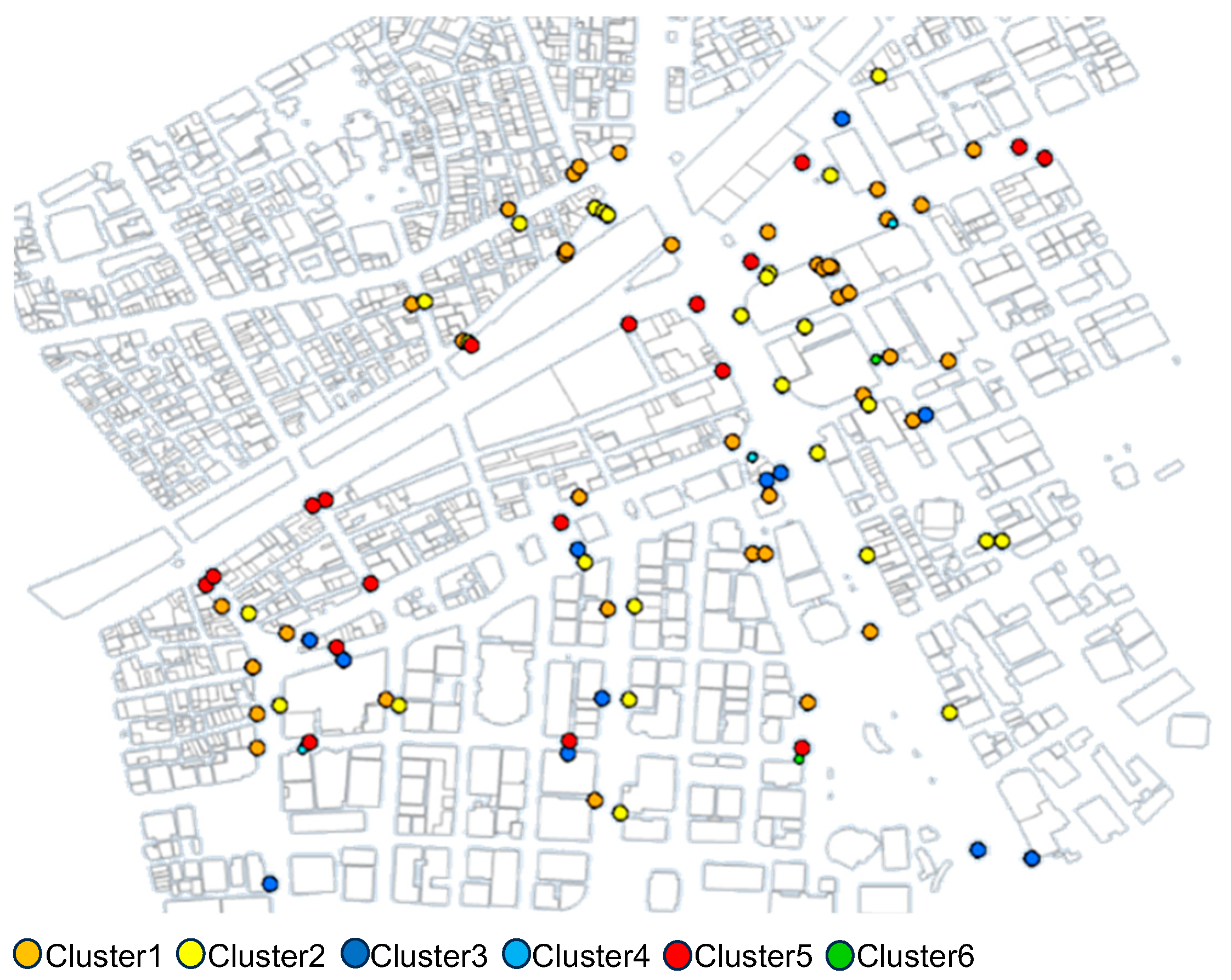
Cluster 1 had higher temperatures in the morning and was distributed on the west side of the north–south road.

-

Cluster 2 had higher temperatures in the afternoon and was distributed on the east side of the north–south road.

-

Cluster 3 had lower temperatures throughout the day and was distributed on the south side of the east–west road.

-

Cluster 5 had higher temperatures throughout the day and was distributed on the north side of the east–west road and on the wider road.

Clusters 4 and 6 have fewer classifications.

Mapping of measurement points based on SET* clustering results is shown in Figure 11. The spatial distribution was generally classified by the east and west sides of the north–south road, and the north and south sides of the east–west road, but there was some variation depending on the surrounding buildings.

4. Discussion

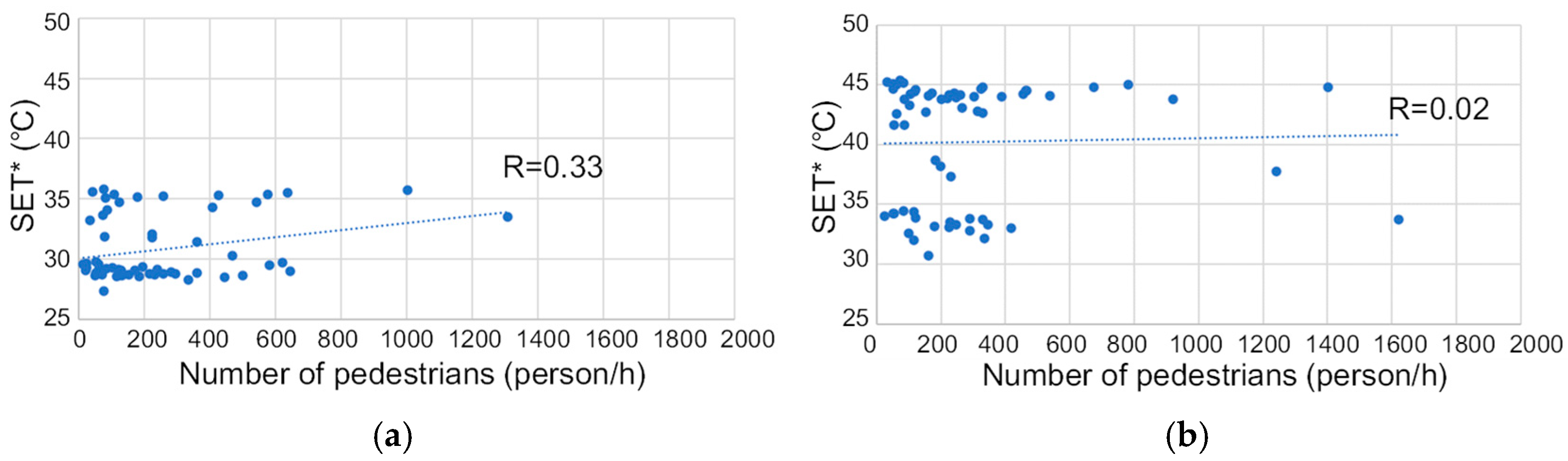
4.1. Relationship Between Pedestrian Count Data Analysis and Thermal Environment Analysis

The results of the principal component analysis and cluster analysis did not confirm a significant influence of the thermal environment on the temporal variation characteristics of pedestrian count data. This suggested that the distinction between weekdays and holidays played a dominant role in shaping the 24 h and year-round patterns, whereas the effects of season and weather were relatively minor. Indeed, as shown in Figure 12, no correlation was observed between the number of pedestrians and SET* at either 8:00 or 13:00. SET* was higher in the sunny areas and lower in the shaded areas, but pedestrians behaved independently of these conditions. However, in more confined spaces—such as station plazas, pedestrian pathways, or inner-city parks—the relationship between pedestrian counts and thermal environment indices, based on CFD and mutual radiation exchange, could be explored at a finer spatial resolution. Watanabe and Ishii [26] analyzed the effects of microclimatic conditions on shade-selective behavior of pedestrians waiting at traffic lights in the subtropical city of Nagoya and noted that urban shade design would be an important strategy for improving urban safety, comfort, and attractiveness in a hot climate.

4.2. Temporal Characteristics of Pedestrian Count Data and Thermal Environmental Indices

By comparing temporal variation characteristics (Figure 5b and Figure 10), temporal strategies for measuring high temperatures can be considered. By comparing spatial distribution characteristics (Figure 8 and Figure 11), spatial strategies for measuring high temperatures can be considered. These figures are reproduced in Figure 13.

The temporal characteristics of the pedestrian count data were classified into weekday and weekend clusters according to the peak hours within a day. Hirose et al. [18] and Imai et al. [19] analyzed the behavioral characteristics according to the objectives of tourists and public transport, respectively, and it was clear that their objectives were superior to weather conditions and other factors. Kumakura et al. [20] analyzed the data considering the effects of age group, activity status, and weather conditions, suggesting the possibility of a detailed analysis if data were obtained at a more detailed spatial resolution. The temporal characteristics of thermal environmental index SET* were classified according to sidewalk location. These relationships were clearly independent, and the time of high risk for many pedestrians exposed to high temperatures was identified based on the results of the analysis for each location. However, it was possible to identify approximate tendencies in the following groups: weekdays and holidays, north and south sides of east–west roads, and east and west sides of north–south roads.

4.3. Spatial Characteristics of Pedestrian Count Data and Thermal Environmental Indices

The spatial characteristics of the pedestrian count data were clearly defined by distance from the station, office district, and commercial district, according to peak commuting, shopping, etc. Zhang and Ludwig [27] used hourly boarding and exiting data from subway stations, but their analysis did not use actual city data because the behavioral conditions within the urban area were assigned considering the typical commuting patterns of students and workers on weekdays. The spatial characteristics of thermal environmental index SET* were classified according to shadows by surrounding buildings. These relationships were clearly independent, and the time of high risk for many pedestrians exposed to high temperatures was identified based on the results of the analysis for each location. However, it was possible to identify approximate tendencies in the following groups: near the station, in offices or the commercial district, north and south sides of east–west roads, and east and west sides of north–south roads.

4.4. Limitations and Relevance of This Study

In this study, pedestrian count data obtained via infrared sensors using existing sensing technology and the calculated spatiotemporal distribution of the thermal environment index SET*—for which extensive research has been accumulated—were analyzed using established statistical methods, such as principal component analysis and cluster classification. Some intuitively expected patterns were identified; for example, pedestrian behavior influenced by commuting was observed on weekdays. Although the methods and findings are not novel, the approach represents a valuable practical contribution that can be applied to other urban contexts as well.

The temporal characteristics of the thermal environmental indices were classified into four clusters:

(1)

high temperatures in the morning on the west sidewalk of the north–south road,

(2)

high temperatures in the afternoon on the east sidewalk of the north–south road,

(3)

low temperatures throughout the day on the south sidewalk of the east–west road,

(4)

high temperatures throughout the day on the north sidewalk of the east–west road and on sidewalks along wide roads.

These classification results were characterized by a clear correspondence between temporal and spatial distribution patterns. Although such patterns have been noted in previous studies [8,9,10,11,12,13,14,15,16,17], they were statistically extracted in this study from spatial distribution data collected at various points in an actual urban area. Therefore, the findings can be regarded as persuasive evidence for urban environmental planning.

The results of a one-year statistical analysis of hourly pedestrian counts, obtained from sensors installed at more than 100 locations, provide valuable insights into pedestrian behavior in urban areas. However, collecting data related to thermal environmental indices at a similar spatial and temporal resolution remains challenging. This difficulty arises because it is not feasible to remotely measure variables such as air temperature, humidity, wind velocity, and mean radiant temperature—unlike pedestrian counts, which can be measured remotely using infrastructure like streetlights. While infrared thermal cameras can be deployed at multiple locations to measure surface temperature distributions, which are closely related to mean radiant temperature, pedestrian count data serve multiple purposes, including urban safety and commercial activity. As a result, there is limited incentive to develop dedicated infrastructure solely for thermal environmental assessment.

5. Conclusions

A temporal and spatial analysis method was examined for the purpose of thermal environment planning using hourly pedestrian count data over the year provided by Kobe City at more than 100 locations in the street canyon. A principal component analysis was performed on the hourly number of pedestrians between 0:00 and 23:00 on each day, considering it as a 24-dimensional multivariate dataset. At many measurement points, the principal component with positive values throughout the day and the principal component with negative values at morning, noon, and evening appeared. Clusters with peaks during the commute to work or school were identified as weekday clusters, and clusters with peaks between 1:00 p.m. and 3:00 p.m. in the afternoon were identified as weekend clusters.

More than 100 measurement points were classified into 3 major groups. At measurement points where many days were classified into one cluster, the daily total number of pedestrians was small, and the difference between weekdays and weekends was not clear. At measurement points where many days were classified into two typical clusters (weekday and weekend), the daily total number of pedestrians was relatively large connected to the train stations. Measurement points where clusters with a mixture of weekdays and weekends were identified had a large daily total number of pedestrians, with peaks for commuting to work and school, as well as shopping and sightseeing.

Measurement points were also classified based on time variation of SET*. The spatial distribution was generally classified by the east and west sides of the north–south road, and the north and south sides of the east–west road, but there was some variation depending on the surrounding buildings.

The temporal characteristics of the pedestrian count data were classified into weekday and weekend clusters according to the peak hours within a day. The spatial characteristics of the pedestrian count data were clearly defined by distance from the station, office district, and commercial district, according to peak commuting, shopping, etc. Spatiotemporal characteristics of the thermal index SET* were analyzed in the same way and were classified mainly according to the characteristics of solar radiation shielding by surrounding buildings.

Results from principal component analysis and cluster analysis did not reveal a significant influence of the thermal environment on the temporal variation in pedestrian counts. Instead, the data suggested that weekday versus weekend distinctions were the primary determinants of daily and annual patterns, while seasonal and weather-related factors had relatively minor effects. The analytical approach developed in this study represents a valuable and practical contribution that may be applicable to other urban contexts as well.

References

1. Kearl, Z.; Vogel, J. Urban extreme heat, climate change, and saving lives: Lessons from Washington state. Urban Clim. 2023, 47, 101392. [Google Scholar] [CrossRef]
2. Heat Illness Prevention Information. Available online: https://www.wbgt.env.go.jp/en/ (accessed on 26 March 2025).
3. Kenny, G.P.; Yardley, J.; Brown, C.; Sigal, R.J.; Jay, O. Heat stress in older individuals and patients with common chronic diseases. Can. Med. Assoc. J. 2010, 182, 1053–1060. [Google Scholar] [CrossRef] [PubMed]
4. Vandentorren, S.; Bretin, P.; Zeghnoun, A.; Mandereau-Bruno, L.; Croisier, A.; Cochet, C.; Ribéron, J.; Siberan, L.; Declercq, B.; Ledrans, M. August 2003 heat wave in France: Risk factors for death of elderly people living at home. Eur. J. Public Health 2006, 16, 583–591. [Google Scholar] [CrossRef] [PubMed]
5. Nayak, S.G.; Shrestha, S.; Sheridan, S.C.; Hsu, W.H.; Muscatiello, N.A.; Pantea, C.I.; Ross, Z.; Kinney, P.L.; Zdeb, M.; Hwang, S.A.; et al. Accessibility of cooling centers to heat-vulnerable populations in New York state. J. Transp. Health 2019, 14, 100563. [Google Scholar] [CrossRef] [PubMed]
6. Lee, K.; Chae, Y. Analysis of socioeconomic disparities and accessibility to cooling centers using travel time of 100 m × 100 m grids in South Korea. Urban Clim. 2021, 36, 100762. [Google Scholar] [CrossRef]
7. Heat Countermeasure Guideline in the City. Available online: https://www.wbgt.env.go.jp/pdf/city_gline/city_guideline_full.pdf (accessed on 26 March 2025).
8. Nikolopoulou, M.; Lykoudis, S. Thermal comfort in outdoor urban spaces: Analysis across different European countries. Build. Environ. 2006, 41, 1455–1470. [Google Scholar] [CrossRef]
9. Johansson, E. Influence of urban geometry on outdoor thermal comfort in a hot dry climate: A study in Fez, Morocco. Build. Environ. 2006, 41, 1326–1338. [Google Scholar] [CrossRef]
10. Johansson, E.; Emmanuel, R. The influence of urban design on outdoor thermal comfort in the hot, humid city of Colombo, Sri Lanka. Int. J. Biometeorol. 2006, 51, 119–133. [Google Scholar] [CrossRef] [PubMed]
11. Ali-Toudert, F.; Mayer, H. Numerical study on the effects of aspect ratio and orientation of an urban street canyon on outdoor thermal comfort in hot and dry climate. Build. Environ. 2006, 41, 94–108. [Google Scholar] [CrossRef]
12. Ali-Toudert, F.; Mayer, H. Effects of asymmetry, galleries, overhanging facades and vegetation on thermal comfort in urban street canyons. Sol. Energy 2007, 81, 742–754. [Google Scholar] [CrossRef]
13. Ali-Toudert, F.; Mayer, H. Thermal comfort in an east–west oriented street canyon in Freiburg (Germany) under hot summer conditions. Theor. Appl. Climatol. 2007, 87, 223–237. [Google Scholar] [CrossRef]
14. Emmanuel, R.; Rosenlund, H.; Johansson, E. Urban shading—A design option for the tropics? A study in Colombo, Sri Lanka. Int. J. Climatol. 2007, 27, 1995–2004. [Google Scholar] [CrossRef]
15. Hwang, R.L.; Lin, T.P.; Matzarakis, A. Seasonal effects of urban street shading on long-term outdoor thermal comfort. Build. Environ. 2011, 46, 863–870. [Google Scholar] [CrossRef]
16. Takebayashi, H.; Moriyama, M. Relationships between the properties of an urban street canyon and its radiant environment: Introduction of appropriate urban heat island mitigation technologies. Sol. Energy 2012, 86, 2255–2262. [Google Scholar] [CrossRef]
17. Lindberg, F.; Thorsson, S.; Rayner, D.; Lau, K. The impact of urban planning strategies on heat stress in a climate-change perspective. Sustain. Cities Soc. 2016, 25, 1–12. [Google Scholar] [CrossRef]
18. Hirose, T.; Imura, S.; Kinuta, Y.; Yabe, T. Understanding Tourists’ Activity through Analyzing Smartphone Data. In IBS Annual Report; The Institute of Behavioral Science: Tokyo, Japan, 2019; pp. 43–50. [Google Scholar]
19. Imai, R.; Fukada, M.; Shigetaka, K.; Yabe, T.; Makimura, K.; Adachi, R. Feasibility study on applicability of multi-tail data using combinational analysis in urban transportation planning. In Proceedings of the 47th Annual Conference on Civil Engineering and Planning, Hiroshima, Japan, 1–2 June 2013; pp. 1–9. [Google Scholar]
20. Kumakura, E.; Ashie, Y.; Ueno, T. Research on the Heat Risk Related to Urban Heat Islands, Part 2: Analysis of Population Flow Data, Summaries of Technical Papers of Annual Meeting Architectural Institute of Japan; Architectural Institute of Japan: Tokyo, Japan, 2022; Volume D-1, pp. 2125–2126. [Google Scholar]
21. Sensors & Work. Available online: https://www.sensorsandworks.com (accessed on 26 March 2025).
22. Yanai, H. Handbook of Multivariate Analysis; Gendai-Sugakusha: Kyoto, Japan, 1986; pp. 70–80+224–242. [Google Scholar]
23. Takebayashi, H. Thermal environment design of outdoor spaces by examining redevelopment buildings opposite central Osaka station. Climate 2019, 7, 143. [Google Scholar] [CrossRef]
24. Takebayashi, H.; Okubo, M.; Danno, H. Thermal environment map in street canyon for implementing extreme high temperature measures. Atmosphere 2020, 11, 550. [Google Scholar] [CrossRef]
25. Takebayashi, H.; Danno, H.; Tozawa, U. Study on strategies to implement adaptation measures for extreme high temperatures into the street canyon. Atmosphere 2022, 13, 946. [Google Scholar] [CrossRef]
26. Watanabe, S.; Ishii, J. Effect of outdoor thermal environment on pedestrians’ behavior selecting a shaded area in a humid subtropical region. Build. Environ. 2016, 95, 32–41. [Google Scholar] [CrossRef]
27. Zhang, X.; Ludwig, F. Shade for pedestrians: A novel approach to calculate the spatio-temporal shade benefits of street trees considering pedestrian flow. Build. Environ. 2025, 272, 112662. [Google Scholar] [CrossRef]
Figure 1. Location (red dots), photograph, and installation status of infrared sensors (approximately 1 km2).
Atmosphere 16 00504 g001
Figure 2. Flow of principal component analysis and cluster classification.
Atmosphere 16 00504 g002
Figure 3. Example of the principal component analysis result at a certain measurement point.
Atmosphere 16 00504 g003
Figure 4. Example of the cluster classification result at a certain measurement point (red dot in right map). The legend below the graph indicates the cluster number (number of weekdays and number of weekends). Clusters with more weekdays are indicated by solid black lines, and clusters with more weekends are indicated by dashed blue lines.
Atmosphere 16 00504 g004
Figure 5. Typical examples of the cluster classification results at three measurement points (red dot in right map): (a) at a measurement point where most days were classified as weekday clusters, (b) at a measurement point where most days were classified as weekday clusters, and (c) at a measurement point where clusters with a mix of weekdays and weekends were identified.
Atmosphere 16 00504 g005
Figure 6. Percentage of clusters for all measurement points. The measurement points are sorted in the order of the largest percentage of clusters.
Atmosphere 16 00504 g006
Figure 7. Daily average pedestrian number for all measurement points. The horizontal axis follows Figure 6.
Atmosphere 16 00504 g007
Figure 8. Mapping of measurement points based on clustering results of pedestrian numbers (approximately 1 km2). The circle size indicates the daily average pedestrian number.
Atmosphere 16 00504 g008
Figure 9. Calculation results of SET* distribution at 13:00 in early August at the pedestrian level (1.5 m high) in the targeted area (approximately 1 km2).
Atmosphere 16 00504 g009
Figure 10. Classification results based on time variation of SET* at measurement points of the pedestrian count data. The legend below the graph indicates the cluster numbers (number of measurement points).
Atmosphere 16 00504 g010
Figure 11. Mapping of measurement points based on SET* clustering results (approximately 1 km2).
Atmosphere 16 00504 g011
Figure 12. Correlation between the number of pedestrians and SET* at (a) 8:00 and (b) 13:00.
Atmosphere 16 00504 g012
Figure 13. Comparison of temporal variation and spatial distribution of pedestrian count data and thermal environmental indices (approximately 1 km square). (a) Comparison of temporal variation characteristics (Figure 5b and Figure 10 reproduced). (b) Comparison of spatial distribution characteristics (Figure 8 and Figure 11 reproduced). The circle size indicates the daily average pedestrian number.
Atmosphere 16 00504 g013