Abstract
The transferability of the regional climate model REMO with a standard setup over different regions of the world has been evaluated. The study is based on the idea that the modeling parameters and parameterizations in a regional climate model should be robust to adequately simulate the major climatic characteristic of different regions around the globe. If a model is not able to do that, there might be a chance of an “overtuning” to the “home-region”, which means that the model physics are tuned in a way that it might cover some more fundamental errors, e.g., in the dynamics. All simulations carried out in this study contribute to the joint effort by the international regional downscaling community called COordinated Regional climate Downscaling EXperiment (CORDEX). REMO has been integrated over six CORDEX domains forced with the so-called perfect boundary conditions obtained from the global reanalysis dataset ERA-Interim for the period 1989 to 2008. These six domains include Africa, Europe, North America, South America, West Asia and the Mediterranean region. Each of the six simulations was conducted with the identical model setup which allows investigating the transferability of a single model to regions with substantially different climate characteristics. For the consistent evaluation over the different domains, a new evaluation framework is presented by combining the Köppen-Trewartha climate classification with temperature-precipitation relationship plots and a probability density function (PDF) skill score method. The evaluation of the spatial and temporal characteristics of simulated precipitation and temperature, in comparison to observational datasets, shows that REMO is able to simulate the mean annual climatic features over all the domains quite reasonably, but still some biases remain. The regions over the Amazon and near the coast of major upwelling regions have a significant warm bias. Wet and dry biases appear over the mountainous regions and East Africa, respectively. The temperature over South America and precipitation over the tundra and highland climate of West Asia are misrepresented. The probable causes leading to these biases are discussed and ideas for improvements are suggested. The annual cycle of precipitation and temperature of major catchments in each domain are also well represented by REMO. The model has performed well in simulating the inter- and intra-seasonal characteristics of different climate types in different regions. Moreover, the model has a high ability in representing the general characteristics of different climate types as measured by the probability density function (PDF) skill score method. Although REMO seems to perform best over its home domain in Europe (domain of development and testing), the model has simulated quite well the climate characteristics of other regions with the same set of parameterization options. Therefore, these results lead us to the conclusion that REMO is well suited for long-term climate change simulations to examine projected future changes in all these regions.
1. Introduction
In order to provide an ensemble of high-resolution, regional climate projections for all major continental regions of the world, the World Climate Research Program (WCRP) has initiated a coordinated effort by the International Regional Downscaling Community to downscale the CMIP5 (Coupled Model Intercomparison Project Phase 5) scenarios. This effort, referred to as CORDEX (COordinated Regional climate Downscaling EXperiment), currently involves more than 20 Regional Climate Model (RCM) groups around the world. The goal is to provide a quality-controlled data set of downscaled information for the recent historical past and 21st century projections, covering the majority of populated land regions around the globe. The coordination of different regional climate simulations for 12 defined domains [1] reinforced by reanalysis data shall provide a benchmark framework for model evaluation and assessment.
In the framework of CORDEX, the regional climate model REMO [2] is applied over Africa (mandatory domain), Europe, North America, South America, West Asia and the Mediterranean region. The aim is to produce an ensemble of regional climate change simulations with REMO over multiple domains driven by different General Circulation Models (GCMs) from the CMIP5 archive, in order to provide the high resolution climate change information for further impact and adaptation studies. However, as a first step, the evaluation of the ability of REMO to capture the climate features of the above-mentioned regions has to be done. Therefore, REMO has been integrated using reanalysis data [3] as boundary forcing to evaluate its performance against observations in present climate.
In an earlier study carried out by Takle et al. [4] the transferability of five RCMs to different domains around the world, keeping identical modeling parameters and parameterization, was tested. It was found that the RCMs perform better in the domain for which they were originally developed and show reduced accuracy in non-native domains. However, in transient climate projections, the major climate characteristics of a region might undergo a significant change. Hence a model setup that is fitted to best reproduce the current climate characteristics of a region might fail in doing so in the future. In retrospect, a model setup that reasonably reproduces well the current climate in the mid-latitudes and also in the subtropical and tropical areas might be superior to any domain specific setup. Therefore, in order to evaluate the transferability of REMO to different domains, the model parameterization such as the convection scheme and boundary layer scheme are not adapted to the specific domains but used the same standard setup for all simulations. Originally, REMO has been developed and tested for Europe [5].
To estimate if the chosen model setup is transferable to all of the six investigated CORDEX domains, the simulated climate characteristics in each model domain are evaluated against observed data. The mean temperature and precipitation characteristics are analyzed and presented in a global overview. Moreover, the performance of REMO in capturing the annual cycles of precipitation and temperature of selected catchments in each domain is also evaluated against observations. For a consistent evaluation of an RCM across different domains, an evaluation framework needs to be defined. Such a framework will not only give insights into the model performance over the different regions, but will also allow a quantitative comparison between them. From this comparison, conclusions on transferability of the RCM to different domains can be drawn. In the evaluation introduced in the present study, we focus on temperature and precipitation characteristics in different climate types defined by the Köppen-Trewartha climate classification [6]. This allows a good assessment for the regional climate model performance in different regions and in different climate types. The skill of the model is analyzed by precipitation-temperature relationship plots and further quantified by the evaluation of probability density functions (PDF) for each climate type and each region following the PDF skill score method discussed in Perkins et al. [7].
A brief description of REMO and the experiment design is given in Section 2. This is followed by the evaluation framework for validation of model over different regions (Section 3). The discussions of results are in Section 4 and the final considerations in the current research are presented in Section 5.
2. Model and Experiment Setup
In this study, the regional climate model REMO is used in its most recent hydrostatic version (REMO 2009) [5,8]. It was originally developed over Europe using the physical parameterizations of ECHAM 4 [9] and the dynamical core of the former weather prediction model of the German Weather Service (DWD) [10]. An overview of the model specifications is given in Table 1.

Table 1.
Summary of the REMO specifications used for the COordinated Regional Climate Downscaling EXperiment (CORDEX) simulations.
| Model Version | Vertical Coordinate/Levels | Advection Scheme | Time Step | Convective Scheme | Radiation Scheme | Turbulence Vertical Diffusion | Cloud Microphysics Scheme | Land Surface Scheme |
|---|---|---|---|---|---|---|---|---|
| REMO 2009 hydrostatic | Hybrid/ 27-31 | Semi-lagrangian | 240 s | Tiedtke [11], Nordeng [12], Pfeifer [13] | Morcrette et al. [14], Giorgetta and Wild [15] | Louis [16] | Lohmann and Roeckner [17] | Hagemann [18], Rechid et al. [19] |
As mentioned earlier, the large-scale forcing of the regional climate model is taken from the global reanalysis data of ERA-Interim [3] at a horizontal resolution of approx. 0.7° × 0.7° and interpolated to all the six model domains in which REMO simulations are performed for the entire time period from 1989 to 2008. The forcing data is prescribed at the lateral boundaries of each domain with an exponential decrease towards the center of the model domain. The main direct influence of the boundary data lies in the eight outer grid boxes using a relaxation scheme according to Davies [20]. A subset of 6 out of 12 CORDEX domains shown in Figure 1 is downscaled in the present study namely Africa, Europe, the Mediterranean region, North America, South America and West Asia. The downscaling is conducted to a horizontal resolution of 0.44° × 0.44° (approx. 50 × 50 km2) using the same model parameterizations in each domain.
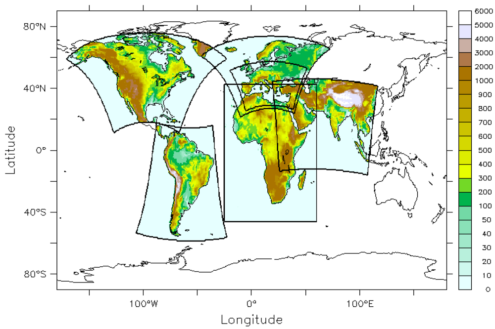
Figure 1.
Orography (m) of the 6 COordinated Regional Climate Downscaling EXperiment (CORDEX) model domains.
Figure 1.
Orography (m) of the 6 COordinated Regional Climate Downscaling EXperiment (CORDEX) model domains.

3. Evaluation Framework
To assess the quality of the REMO simulations over the different domains, the monthly mean temperature and the monthly total precipitation from the CRUv3.0 (referred to CRU hereafter) observational dataset [21] are used. The data is aggregated onto a 0.5° × 0.5° global grid over land areas only and has been analyzed extensively by Brohan et al. [22]. In order to take into account differences in the orography between REMO and CRU, temperature values are height-corrected. It must be noted here that the CRU precipitation data are uncorrected for the precipitation undercatch of measurement gauges, which is especially important in mountainous areas and for snowfall where underestimations of up to 40% may occur [23].
To group the data of the different domains, the climate type classification after Köppen-Trewartha [6] is utilized. A similar classification approach is applied by Lohmann et al. [24] for the validation of a GCM. This approach is used to identify regions with similar mean climate conditions and also similar predominant climatic features, e.g., convective rain formation in the tropical regions versus advective processes in the temperate zones. For this study, the classification is based on a 30-year monthly time series of global CRU temperature and precipitation data for the period 1901 to 2006. The definition of Köppen-Trewartha climate types and their global distribution according to CRU data are illustrated in Figure 2. Details on the allocation of the climate types can be found in Trewartha [6], or in de Castro et al. [25]. For each of the climate types, a mask is generated and is subsequently applied to all the CORDEX domains simulated with REMO in order to group the model data of the different domains for analysis. For domains with a large overlapping area such as in the case of the African and the West Asian domain, only grid points belonging to the respective continent are taken into account. Moreover, all regions attributed to a climate type (according to CRU) that is below an areal fraction of 5% of all land points of the respective domain are excluded from the analysis. This threshold is introduced to only consider climate types that are representative for the respective domain. Based on this data, the correlation of monthly mean precipitation and temperature data are compared between the simulation results and the CRU observations for all climate types and domains from 1989 to 2006.
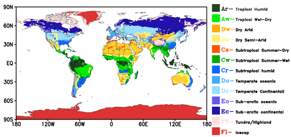
Figure 2.
The derived Köppen-Trewartha (K-T) climate classification based on the 30-year mean of the CRUv3.0 dataset.
Figure 2.
The derived Köppen-Trewartha (K-T) climate classification based on the 30-year mean of the CRUv3.0 dataset.

To receive a quantitative measure of the model quality, the skill of the model is additionally evaluated to represent the mean climate characteristics for each climate type and domain. The score is quantified using the empirical probability density functions (PDF) of observed and simulated time series of monthly precipitation and temperature data. The PDF skill score (Sscore) follows the methods employed in Perkins et al. [7] and Tapiador et al. [26]. It measures the cumulative minimum probability between the normalized PDFs of observation and model data. Sscore represents the common area between the two PDF distributions and is defined as:
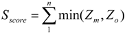
where n is the number of bins used to calculate the PDF for a given region, and Zm and Zo are the frequency of model values and observed values in a given bin, respectively [7]. This simple method gives a robust comparison of the similarity between the PDF of the model values and the observed values. A perfect score of one indicates that the distribution of the model is exactly the same as the observed distribution. A score less than one indicates that the model is not able to reproduce the distribution of the observations to the full extent.
The PDFs are calculated using 0.1 °C and 1 mm/day bin sizes for temperature and precipitation, respectively. The novel idea in using the PDF skill score method is its selection of regions according to the climate classification after Köppen-Trewartha. This setup allows to quantitatively compare the performance of REMO over different climate zones in each domain. In addition to the Sscore for each climate zone, a weighted mean skill score is calculated across the different domains. The weights are proportional to the number of grid points for each climate type in a particular domain. This means that for each climate zone, the region with a large number of grid points contributes more to the mean skill score. Hence, the calculated skill of the model in representing different climates throughout the globe will substantiate the transferability of REMO.
4. Evaluation of Model Results
4.1. Global Temperature and Precipitation Characteristics
The differences between simulated and observed (CRU) annual mean air temperature (2 m height) over all six domains are shown in Figure 3(a). Regions where the model is doing relatively well can be found in Europe, western Africa, eastern North America and south eastern South America. In these regions, the temperatures do not deviate more than one degree from observations. Taking into consideration that the annual mean temperature may not reveal all regional or temporal shortcomings, there are only a few regions where the model shows problematic behavior. First, the Amazonian forest area in South America has a considerable warm bias around 2 to 3 °C over a large area. The reasons are not yet fully understood but it may be attributed to insufficient local moisture recycling, especially in the dry season in the boreal summer. Here, it seems that the one-layer soil water storage of REMO does not take into account the buffering effect of water in deeper layers of the soil that may be accessed for transpiration by the vegetation in dry season, as investigated in the study of Kleidon and Heimann [27]. Second, the strong cold bias in the Himalayan region may be a model artifact to some degree, but also the observation data sparseness in that region seems to play a major role in emphasizing this feature. Third, the distinct warm bias north of the Hudson Bay in North America may have two reasons. One reason is the insufficient temperature representation of the Hudson Bay water body and the other may be concerned with an insufficient snow masking in that region.
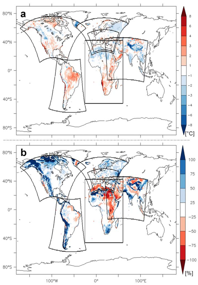
Figure 3.
(a) Differences of simulated and observed (CRU) annual mean air temperature (2 m height) in [°C]; (b) Relative annual mean differences between simulated and observed (CRU) precipitation in [%]. The period considered is 1989 to 2006.
Figure 3.
(a) Differences of simulated and observed (CRU) annual mean air temperature (2 m height) in [°C]; (b) Relative annual mean differences between simulated and observed (CRU) precipitation in [%]. The period considered is 1989 to 2006.

In Figure 3(a), strong surface warm biases are detected in coastal areas of Baja California (North America), Santiago de Chile up to Ecuador (South America) and the Namib Desert (Africa). In particular, the temperatures alongshore the Benguela Ocean current are far too warm all year round. The common characteristics of these regions are the upwelling of cold water and the subsidence of warm and dry air, driven by the Hadley circulation. This creates a thin inversion layer where stratocumulus clouds are formed. The simulated warm bias could be related to the misrepresentation of stratocumulus clouds and therefore an overestimation of radiation input to the surface as it already has been discussed in Haensler et al. [28] for the southern African region and/or wrong sea surface temperatures from the driving ERA-Interim data set [29,30].
In Figure 3(b), relative annual mean precipitation differences between simulated and observed (CRU) precipitation are shown. A prominent systematic feature is the occurrence of biases above hundred percent in dry regions. These can be related to the standardization method that is applied to the data and to the division by small values resulting in huge percentage differences. Apart from that, a prominent bias is the strong overestimation of rainfall up to 100% in the western mountain chains in the Americas and in the North American Arctic regions. To some degree, the latter error may be connected to the undercatch of the observing stations, which can lead to underestimation of precipitation in the annual observations by up to 40% [23]. Yang et al. [31] show that the correction factors for precipitation can reach monthly values of more than 100% during the winter season at high latitudes. This is the period in which REMO precipitation bias in comparison to CRU is highest (not shown). Regions, where precipitation is underestimated by up to 75%, are located in eastern and northern Africa and on the Arabic Peninsula. The distinct dipole error pattern over India with underestimation of precipitation in the northeast and overestimation over central India can be attributed to insufficiently characterized monsoon features and flow directions. In other regions, the model simulates the precipitation in Europe, eastern North America, eastern South America, western and south-western Africa quite well.
A general systematic inverse correlation of temperature bias to precipitation bias is not directly detected. In some regions such as India and eastern Central Europe, this assumption is true where a wet bias corresponds to a cold bias. In most regions, the picture looks quite non-systematic. For example, a warm bias corresponds to a wet bias in southern Africa and arctic North America. Inversely, a cold bias is associated with a dry bias in North Africa.
As mentioned earlier that to a large extent, the evaluation of the model is hampered by the lack of observational data. An example in this regard is the West Asian’s wet bias in REMO for the climate type Dc for the month December–February as given in Table 2. This region receives considerable amount of precipitation from western disturbances in these months, and it can be seen in Figure 2 that most of this climate type is present in Afghanistan or at very high altitudes over Pakistan. The lack of appropriate observational data in these regions is responsible for this particular bias.
One of the main objectives of the CORDEX experiment is to produce high-resolution regional climate change information as input to climate impact research and adaptation work. Many impact models need such information on river basin scale. Therefore in this study, the annual cycles of precipitation and temperature (2 m height) over the representative river basins for each domain are analysed in REMO. The selection of river basins is done acording to the study by Dai et al. [32], in which they conducted the trend analysis for world’s top 24 rivers [33] from 1948 to 2004. Here we have selected only those river basins that show significant positive or negative trends according to Dai et al. [32]. However, since there is no river basin in the European or Mediterranean domain showing any significant trend, the Danube river basin that is the largest European river basin is selected. In the present study, the masks for different river basins are derived from Hagemann and Duemenil [34].
Table 2.
Standard deviation for monthly values of temperature (T: upper part) and precipitation (P: lower part) between CRU observations (O: black) and REMO (M: red) during different seasons for all climate types and regions inside the period 1989–2006.
| T | O | M | O | M | O | M | O | M | O | M | O | M | O | M | O | M | O | M | O | M | O | M | O | M |
|---|---|---|---|---|---|---|---|---|---|---|---|---|---|---|---|---|---|---|---|---|---|---|---|---|
| DJF | Ar | Aw | Bs | Bw | Cr | Cs | Cw | Dc | Do | Ec | Eo | FT | ||||||||||||
| Eu | 1.2 | 0.9 | 2.3 | 2.4 | 1.1 | 1.1 | 3.1 | 3.0 | 2.0 | 2.2 | ||||||||||||||
| Med | 1.2 | 1.2 | 1.1 | 1.0 | 2.1 | 2.2 | 1.2 | 1.2 | ||||||||||||||||
| WA | 1.0 | 1.8 | 1.5 | 1.6 | 1.4 | 1.4 | 1.2 | 1.9 | 1.6 | 1.7 | 1.5 | 1.5 | 1.4 | 1.8 | ||||||||||
| Afr | 0.6 | 0.8 | 0.7 | 0.9 | 0.7 | 0.7 | 1.0 | 1.1 | 0.6 | 0.6 | ||||||||||||||
| NA | 1.5 | 1.3 | 2.4 | 2.0 | 2.7 | 3.1 | 2.8 | 3.1 | ||||||||||||||||
| SA | 0.4 | 0.8 | 0.3 | 0.8 | 0.6 | 0.6 | 0.7 | 0.9 | 0.8 | 1.0 | ||||||||||||||
| MAM | Ar | Aw | Bs | Bw | Cr | Cs | Cw | Dc | Do | Ec | Eo | FT | ||||||||||||
| Eu | 2.9 | 2.6 | 5.3 | 5.4 | 2.8 | 2.9 | 5.7 | 5.6 | 4.0 | 3.9 | ||||||||||||||
| Med | 3.7 | 4.2 | 3.0 | 2.8 | 5.0 | 5.0 | 2.9 | 2.8 | ||||||||||||||||
| WA | 1.3 | 1.2 | 4.5 | 4.7 | 4.4 | 4.5 | 2.5 | 2.4 | 4.6 | 4.2 | 4.4 | 4.2 | 3.8 | 4.5 | ||||||||||
| Afr | 0.5 | 0.6 | 0.7 | 0.7 | 0.6 | 0.6 | 2.3 | 2.5 | 0.5 | 0.6 | ||||||||||||||
| NA | 3.7 | 3.6 | 5.2 | 4.9 | 7.3 | 7.6 | 7.3 | 7.8 | ||||||||||||||||
| SA | 0.4 | 0.7 | 0.6 | 0.8 | 2.0 | 2.1 | 2.5 | 2.6 | 2.7 | 2.9 | ||||||||||||||
| JJA | Ar | Aw | Bs | Bw | Cr | Cs | Cw | Dc | Do | Ec | Eo | FT | ||||||||||||
| Eu | 1.5 | 1.7 | 1.3 | 1.3 | 1.5 | 1.5 | 1.8 | 2.0 | 1.6 | 1.7 | ||||||||||||||
| Med | 1.0 | 1.3 | 1.5 | 1.8 | 1.4 | 1.4 | 1.5 | 1.6 | ||||||||||||||||
| WA | 0.7 | 0.9 | 0.7 | 0.6 | 0.6 | 0.6 | 0.5 | 0.8 | 1.3 | 1.4 | 1.0 | 1.1 | 1.1 | 1.0 | ||||||||||
| Afr | 0.5 | 0.5 | 0.5 | 0.5 | 0.5 | 0.7 | 0.5 | 0.3 | 0.6 | 0.9 | ||||||||||||||
| NA | 1.1 | 0.9 | 1.5 | 1.9 | 1.4 | 1.3 | 1.9 | 1.3 | ||||||||||||||||
| SA | 0.4 | 1.1 | 0.6 | 1.4 | 1.0 | 1.1 | 1.2 | 1.2 | 1.0 | 1.2 | ||||||||||||||
| SON | Ar | Aw | Bs | Bw | Cr | Cs | Cw | Dc | Do | Ec | Eo | FT | ||||||||||||
| Eu | 3.7 | 3.5 | 5.3 | 5.3 | 3.7 | 3.7 | 6.6 | 6.3 | 4.3 | 3.8 | ||||||||||||||
| Med | 4.6 | 5.4 | 3.8 | 3.9 | 5.1 | 5.0 | 3.8 | 3.7 | ||||||||||||||||
| WA | 1.1 | 1.5 | 4.6 | 4.8 | 4.6 | 4.9 | 2.6 | 3.3 | 5.3 | 5.0 | 4.8 | 4.9 | 5.4 | 6.3 | ||||||||||
| Afr | 0.6 | 0.5 | 0.6 | 0.5 | 0.6 | 0.6 | 2.7 | 3.4 | 1.0 | 1.5 | ||||||||||||||
| NA | 4.7 | 4.3 | 5.8 | 5.6 | 7.4 | 7.5 | 7.0 | 7.1 | ||||||||||||||||
| SA | 0.4 | 0.7 | 0.5 | 0.9 | 1.6 | 1.6 | 1.9 | 1.7 | 2.2 | 2.2 | ||||||||||||||
| P | O | M | O | M | O | M | O | M | O | M | O | M | O | M | O | M | O | M | O | M | O | M | O | M |
| DJF | Ar | Aw | Bs | Bw | Cr | Cs | Cw | Dc | Do | Ec | Eo | FT | ||||||||||||
| Eu | 34.5 | 36.6 | 9.7 | 14.8 | 21.4 | 23.8 | 8.1 | 10.1 | 23.0 | 27.1 | ||||||||||||||
| Med | 3.8 | 2.5 | 25.9 | 26.9 | 10.4 | 12.5 | 21.0 | 20.9 | ||||||||||||||||
| WA | 13.7 | 18.3 | 5.6 | 10.0 | 3.3 | 7.3 | 9.1 | 9.7 | 9.6 | 15.1 | 8.8 | 15.3 | 5.3 | 7.3 | ||||||||||
| Afr | 18.5 | 26.2 | 10.5 | 9.5 | 12.3 | 10.2 | 2.2 | 2.1 | 16.2 | 14.6 | ||||||||||||||
| NA | 7.9 | 16.2 | 10.9 | 13.6 | 6.0 | 6.8 | 5.8 | 8.0 | ||||||||||||||||
| SA | 41.4 | 33.6 | 24.7 | 35.5 | 22.2 | 26.8 | 29.4 | 35.9 | 9.7 | 15.0 | ||||||||||||||
| MAM | Ar | Aw | Bs | Bw | Cr | Cs | Cw | Dc | Do | Ec | Eo | FT | ||||||||||||
| Eu | 14.8 | 18.4 | 10.4 | 13.7 | 15.1 | 17.2 | 9.2 | 15.1 | 15.6 | 19.7 | ||||||||||||||
| Med | 3.9 | 2.6 | 14.2 | 15.6 | 11.4 | 12.6 | 15.4 | 17.4 | ||||||||||||||||
| WA | 53.1 | 82.2 | 5.7 | 7.0 | 4.5 | 5.1 | 48.6 | 82.2 | 12.7 | 15.9 | 12.8 | 17.2 | 11.8 | 10.5 | ||||||||||
| Afr | 22.9 | 27.7 | 13.9 | 11.6 | 8.6 | 9.1 | 1.7 | 2.7 | 38.7 | 27.5 | ||||||||||||||
| NA | 11.0 | 15.0 | 14.7 | 16.2 | 6.9 | 8.7 | 4.1 | 8.3 | ||||||||||||||||
| SA | 34.1 | 34.9 | 44.3 | 55.8 | 29.8 | 43.6 | 34.0 | 42.0 | 16.6 | 23.1 | ||||||||||||||
| JJA | Ar | Aw | Bs | Bw | Cr | Cs | Cw | Dc | Do | Ec | Eo | FT | ||||||||||||
| Eu | 8.2 | 9.9 | 13.2 | 14.0 | 14.7 | 12.2 | 13.4 | 15.6 | 17.4 | 18.1 | ||||||||||||||
| Med | 0.6 | 0.3 | 5.9 | 5.7 | 14.9 | 14.3 | 14.4 | 13.1 | ||||||||||||||||
| WA | 39.9 | 67.8 | 20.7 | 23.5 | 5.4 | 7.1 | 49.2 | 43.4 | 8.9 | 9.8 | 12.0 | 15.9 | 15.5 | 13.4 | ||||||||||
| Afr | 19.2 | 20.6 | 15.4 | 11.2 | 18.5 | 15.1 | 9.7 | 6.7 | 3.6 | 2.9 | ||||||||||||||
| NA | 13.4 | 12.6 | 12.9 | 13.0 | 9.4 | 8.7 | 8.8 | 10.5 | ||||||||||||||||
| SA | 38.4 | 40.5 | 8.9 | 9.5 | 5.3 | 5.0 | 21.0 | 19.6 | 18.9 | 27.9 | ||||||||||||||
| SON | Ar | Aw | Bs | Bw | Cr | Cs | Cw | Dc | Do | Ec | Eo | FT | ||||||||||||
| Eu | 29.7 | 31.3 | 13.2 | 17.1 | 20.1 | 18.9 | 11.0 | 18.4 | 18.8 | 24.6 | ||||||||||||||
| Med | 6.5 | 2.6 | 24.2 | 24.6 | 14.4 | 15.9 | 20.3 | 18.9 | ||||||||||||||||
| WA | 70.0 | 121.8 | 13.2 | 29.1 | 2.4 | 6.2 | 73.1 | 63.7 | 10.2 | 12.5 | 11.9 | 16.6 | 18.3 | 22.6 | ||||||||||
| Afr | 26.3 | 27.4 | 20.0 | 23.2 | 10.2 | 13.3 | 4.1 | 4.3 | 28.8 | 22.3 | ||||||||||||||
| NA | 19.4 | 21.8 | 10.0 | 13.6 | 11.5 | 12.8 | 8.1 | 11.4 | ||||||||||||||||
| SA | 27.5 | 32.1 | 30.6 | 34.1 | 20.4 | 29.7 | 29.5 | 37.2 | 10.3 | 16.3 | ||||||||||||||
Eu: Europe; Med: Mediterranean; WA: West Asia; Afr: Africa; NA: North America; SA: South America.
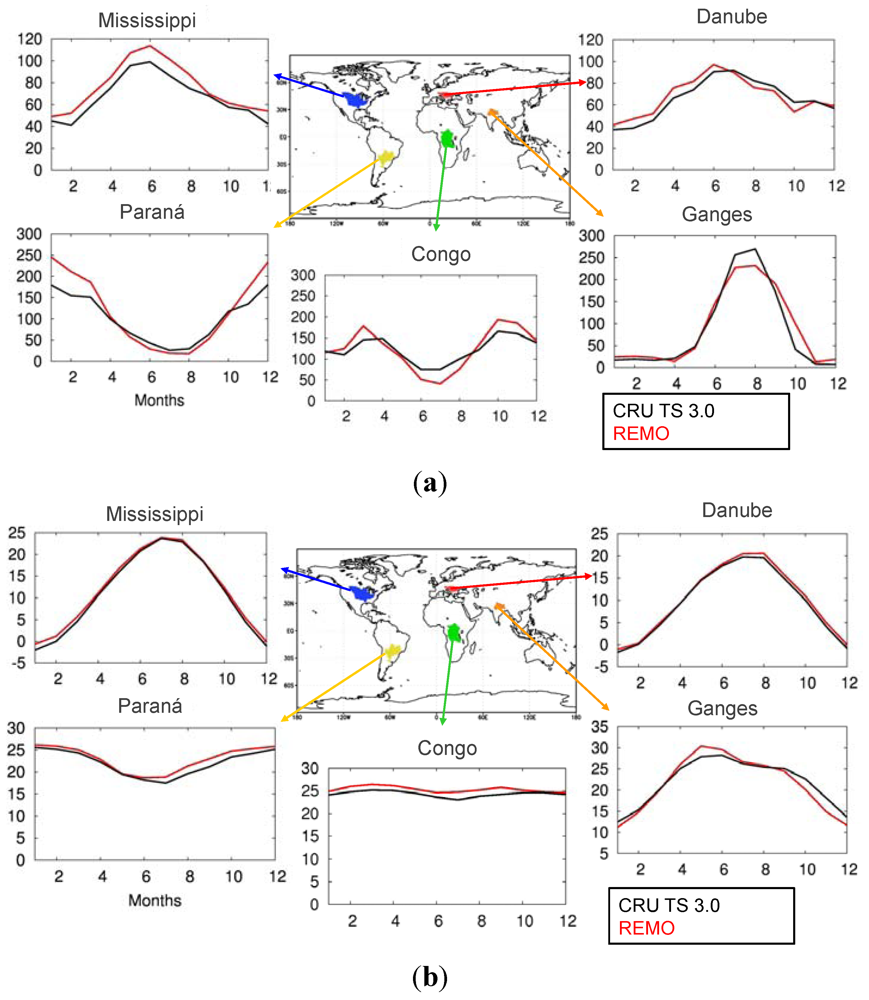
Figure 4 shows the annual cycles of precipitation and temperature for different river basins of each domain. It is evident from these figures that REMO has simulated the annual cycles of both the variables very well. Considering the fact that according to Köppen-Trewartha (Figure 2) these basins are situated in different climate types with the Congo being typically tropical, Paraná and Ganges being subtropical and Danube and Mississippi mainly having temperate climate, the model’s performance appears even more satisfactory. As shown in Figure 4(a), REMO has captured the dual maxima of precipitation of the Congo basin, which is associated with the annual movement of the Intertropical Convergence Zone (ITCZ). However the simulated seasonality over the Paraná Basin is larger than the corresponding observed seasonal cycle, with higher (less) amounts of precipitation during the rainy (dry) season. Over the west Asian domain, considering it is a “notoriously difficult to predict” nature of South Asian Summer Monsoon [35], REMO has captured the seasonality between wet and dry season quite well with a small dry and wet bias in monsoon and post monsoon months, respectively. Also for Danube and Mississippi river basins, the model results are very similar to observations with differences lower than 10 mm/month in each month for both basins. For the annual cycle of temperature (Figure 4(b)), it can be seen that model has captured the strong seasonality in the case of Danube, Mississippi and Ganges, and weak seasonality for the case of Congo and Paraná basins quite well. The maximum difference of around 2 °C occurs in a few months for Paraná and Ganges, however for other basins it remains within 1 °C difference.

Figure 4.
Annual cycles of (a) Precipitation [mm/month] (b) Temperature [°C] of selected catchments over each domain. Black and Red curves denote the CRU observations and REMO results respectively. The period considered is 1989 to 2006.
Figure 4.
Annual cycles of (a) Precipitation [mm/month] (b) Temperature [°C] of selected catchments over each domain. Black and Red curves denote the CRU observations and REMO results respectively. The period considered is 1989 to 2006.
4.2. Temperature Precipitation Relationship
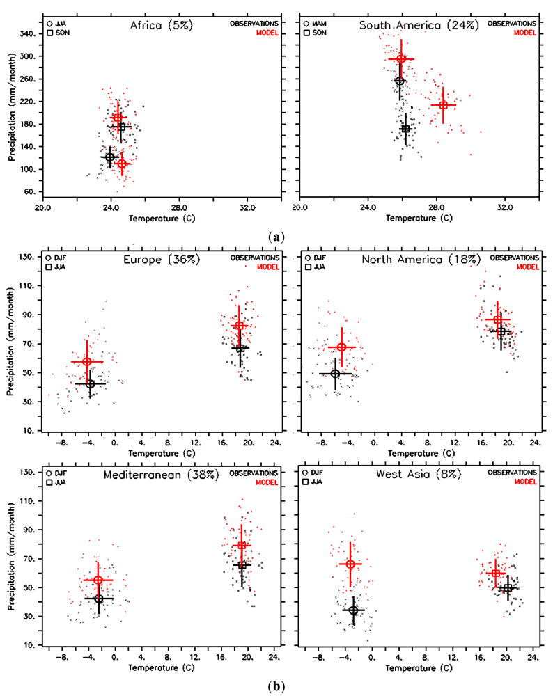
The precipitation-temperature relationship plots according to the Köppen-Trewartha climate classification types both for REMO and CRU data are discussed in this subsection. The area for each climate type is defined using Köppen-Trewartha climate classification based on CRU data as shown in Figure 2. This relationship is calculated for each domain and for each climate type. Figure 5 shows a subset of the results of monthly values for precipitation-temperature regimes in different regions during different seasons. The two climate types shown are the tropical humid climate (Ar, as listed in Figure 2) of South America and Africa (Figure 5(a)) and the temperate continental climate (Dc) of Europe, Mediterranean, North America and West Asia (Figure 5(b)). The seasons are selected relative to the maximum and minimum temperature values at each region.
The clusters of observational and model data explain the intraseasonal variability, and they are quantified by the standard deviation. These values are summarized for all climate types in Table 2. The clusters’ shape, given by the temperature and precipitation spread data, can be seen as a characteristic of the climate type. It varies along the seasons and regions, accordingly. As observed for the Dc climate type, which has similar characteristics with subtropical summer-wet (Cw) climate type, the subarctic continental (Ec) climate type and the tundra/highland climate type (FT) (not shown), the intraseasonal variability of temperature is larger in December, January, February (above 10 °C) than in the June, July, August season (approximately 4 °C). In the case of precipitation, climate types such as Ar (shown in Figure 5(a)) and the tropical wet-dry (Aw and As) climate type have values between 100 to 360 mm/month during rainy seasons. This variability is larger compared to the dry seasons of Aw, the dry semi-arid (Bs) climate type and the dry arid (Bw) climate type with monthly precipitation values between 10 to 40 mm/month. This is indicated as well by the standard deviation values at Table 2. The standard deviation from the model data is comparable to the observations for the climate type Dc, with the exception of the North American region. In general, the difference of the standard deviation values between the model and observational data is smaller at the climate types located in the midlatitudes than in the low and high latitudes.
Figure 5 also shows the interseasonal differences given by the differences in the precipitation-temperature regimes through the two seasons. This is expressed as two different clusters of data in each panel. The interseasonal differences for each climate type depends on several features at local, mesoscale and synoptic processes scales. In climate types representative of lower latitudes (e.g., Ar), small interseasonal differences for temperature (less than 1 °C) are observed. However, strong interseasonal changes in precipitation are observed where the range is between 60 to 100 mm/month (Figure 5(a)). Moving polewards, these interseasonal temperature changes become more noticeable such as in midlatitude climate types (e.g., Dc). Moving further towards the higher latitudes, these interseasonal temperature-precipitation differences become even larger with greater than 10 °C for temperature and 40 to 200 mm/month for precipitation (figure not shown). The differences on the regimes for the same climate type in different regions are a consequence of the climate type classification adopted in this study.
Köppen and Trewartha classification in comparison to other climate classification such as Köppen and Geiger [36] have established lower threshold values that define the climate types, and therefore bring together separated climate subtypes from Köppen and Geiger classification. The inversion of the warm or cold seasons (for climate types such as Aw, the subtropical humid (Cr) climate type and the temperate oceanic (Do) climate type) is a consequence of the geographical location situated on opposite hemispheres for that climate types.
Biases can be analyzed through the differences on the mean values. Reiterated bias appear on different climate types, high latitudes climate types such as Dc, Ec and FT show larger positive bias on precipitation compared to Ar. It is difficult to find a general attribution to this common bias. Misrepresentation of different processes could lead to the same signal model errors. Part of the bias on extreme climates like FT, could be attributed to the quality of the observation dataset as well. Over those areas, the dataset mainly presents two problems: low density of stations distribution and underestimation in instrument measurements due to the precipitation undercatch as a consequence of large wind speed. Temperatures in general are well represented, only larger biases around 2 °C are observed for tropical climate types (Ar and Aw) types, mainly at the Amazon region in South America. These biases, as explained in the previous section, take place during September, October, November months. At these latitudes, convection processes are very active and therefore the physical part of the model considered more difficult to reproduce than the dynamical part, might contribute to the biases.

Figure 5.
Seasonal Climate types Ar (a) and Dc (b). Each group of data represents observations and model results. Each dot represents the monthly mean value of precipitation and temperature in each month of the corresponding season. Seasons at each plot are identified by their different temperature-precipitation regime that results in two clusters of two groups of data. The seasons were chosen to represent the periods in which precipitation and/or temperature maximum and minimum values take place throughout the year, in this way, maximal annual amplitude is represented, note that the Ar climate type in Africa has two wet periods in the year (March, April, May and September, October, November), then June, July, August was selected as the dry season. The mean for both variables, temperature and precipitation, is represented by a square or a circle for each season. The bars represent the standard deviation. The percentage values correspond to the area covered by the climate type with respect to the total land area in the region. The period considered is 1989 to 2006.
4.3. PDF Skill Score
In this section, the results of the PDF skill score method are shown to evaluate the transferability of the model. Altogether there are 30 regions of different climate type and model domains on which the ranking of scores is based. Each skill score is calculated based on the comparison with CRU data in the same subregion. Using the climate classification types allows a quantitative measure of the model’s skill unlike previous studies wherein model results are subdivided according to unphysical criteria such as administrative borders or regular boxes [7].
The continents are subdivided into different regions according to climate types. In regions with the same climate type, the characteristics in precipitation and temperature distributions are alike. For instance, in continental temperate climate (Dc) regions in Europe (Figure 6(a)), the temperature distribution based on the gridded observational dataset, tends to be bimodal. The maximum probabilities are at around 0 and 20 °C. The observed extreme monthly mean precipitation values can reach up to 700 mm/month. In domains with this climate type (Europe, Mediterranean, West Asia, and North America), the model represents well the bimodality of the temperature distribution and thus has high skill scores (more than 0.9). However the model overestimates the occurrence of high values of monthly mean precipitation. The good representation of the more frequent but lower precipitation rates still leads to a high skill score (more than 0.8).
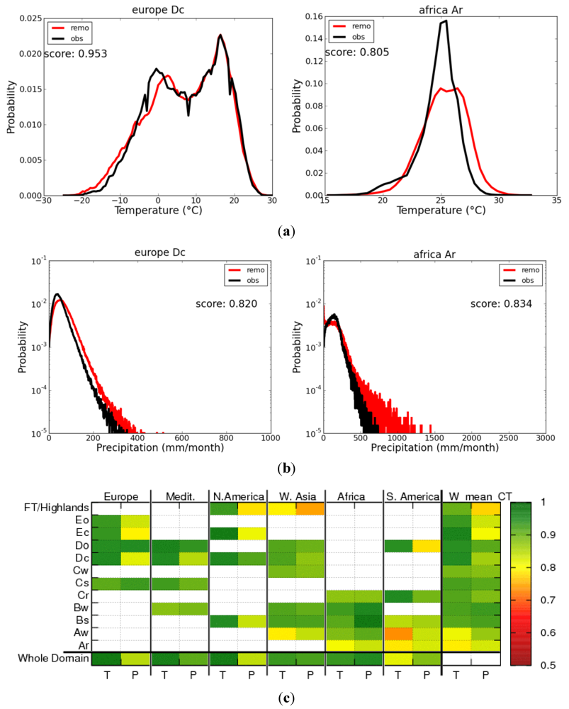
Figure 6.
Probability density function (PDF) Skill scores for (a) temperature (T) and (b) precipitation (P). Example PDF results in selected regions: temperate continental climate (Dc) over Europe (a and b, left); and tropical humid climate (Ar) over Africa (a and b, right). The temperature and precipitation PDF curves for the observed (black) and simulated (red) distributions are shown. The precipitation plots are in logarithmic scale and the probability values shown are equal or greater than 10−5. (c) Summary of the PDF skill scores for all climate types. The last column shows the weighted mean of PDF skill scores (W_mean_CT) across different domains for every climate type. The period considered is 1989 to 2006.

In contrast to the relatively high skill score in the temperate climate region discussed above, relatively low skill scores especially in temperature can be found in regions with the tropical humid climate type (Ar) in Africa and South America (Figure 6(b)). The observations show a unimodal temperature distribution which peaks at around 25 °C. The distribution of the simulated monthly mean temperature values shows a similar behavior but underestimates their frequency between 24 °C and 28 °C. In addition, the model also simulates higher probabilities for temperature values of more than 27 °C. This can also be seen in Section 4.1, where the warm bias of the model in comparison with CRU data can be observed.
Skill scores for all climate types and all regions are summarized in the table in Figure 6(c). High skill scores (relative to the whole table) are represented in green, while lower skill scores are represented in red. In general it can be seen that for temperature, skill scores are higher for the more temperate climate types than for the more extreme climate types such as tundra (FT), tropical wet-dry (Aw) and tropical humid (Ar). For precipitation a similar behavior can be observed. High skill scores in precipitation are found in temperate climates except for the temperate oceanic (Do) climate type in South America. In regions with low skill score, the model tends to simulate higher precipitation rates and higher occurrence of these rates compared to CRU data.
The last row and the last column in Figure 6(c) represent the overall skill of REMO for all domains and climate types, respectively. The skill of the model in each domain is calculated using all monthly precipitation and temperature values disregarding the climate types. In evaluating the skill of the model according to the different climate types, the PDF skill score is calculated using the weighted mean of climate types’ scores at different domains. In this figure, the performance of REMO for temperature is best in the European, Mediterranean and North American domain, while it is comparatively low in South America. Precipitation shows highest skill scores for the Mediterranean, African and West Asian regions.
The scores for temperature are high in the midlatitude climate types and the lowest are in the tropical climate types (Ar, Aw). In the case of precipitation, skill scores are lowest for arctic and tundra/highland climate types. The other climate types are simulated well by the model.
5. Conclusions
The regional climate model REMO has been applied for hindcast simulations over 6 CORDEX regions (Africa, Europe, Mediterranean, North America, South America and West Asia) using the same model parameters and parameterizations for all domains for the years 1989–2008. A new framework has also been introduced which accounts, not only for mean annual climate features and annual cycles of precipitation and temperature, but also considers inter- and intra-seasonal characteristics as well as representing these variables based on probability density functions against observations. A comparison to CRU observational estimates of precipitation and temperature has shown that REMO is able to simulate the mean annual climatic features in all domains quite reasonably. The model has also performed well in capturing the annual cycle of precipitation and temperature over selected catchments out of each domain. Considering the different climatic characteristics of these catchments, the performance of the model looks even more impressive.
From the analysis of precipitation-temperature relationship plots based on the Köppen-Trewartha climate classification [6], it is found that in general the model is able to catch the inter- and intra-seasonal variability for most of the climate classes. Moreover, the model has successfully simulated the small inter-seasonal differences for temperature and precipitation for lower latitudes, which increase further and further while moving towards the higher latitudes. From the PDF skill score method, it is found that REMO is capable of representing the characteristics of the Köppen-Trewartha climate types over the six chosen domains. In this study, the skill scores range from 0.7 to 0.9. These values are not directly comparable with the skill scores derived in Perkins et al. [7], which range between 0.5 and 0.8. Skill score values in Perkins et al. [7] are based on daily datasets for Australia which are aggregated by different regions instead of monthly data aggregated for different climate types. However, the high skill scores for the case of REMO again speak for the effectiveness of REMO over the simulated regions.
There are, however, some regions in which the simulation results show less accuracy, e.g., in the region of the Ar climate type in South America. During the course of the study, the prominent biases originating from the above-mentioned evaluation strategy have been pointed out and the probable reasons for each of them have been discussed. For some biases, the reason seems to be the non- or mis-representation of some processes in the model. For example, the systematic warm biases near the coast of major upwelling regions may be attributed to the misrepresentation of the processes of the stratocumulus clouds or to a missing air-sea interaction in the local atmosphere due to the prescribed SST. However, for some other biases, the inability of observations to correctly represent the climate of the regions seems to be the problem. One example is the significant overestimations of precipitation over mountain chains at high altitude which may be attributed to the scarce data availability and the missing undercatch correction in the CRU data.
In contrast to the findings of Takle et al. [4], the reasonably good performance of the unmodified REMO model in regions representing a large spectrum of climate types, gives confidence in the representation of the meteorological processes in the model under different climatic conditions. This finding is especially important for assessing future climate projections, as climate conditions might also change in the future. Even though REMO seems to perform best over its home domain of Europe, its simulated climate is not significantly worse over the other domains. Thus, the evaluation of the ERA Interim driven simulations has shown that REMO is suited well for climate change simulations over each of the six presented CORDEX regions. These simulations will provide very useful information about the regional climate change characteristics, which then can further be used in regional climate change impact and adaptation studies.
In addition to the domains considered in the present study, further REMO simulations are currently in progress, such as a very high resolution (about 12 km) simulation over Europe and a coupled atmosphere-ocean simulation over the Mediterranean. It is planned to assess the performance of REMO using additional observational datasets, which are more detailed in specific regions. This will also give an estimate of the quality of the global gridded observational CRU dataset in these regions.
Acknowledgments
REMO simulations for West Asia, South America and Mediterranean were conducted under various projects such as HighNoon (FP7 Grant Agreement No. 227087), CLARIS-LPB (FP7 Grant Agreement No. 212492), CIRCE (FP6 Grant Agreement No. 036961), respectively. The REMO simulations for the other domains were performed under the “Konsortial” share at the German Climate Computing Centre (DKRZ), which we are further thankful for their various support.
References
- WCRP CORDEX. Available online: http://wcrp.ipsl.jussieu.fr/SF_RCD_CORDEX.html (accessed on 20 October 2010).
- Jacob, D.; Barring, L.; Christensen, O.B.; Christensen, J.H.; de Castro, M.; Deque, M.; Giorgi, F.; Hagemann, S.; Lenderink, G.; Rockel, B.; et al. An inter-comparison of regional climate models for Europe: Model performance in present-day climate. Clim. Change 2007, 81, 31–52. [Google Scholar] [CrossRef]
- Simmons, A.; Uppala, S.; Dee, D.; Kobayashi, S. ERA-Interim: New ECMWF reanalysis products from 1989 onwards. ECMWF Newslett. 2006, 110, 25–35. [Google Scholar]
- Takle, E.S.; Roads, J.; Rockel, B.; Gutowski, W.J., Jr.; Arrit, R.W.; Meinke, I.; Jones, C.G.; Zadra, A. Transferability intercomparison: An opportunity for new insight on the global watercycle and energy budget. Bull. Am. Meteor. Soc. 2007, 88, 375–384. [Google Scholar] [CrossRef]
- Jacob, D.; Podzun, R. Sensitivity studies with the regional climate model REMO. Meteorol. Atmos. Phys. 1997, 63, 119–129. [Google Scholar] [CrossRef]
- Trewatha, G.T. An Introduction to Climate, 3rd ed; McGraw-Hill: New York, NY, USA, 1954. [Google Scholar]
- Perkins, S.E.; Pitman, A.J.; Holbrook, N.J.; McAneney, J. Evaluation of the AR4 climate model’s simulated daily maximum temperature, minimum temperature, and precipitation over Australia using probability density functions. J. Climate 2007, 20, 4356–4376. [Google Scholar] [CrossRef]
- Jacob, D. A note to the simulation of the annual and inter-annual variability of the water budget over the Baltic Sea drainage basin. Meteorol. Atmos. Phys. 2001, 77, 61–73. [Google Scholar] [CrossRef]
- Roeckner, E.; Arpe, K.; Bengtsson, L.; Christoph, M.; Claussen, M.; Dümenil, L.; Esch, M.; Giorgetta, M.; Schlese, U.; Schulzweida, U. The Atmospheric General Circulation Model Echam-4: Model Description and Simulation of the Present Day Climate; Report No. 218; Max-Planck-Institute for Meteorology: Hamburg, Germany, 1996. [Google Scholar]
- Majewski, D. The Europa-Modell of the Deutscher Wetterdienst. In Proceedings of the ECMWF Seminar on Numerical Methods in Atmospheric Models, Reading, UK, 9–13 September 1991; pp. 147–191.
- Tiedtke, M. A comprehensive mass flux scheme for cumulus parameterization in large scale models. Mon. Weather Rev. 1989, 117, 1779–1800. [Google Scholar] [CrossRef]
- Nordeng, T.E. Extended Versions of the Convective Parametrization Scheme at ECMWF and Their Impact on the Mean and Transient Activity of the Model in the Tropics; Technical Report No. 206; European Centre for Medium-Range Weather Forecasts: Reading, UK, 1994. [Google Scholar]
- Pfeifer, S. Modeling Cold Cloud Processes with the Regional Climate Model Remo; Reports on Earth System Science 23; Max-Planck-Institute for Meteorology: Hamburg, Germany, 2006. [Google Scholar]
- Morcrette, J.J.; Smith, L.; Fourquart, Y. Pressure and temperature dependance of the absorption in longwave radiation parameterizations. Beitr. Phys. Atmos. 1986, 59, 455–469. [Google Scholar]
- Giorgetta, M.; Wild, M. The Water Vapour Continuum and Its Representation in Echam4; Report No. 162; Max-Planck-Institute for Meteorology: Hamburg, Germany, 1995. [Google Scholar]
- Louis, J.F. A parametric model of vertical eddy fluxes in the atmosphere. Bound. Layer Meteorol. 1979, 17, 187–202. [Google Scholar] [CrossRef]
- Lohmann, U.; Roeckner, E. Design and performance of a new cloud microphysics scheme developed for the ECHAM4 general circulation model. Clim. Dyn. 1996, 12, 557–572. [Google Scholar] [CrossRef]
- Hagemann, S. An Improved Land Surface Parameter Dataset for Global and Regional Climate Models; Report No. 336; Max-Planck-Institute for Meteorology: Hamburg, Germany, 2002. [Google Scholar]
- Rechid, D.; Raddatz, T.J.; Jacob, D. Parameterization of snow-free land surface albedo as a function of vegetation phenology based on MODIS data and applied in climate modelling. Theor. Appl. Climatol. 2009, 95, 245–255. [Google Scholar] [CrossRef]
- Davies, H.C. A lateral boundary formulation for multi-level prediction models. Quart. J. R. Meteor. Soc. 1976, 102, 405–418. [Google Scholar]
- CRU Datasets-CRU TS Time-Series; British Atmospheric Data Centre: Didcot, UK, 2008. Available online: http://badc.nerc.ac.uk/view/badc.nerc.ac.uk__ATOM__dataent_1256223773328276 (accessed on 20 October 2010).
- Brohan, P.; Kennedy, J.J.; Harris, I.; Tett, S.F.B.; Jones, P.D. Uncertainty estimates in regional and global observed temperature changes: A new dataset from 1850. J. Geophys. Res. 2006, 111. [Google Scholar]
- Legates, D.R.; Willmott, C.J. Mean seasonal and spatial variability in gauge-corrected, global precipitation. Int. J. Climatol. 1990, 10, 111–127. [Google Scholar] [CrossRef]
- Lohmann, U.; Sausen, R.; Bengtsson, L.; Cubasch, U.; Perlwitz, J.; Roeckner, E. The Köppen climate classification as a diagnostic tool for general circulation models. Clim. Res. 1993, 3, 177–193. [Google Scholar] [CrossRef]
- de Castro, M.; Gallardo, C.; Jylha, K.; Tuomenvirta, H. The use of a climate-type classification for assessing climate change effects in Europe from an ensemble of nine regional climate models. Clim. Change 2007, 81, 329–341. [Google Scholar] [CrossRef]
- Tapiador, F.J.; Sánchez, E.; Romera, R. Exploiting an ensemble of regional climate models to provide robust estimates of projected changes in monthly temperature and precipitation probability distribution functions. Tellus A 2009, 61, 57–71. [Google Scholar] [CrossRef]
- Kleidon, A.; Heimann, M. Assessing the role of deep rooted vegetation in the climate system with model simulations: Mechanism, comparison to observations and implications for Amazonian deforestation. Clim. Dyn. 2000, 16, 183–199. [Google Scholar] [CrossRef]
- Haensler, A.; Hagemann, S.; Jacob, D. Dynamical downscaling of ERA40 reanalysis data over southern Africa: Added value in the representation of seasonal rainfall characteristics. Int. J. Climatol. 2011, 31, 2338–2349. [Google Scholar] [CrossRef]
- Richter, I.; Mechoso, C.R. Orographic influences on subtropical stratocumulus. J. Atmos. Sci. 2006, 63, 2585–2601. [Google Scholar] [CrossRef]
- Yu, J.-Y.; Mechoso, C.R. Links between annual variations of peruvian stratocumulus clouds and of SST in the Eastern Equatorial Pacific. J. Clim. 1999, 12, 3305–3318. [Google Scholar]
- Yang, D.; Kane, D.; Zhang, Z.; Legates, D.; Goodison, B. Bias corrections of long-term (1973-2004) daily precipitation data over the northern regions. Geophys. Res. Lett. 2005, 32. [Google Scholar]
- Dai, A.; Qian, T.; Trenberth, K.E.; Milliman, J.D. Changes in continental freshwater discharge from 1948 to 2004. J. Clim. 2009, 22, 2773–2791. [Google Scholar] [CrossRef]
- Dai, A.; Trenberth, K.E. Estimates of freshwater discharge from continents: Latitudinal and seasonal variations. J. Hydrometeor. 2002, 3, 660–687. [Google Scholar] [CrossRef]
- Hagemann, S.; Duemenil, L. A parameterization of the lateral waterflow for the global scale. Clim. Dyn. 1998, 14, 17–31. [Google Scholar] [CrossRef]
- Jayaraman, K.S. Rival monsoon forecasts banned. Nature 2005, 436. [Google Scholar]
- Kottek, M.; Grieser, J.; Beck, C.; Rudolf, B.; Rubel, F. World map of the Köppen-Geiger climate classification updated. Meteorol. Z. 2006, 15, 259–263. [Google Scholar] [CrossRef]
© 2012 by the authors; licensee MDPI, Basel, Switzerland. This article is an open-access article distributed under the terms and conditions of the Creative Commons Attribution license (http://creativecommons.org/licenses/by/3.0/).