Review

Numerical Modeling of Climate-Chemistry Connections: Recent Developments and Future Challenges

Institute of Atmospheric Physics, German Aerospace Center, Oberpfaffenhofen, D-82234 Wessling, Germany
*
Author to whom correspondence should be addressed.
Atmosphere 2013, 4(2), 132-156; https://doi.org/10.3390/atmos4020132
Submission received: 26 March 2013 / Revised: 3 May 2013 / Accepted: 8 May 2013 / Published: 17 May 2013
(This article belongs to the Special Issue Ozone Depletion and Climate Change)

Abstract

:
This paper reviews the current state and development of different numerical model classes that are used to simulate the global atmospheric system, particularly Earth’s climate and climate-chemistry connections. The focus is on Chemistry-Climate Models. In general, these serve to examine dynamical and chemical processes in the Earth atmosphere, their feedback, and interaction with climate. Such models have been established as helpful tools in addition to analyses of observational data. Definitions of the global model classes are given and their capabilities as well as weaknesses are discussed. Examples of scientific studies indicate how numerical exercises contribute to an improved understanding of atmospheric behavior. There, the focus is on synergistic investigations combining observations and model results. The possible future developments and challenges are presented, not only from the scientific point of view but also regarding the computer technology and respective consequences for numerical modeling of atmospheric processes. In the future, a stronger cross-linkage of subject-specific scientists is necessary, to tackle the looming challenges. It should link the specialist discipline and applied computer science.

1. Introduction

Numerical models are widely used for investigations of atmospheric conditions and behavior. Their results are combined with analyses from atmospheric observations, for instance those representing the chemical composition, the thermal, or the dynamical structure of Earth’s atmosphere. A major goal of atmospheric numerical modeling is to provide a better understanding of processes determining the dynamical and chemical state, and to enable assignment of individual natural and anthropogenic forces, which are relevant for the variability and long-term change of atmospheric quantities. Processes on different spatial and temporal scales are studied determining the status and temporal evolution of the atmosphere. Such “atmospheric models” allow the evaluation of specific processes as well as feedback mechanisms, in particular the disclosure of cause-effect-chains. Last but not least, improving numerical models enhances the skill of weather forecasts and projections of future climate change. Understanding weaknesses by confronting hindcasts with observations generates the expert knowledge required to judge model performance.
In recent years, numerical investigations of changes in atmospheric behavior due to natural and anthropogenic factors have played an increasing role in atmospheric sciences. For instance, numerical modeling supports the attribution of specific causes for spatial and temporal variability, changes, or trends of atmospheric conditions. Model based examination of dynamical, chemical, and radiative processes and their interactions, ranks equally to analyses of in situ or remote sensing measurements; it is a cornerstone of atmospheric research. Numerical models are useful tools to explain observed processes (e.g., by testing hypotheses). Therefore, atmospheric models are an integrating part between observations and our theoretical understanding of processes. Prominent examples, demonstrating the important role of numerical modeling in atmospheric and climate research, are the highly recognized 4th Assessment Report of the Intergovernmental Panel on Climate Change [1] and the WMO/UNEP Scientific Assessment of Ozone Depletion: 2010 [2]. In these assessments, general conclusions with respect to climate change and climate-chemistry interactions were based to a large degree on results derived from numerical model simulations. Both assessment reports have demonstrated that it is a challenge to interpret atmospheric variability and climate change on different spatial and temporal scales.
Scientific progress can be achieved by analyzing a broad set of model simulations and subsequent evaluation of model results with respective observations. A detailed confrontation of data products derived from measurements and model simulations is a crucial task: It helps to identify strengths and weaknesses of the applied model systems in explaining the recent evolution of the atmosphere and climate; it encourages disclosing insufficient knowledge of individual atmospheric processes and the feedback between different processes, which is necessary for adequate further developments and improvements of the atmospheric models.
For instance, investigations of climate change and climate-chemistry interactions are based on the synergistic use of data derived from observations and those from respective model simulations [3]. So-called hindcast simulations aim at reproducing past atmospheric conditions. In combination with detailed analyses of observational data sets, numerical models are used to separate single processes and to assess their roles for the whole climate system. Moreover, numerical studies enable a detailed investigation of interactions of dynamical and chemical processes in Earth’s atmosphere; they allow an evaluation of the role of the Middle Atmosphere (atmospheric layers above the troposphere, which include the stratosphere from about 12 to 50 km, and the mesosphere from 50 to 100 km) for climate change. Finally, the interplay of the atmosphere with oceans, the cryosphere, and the biosphere have been investigated with “coupled” model systems, i.e., atmospheric models interactively linked to respective model systems.
A better understanding of mechanisms can be gained if sensitivity simulations are performed in addition to a reference simulation; they allow attribution of causes to particular atmospheric behavior. In this case, specific assumptions or boundary conditions are modified and the subsequent consequences are quantified. Moreover, the role of parameterizations can be studied describing sub-grid-scale processes (see below): for example, investigations using alternative parameterizations characterizing the same single process help to assess uncertainties and how these affect the whole system. Evaluated model systems that are able to reproduce main features like the mean state or long- and short-term variability of important dynamic or chemical quantities are used to perform sets of scenario simulations. They form the basis for assessments of the future evolution of atmospheric dynamics and chemistry following specific scenarios, including the specification of uncertainties. In doing so, specified (boundary) conditions are adopted for the future. Politicians are often using such future projections as basis for decisions regarding adaptation and mitigation strategies. This underlines the necessity of scientifically robust assessments, based on a solid knowledge and a serious evaluation of consequences. A prominent example in recent years, emphasizing the responsibility of atmospheric sciences, is the growing discussion about possibilities moderating global warming (caused by enhanced greenhouse gas concentrations), for example by cooling down Earth's climate by sulfur emissions in the stratosphere [4,5,6]. The concept of geo-engineering or climate engineering refers to the deliberate large-scale intervention in the Earth’s climate system, in order to slow-down climate change. It is the task of atmospheric scientists to provide reliable estimates of possible effects and further consequences on a serious basis.
This paper is focusing on global models currently used to study Earth’s atmosphere processes and climate. The next section provides a summary of the most common classes of global atmospheric models, so far used to investigate processes on planetary scale and on longer time scales, i.e., years to decades; capabilities and achievements are discussed. Section 3 gives some examples of actual atmospheric research topics and the particular contribution of exercises with Chemistry-Climate Models. Expected future developments in numerical modeling and challenges are discussed in Section 4, in particular the expected further improvements of computer technologies and consequences for numerical modeling of the atmosphere. The last section gives some general conclusions.

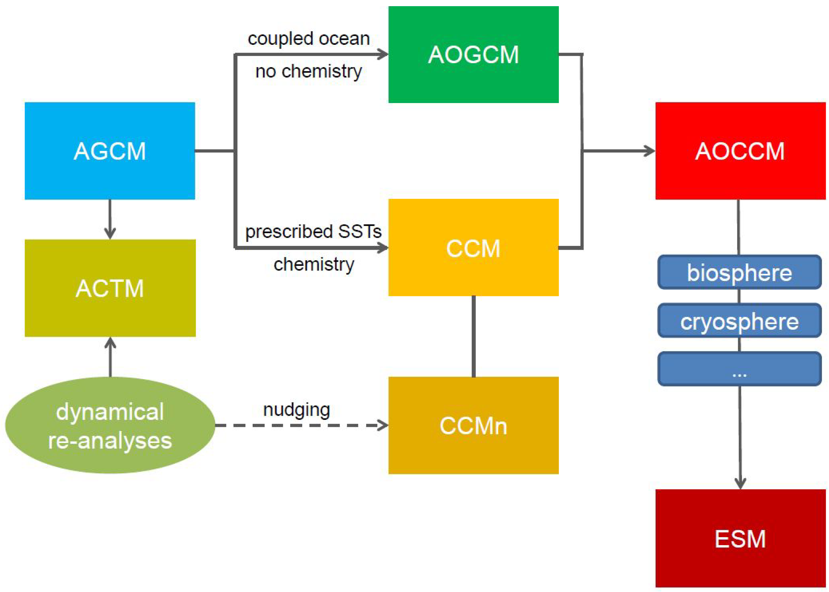
2. Global Atmospheric Model Systems

2.1. Definitions

In recent years investigations of atmospheric processes on global scale have mostly been based on three-dimensional (3-D) model systems, which are briefly described here. Figure 1 shows a schematic overview.
Figure 1. Schematic of global model systems to study climate change and climate-chemistry connections. AGCM: Atmospheric General Circulation Model; ACTM: Atmospheric Chemistry Transport Model; AOGCM: Atmosphere-Ocean General Circulation Model = global climate model; CCM: Chemistry-Climate Model; CCMn: “nudged” CCM; AOCCM: Atmosphere-Ocean Chemistry-Climate Model = global climate model with interactive chemistry; ESM: Earth-System Model. See text for detailed descriptions.
Atmosphere 04 00132 g001

2.1.1. Atmospheric General Circulation Model (AGCM)

This 3-D model type focuses on studying physical, radiative, and dynamical processes in the atmosphere on large spatial (a few hundred km) and temporal (over years and decades) scales. An AGCM is an “atmosphere only” model in which impacts of other, adjacent influencing factors are considered by boundary conditions (e.g., prescribed values) or due to parameterizations. For instance, sea surface temperatures (SSTs) and sea ice content (SIC) are predefined according to observations or values provided by ocean models. Concentrations of radiatively active gases (greenhouse gases like carbon dioxide (CO2), methane (CH4), nitrous oxide (N2O), chlorofluorocarbons (CFCs), and ozone (O3)) and aerosols are predefined based on measurements or given scenarios, since chemical processes are usually not taken into account in numerical simulations with AGCMs. Changes of water vapor (H2O) concentrations due to the hydrological cycle are typically directly simulated by an AGCM.

2.1.2. Atmosphere-Ocean General Circulation Model (AOGCM)

An AGCM interactively coupled to an ocean model, commonly referred to as an Atmosphere-Ocean General Circulation Model (AOGCM) or a global climate model, is used for investigations of climate change. Ozone fields are mostly prescribed without considering feedbacks (e.g., climate-ozone connections) and effects of chemical processes on water vapor are neglected. In AGCMs and AOGCMs, the impact of human activities is generally considered by prescribing mixing ratios of long-lived (well-mixed) greenhouse gases (i.e., CO2, CH4, and N2O), anthropogenic aerosol, and radiatively active ozone depleting substances (ODSs: CFCs, halogenated CFCs (HCFCs), and halons). Natural forcing such as changes in solar activity and volcanic eruptions are also taken into account by prescribed boundary conditions.

2.1.3. Atmospheric Chemistry Transport Model (ACTM)

In these models, simulations of chemical processes and transport of trace gases and particles (aerosols) in the atmosphere use prescribed dynamical fields; they are either derived from observations (e.g., meteorological re-analyses, which are usually based on numerical weather prediction (NWP) models using data assimilation schemes), or AGCM output (e.g., calculated values for specific conditions or projected values for the future). In particular, an ACTM uses winds and temperatures to calculate the atmospheric transport and the abundances of chemical species. ACTMs can share with AGCMs a common advection scheme. ACTMs do not consider the feedback of the chemical composition of the atmosphere to dynamics via radiative processes; they are “non-interactive” models. Furthermore, they are used to simulate the temporal evolution of atmospheric composition and help interpret observations.

2.1.4. Chemistry-Climate Model (CCM)

If an AGCM is interactively coupled to a chemistry model it is called Chemistry-Climate Model (CCM). This naming can be misleading since SSTs and SIC are most often prescribed, and the atmospheric model part is not interactively coupled to an ocean model as in a global climate model (AOGCM). In a CCM, simulated concentrations of radiatively active gases are used in the calculations of heating and cooling rates. Changes in the abundance of these gases due to chemistry and advection directly influence net heating rates (i.e., the sum of heating and cooling rates) and, consequently, affect variables that describe atmospheric dynamics such as temperature, pressure, and wind. In this context, the impact of aerosols (e.g., after large volcanic eruptions) is also considered, both in the treatment of chemical and radiative processes. Another feedback to be considered is via the hydrological cycle including formation and sublimation of clouds (e.g., polar stratospheric clouds, PSCs). This gives rise to a dynamical-chemical coupling in which the chemistry influences the dynamics via radiative heating changes and vice versa via temperature and advection. In contrast to an ACTM, a CCM is an “interactive” model. Not all of the CCMs have full coupling for all chemical constituents; some radiatively active gases are specified in either the radiation or chemistry modules. Typically ozone and water vapor are fully coupled, as they represent the prevailing radiative-chemical feedback in the atmosphere, especially in the stratosphere. Changes in the amount and distribution of water vapor and ozone are calculated in a self-consistent manner considering interactions of chemical, radiative, and dynamical (transport and mixing) processes. In recent years, CCMs have been key tools for the attribution and projection of the response of stratospheric ozone to ozone depleting substances (ODSs) like CFCs and other factors.
Sometimes, dynamical quantities in a CCM are relaxed towards observations for a direct comparison of CCM results with observations of chemical quantities. In these so-called “nudged CCMs” (in the following abbreviated CCMn) a non-physical correction term is introduced in the model equations for prognostic variables like divergence, vorticity, wind, (potential) temperature, or surface pressure to steer the model dynamics towards the observed meteorology. The nudging terms are defined as the difference between the observation and the model solution weighted by nudging coefficients, which are actually relaxation times [7]. In other words, nudging provides a weak correction of the calculated tendencies of the prognostic variables.

2.1.5. On-Going Developments

At present there are extensive efforts building up global climate models with interactive chemistry, by either coupling a chemistry code to an AOGCM or coupling an ocean model to a CCM. Theses model systems, in the following named AOCCMs (Atmosphere-Ocean Chemistry-Climate Models), are more consistent regarding the assessment of interactions between climate change and atmospheric chemistry. Regarding the coupling of atmospheric and oceanic processes one has to distinguish between dynamical and chemical coupling. So far the coupling was mostly limited to the dynamical component, neglecting the exchange of reactive gases between the atmosphere and the ocean. In any case, it is not enough to simply couple models representing different sub-systems, but after coupling the domain models, the global annual mean radiation balance of the “coupled” model system has to be adjusted; otherwise significant biases can be introduced.
In the last decade, CCMs have often been used for investigations related to the stratospheric ozone layer [3]; the chemistry modules implemented in those CCMs are simplified because they mostly represent only stratospheric homogeneous and heterogeneous ozone chemistry and the most relevant chemical processes for describing the tropospheric background chemistry. A step forward is therefore the inclusion of more detailed tropospheric chemistry in these CCMs (e.g., considering the non-methane hydrocarbon chemistry); more complex “tropospheric” CCMs are already available and have been, for example, used in connection with investigations related to CMIP (Coupled Model Intercomparison Project; see below) activities. Full chemistry, either in CCMs or AOCCMs, allows more detailed investigations of the interaction of tropospheric and stratospheric chemistry in a changing climate [8]. As a consequence, not only a higher vertical resolution of the upper troposphere/lower stratosphere (UTLS) region is required (nowadays in the order of 1–2 km), but also an enhanced horizontal resolution is necessary (currently about 2–3 degrees latitude/longitude) for an adequate treatment of the dynamical and chemical coupling of the troposphere and the stratosphere including the exchange of air masses. Beyond that, studies of feedbacks between climate change and variations and trends of atmospheric composition will be set on a more consolidated basis.
The majority of currently available AOGCMs and CCMs consider the entire troposphere, the whole stratosphere, but only parts of the mesosphere (mostly up to about 80 km). The consideration of at least the whole mesosphere (up to 100 km) is envisaged since there are strong hints that it is plays an important role in climate change [9,10,11]. It might also be necessary to consider the lower part of the thermosphere (approximately up to 120 km) to describe the mesopause region in a sufficiently detailed way.
At the moment, diverse efforts aim at considering additional feedback processes in AOGCMs or AOCCMs. These are, for instance, related to the carbon cycle, to the interaction with the biosphere, the cryosphere, and the land surfaces; such models are called Earth-System Models (ESMs). This model type is meant to put together our knowledge regarding the coupling between physical and biogeo-chemical processes. A discussion about challenges, possibilities, and limitations establishing such complex model systems including the requirements on high-performance computing is given in Section 4.

2.2. Capabilities and Limitations

At present, the different atmospheric models mentioned above represent a backbone of numerical climate research on global scale. They all have obvious strengths and weaknesses and are applied for specific issues. In the following, a brief overview is given about fields of application and limitations.
AGCMs are suitable tools to examine dynamical processes (e.g., large scale wave-mean flow interactions) under different climate conditions. The origin of short- and long-term variability can be studied as well as the reasons for changes and trends in atmospheric circulation. Among others, current investigations are focusing on the Brewer-Dobson circulation and its possible change in a future climate (Chapter 4 in [3]) [12,13,14]. The circulation is important for transport and hence the distribution of trace substances in the stratosphere. In this context, advanced knowledge can be obtained, e.g., by comparing results derived from AGCM simulations with fixed boundary conditions representing particular mean climate states, i.e., so-called time slice simulations: Here, the internal variability of an AGCM can be investigated under invariant conditions, e.g., for greenhouse gas concentrations, SSTs and SIC, to assess the statistical significance of specific changes. A disadvantage of an AGCM is that it does not consider interactions with atmospheric chemistry, suppressing the feedback of dynamical and chemical processes. Another restriction is that this kind of model system focuses on planetary and synoptic scales of a few hundred kilometers. Sub-grid-scale processes, like effects of unresolved atmospheric waves (e.g., gravity waves) or clouds, have to be parameterized because of insufficient resolution of the used models. For example, one of the most challenging aspects of modeling the dynamical coupling of the troposphere and stratosphere is the parameterization of orographic and non-orographic gravity waves and their feedback on the resolved flow. Parameterizations of increasing complexity are being developed to represent the dynamics of these waves more realistically. The free parameters are used to reproduce present-day climate. This raises a credibility issue when these gravity-wave parameterizations are employed for the purpose of climate change simulations. On the other hand it must be mentioned that high resolution global climate modeling is under way making some of these parameterizations eventually unnecessary.
Global climate models (AOGCMs) are basic numerical instruments for investigations of recent climate change and projections of possible future developments [15]. Typically, such models are used for multi-decadal simulations with variable boundary conditions, i.e., so-called transient simulations: Such simulations consider observed or predicted gradual changes in concentrations of radiatively active gases and other boundary conditions (e.g., tropospheric and stratospheric aerosol loading for a specific episode). To establish robust assessments of future conditions, the strategy is to run several independent global climate models from different research groups with the same (or at least very similar) boundary assumptions. Then, the differences between individual model results for a specific scenario can be gathered as an uncertainty range for the occurrence of a certain event. In this way, multi-model means are sometimes used as “the best estimate”. But this practice requires clear rules; it is questionable and implies strong limitations, if no performance requirements for the used models are defined in advance [16]. Another approach is similar to numerical weather prediction: a model is used for multiple simulations with slightly modified initial conditions, creating the most likely weather condition in a statistical sense. Even for global climate models, handling sub-grid-scale processes by using parameterizations is a non-negligible problem. In particular, the treatment of clouds and convective processes poses a huge unresolved problem (Chapter 2 in [1]. As for an AGCM, another constraint is the neglect of atmospheric chemistry. For example, in the past, many global climate models (AOGCMs) have invariant stratospheric ozone concentrations and did not consider ozone depletion in the second half of the last century and the expected recovery in the present century; consequently the cooling trend in the lower stratosphere has been clearly underestimated (Chapter 7 in [1], Chapter 4 in [2]) (see also Section 3.2).
ACTMs are the most common numerical methods to support field campaigns (or individual measurements), that focuses on observations of chemical quantities. On the one hand, implementing forecast data in an ACTM can help optimizing the measurement strategy in advance. On the other hand using re-analysis data provides a comprehensive data set helping to interpret the measured data in a broader context. Universally, ACTMs are used for investigations of particular chemical processes under controlled dynamical conditions. Sensitivity studies regarding specific prescribed dynamical values like temperature support investigations of separate processes: For example, the contributions of individual processes on changes in the chemical composition of the atmosphere caused by steady warming or cooling was quantified [17,18,19]. Neglecting dynamical-chemical feedback mechanisms is an obvious limitation if such a model system is used for assessments with respect to climate change consequences.
CCMs are self-consistent “atmosphere-only” models where the coupling of dynamical and chemical processes is handled interactively. Among others, in recent years this model type has been used in connection with questions regarding feedbacks of climate change and atmospheric chemistry, for instance the depletion and recovery of the stratospheric ozone layer [1,20] (see Section 3.2). Similarly to prognostic studies performed with global climate models, CCMs are also used for assessments of future atmospheric composition and dynamics: In this context CCMs are used for time-slice (i.e., with invariant boundary conditions representing a specific year) as well as transient (i.e., variable boundary conditions; see above) simulations. In the past, SSTs and SIC have been mostly prescribed as boundary conditions damping the climate feedback: an obvious limitation. A valuable option using specific observations of a particular period and region in connection with a CCM is to relax (i.e., nudge) the calculated model dynamics towards real conditions [8,21]; although a nudged CCM (CCMn) is not an ACTM, since the meteorology is “only” relaxed towards observations down to a specific (typically synoptic) scale. A direct confrontation of CCMn results with a specific data set is another possibility to check for instance the performance of the underlying chemistry module: A CCMn can be run successively with two (or more) parameterizations handling the same process (e.g., lightning NOx, deep convection) finding out which approach provides best agreement with the measured data [22,23,24] (see Section 3.1).
Each of the above-mentioned atmospheric model systems have improved a lot in recent years and contributed significantly to a better understanding of atmospheric conditions and changes. But they are still subject to uncertainties due to an incomplete description of atmospheric processes, their forcing, and their feedbacks. The weaknesses of the models must be considered when evaluating calculated future changes. In order to know how much confidence can be placed in the results from the models, both individually and collectively, it is necessary to assess their performance by comparison with observations and known physical constraints.
Comprehensive process-oriented validation [25] has led to a much better understanding of the strengths and weaknesses of applied model systems. Notable common efforts have been the Coupled Model Intercomparison Project (CMIP) and the SPARC Chemistry-Climate Model Validation Activity (CCMVal) each providing a framework of a coordinated and well-defined set of model simulations, allowing detailed evaluation exercises, along with discussion and common analysis of the results (e.g., see [26] for CMIP3; [27] for SPARC CCMVal). The outcome of CMIP and CCMVal has been a key to general conclusions arising from recent climate and ozone assessment reports [1,2,3,20]. Identification of unphysical model behavior has led to improved understanding of the processes involved in numerical simulations. Moreover, this has reduced some of the spread in model predictions. The identification of model deficiencies led to quantifiable improvements in particular models [3].

3. Examples of Actual Scientific Research

In this section a few outstanding examples are presented in detail, which are suitable for demonstrating the current capabilities and achievements of Chemistry-Climate Models.

3.1. In Situ Measurements and Process-Oriented Studies with Nudged CCMs

As the term “nudging” implies, the Newtonian relaxation technique is used to very weakly force an AGCM or CCM to reproduce the observed sequence of meteorological conditions, but still to calculate its own consistent physics [8,28] and chemistry. This approach enables a direct, point-by-point comparison of model simulation results with in situ and remote sensing observations, similar to ACTM applications, but with a larger uncertainty due to the additional degrees of freedom (in particular sub-grid-scale) of nudged CCMs, which ACTMs usually do not have [29]. The nudging technique can therefore, due to its moderately forced realistic meteorology, be used to analyze and evaluate the atmospheric chemistry sub-system of a CCM under known (since observed) conditions [8,30,31,32] and much in the same way to interpret observations and test our knowledge about the underlying relevant processes [29,33,34,35,36].
Thus, the nudging technique supports an important prerequisite for the reliable model application for future projections, in this case the evaluation of the chemistry subsystem, including chemical boundary conditions like the emissions of reactive trace gases and aerosols. With nudging, the model evaluation efforts can considerably be reduced, in particular in terms of computational resources: Without nudging, ensembles of expensive long-term time-slice simulations (e.g., one for each emission estimate) are required with subsequent statistical analyses to average out the meteorological variability. Moreover, the comparison to observations is only possible in a climatological sense, since point-by-point comparisons are meaningless. Thus, appropriately compiled “climatological” observational data are required in addition.
The nudging technique can also be applied to analyze other processes, e.g., the troposphere-stratosphere coupling. Van Aalst et al. [37] and Jöckel et al. [8] were able to reproduce with their AGCM and CCM, respectively, many specific features of the inter-annual variability in the stratospheric vortex dynamics, including the extraordinary split of the Antarctic polar vortex in early spring 2002, by applying the nudging essentially only in the troposphere and prior to the occurrence of the phenomenon. Hence the unconstrained stratosphere was directly responding to the nudged troposphere.
Another application of the nudging technique is to test different sub-grid-scale parameterizations under comparable conditions. Tost et al. [38] showed that their free-running AGCM is surprisingly robust against the choice of the convection parameterizations and that a “best choice” from the global perspective is hardly justifiable: The tested parameterizations yield comparable large scale (e.g., global, zonal) averages of climatically relevant quantities (precipitation, water vapor column), all within the uncertainty range of observations. Convection, however, is also the driver of the NOx production by lightning, an important NOx source for tropospheric chemistry. Technically, the lightning NOx source is a sub-grid-scale parameterization, which is based on another sub-grid-scale parameterization (convection). Therefore, the question arises, which convection parameterization is the best in reproducing the observed lightning distribution. Tost et al. [39] applied the nudging technique in order to be able to compare the influence of the chosen convection parameterization on the lightning activity and the corresponding NOx source under comparable synoptic conditions. Furthermore, Tost et al. [24] used a CCMn to analyze the complex interplay of convection parameterization and wet scavenging on a global scale and for two case studies. With this approach, an uncertainty analysis with respect to the choice of a certain parameterization (in this case convection) under given (nudged) meteorological conditions was possible.

3.2. Remote-Sensing from Satellite and Global Modeling

In the following, we focus on examples which build upon numerical studies and observations investigating dynamical and chemical processes on the global scale and in particular about investigations of climate-chemistry feedbacks.

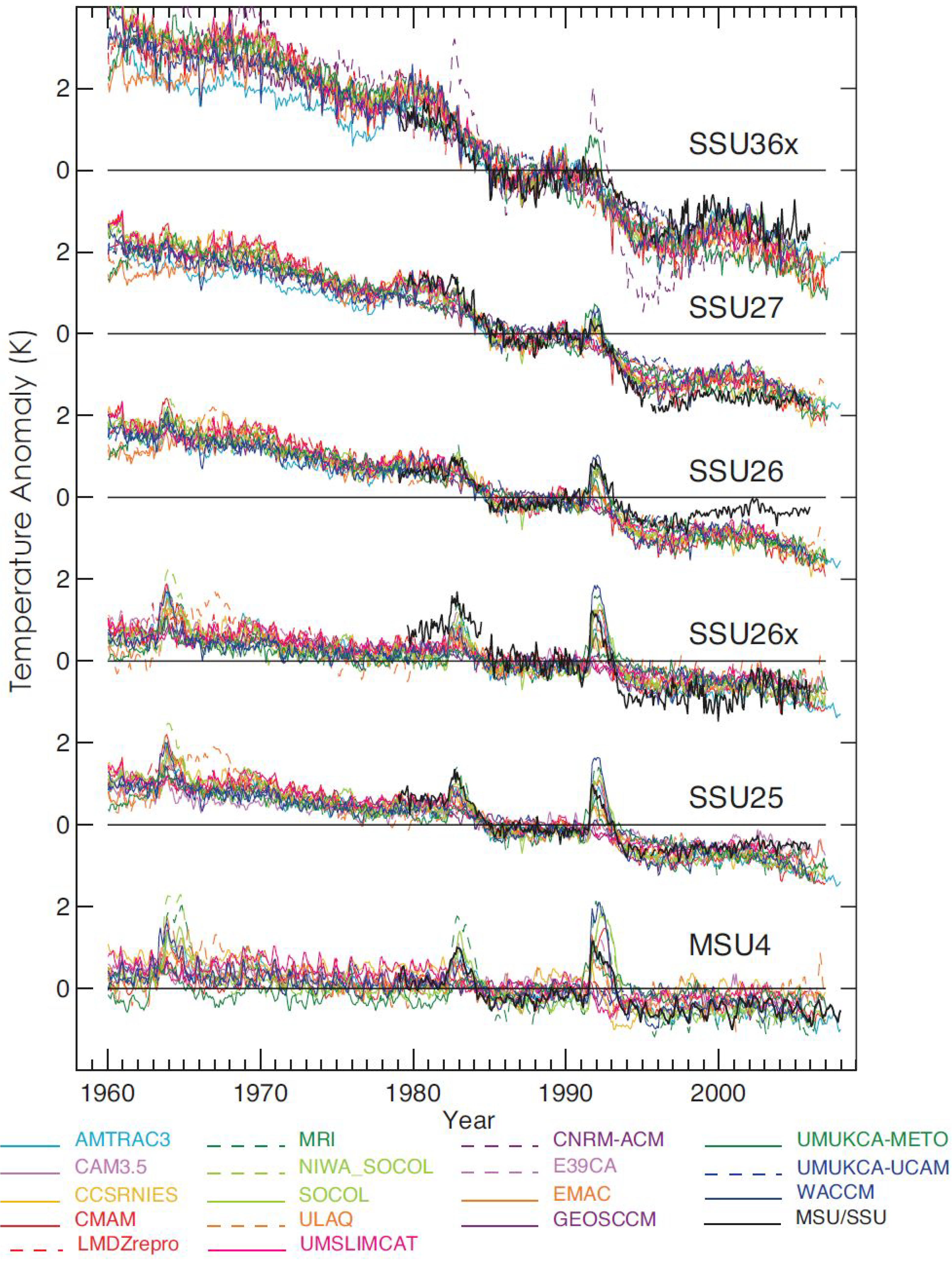
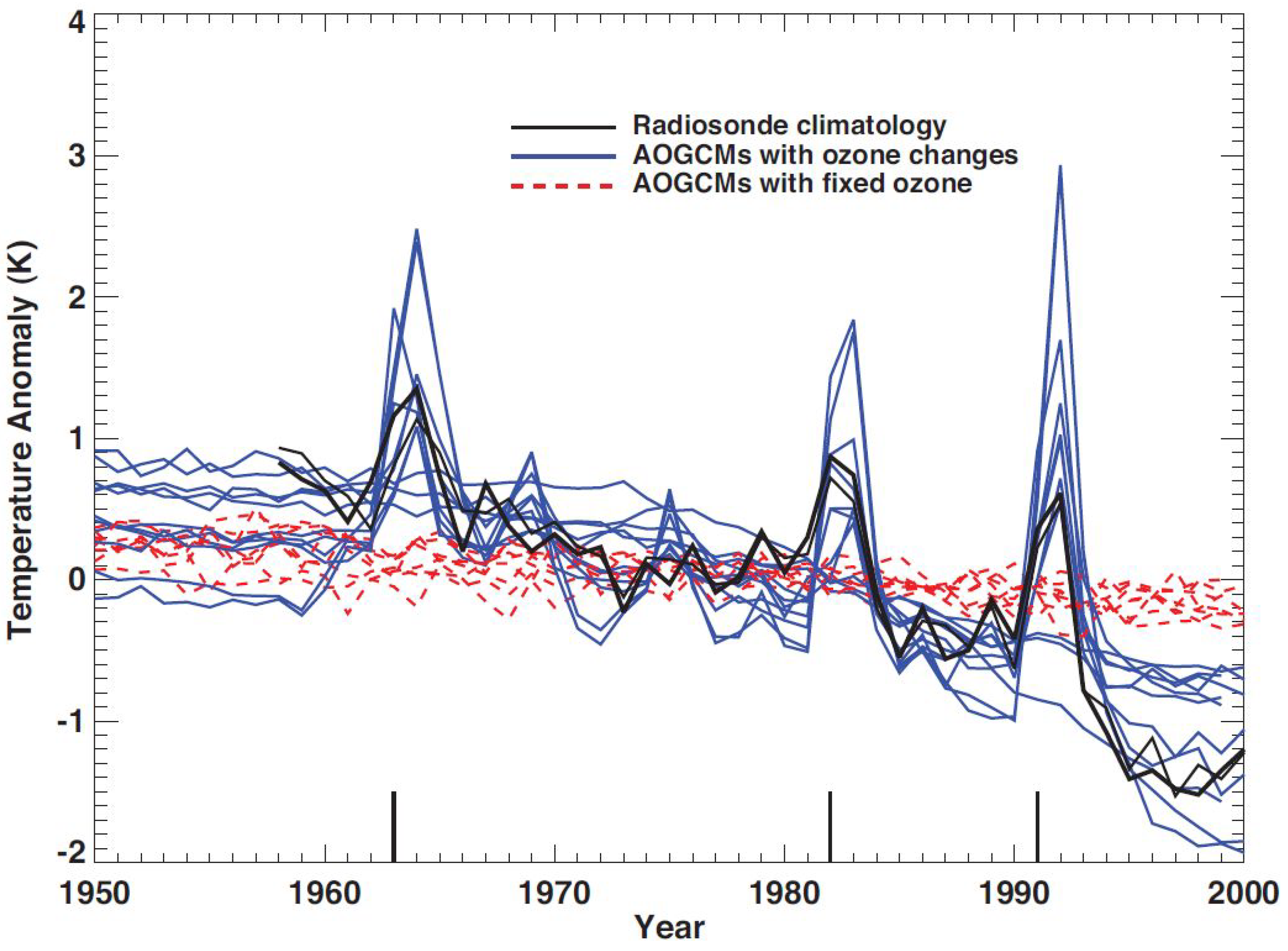
3.2.1. Evolution of Stratospheric Temperature

An example of the complex interplay of dynamics, chemical composition and radiative feedback is the evolution of stratospheric temperatures in recent decades. The thermal structure of the stratosphere is affected by both natural and anthropogenic factors. Several studies have been performed to describe the spatio-temporal structure of stratospheric temperature, in particular the observed cooling [38,39,40]. Attribution of stratospheric temperature variations and long-term changes has been undertaken through comparison of observed changes with simulations by global climate models and CCMs. Ramaswamy et al. [40] showed that the observed cooling of the global lower stratosphere since the late 1970s occurred in two distinct step-like transitions. Subsequent two to three year periods of significant stratospheric warming, due to enhanced sulfate-aerosol loading of the stratosphere following the major volcanic eruptions of El Chichón (in April 1982) and Pinatubo (in June 1991), obvious cooling time periods were followed by a period of relatively steady temperatures. Ramaswamy and colleagues showed that stratospheric cooling was largely attributable to the combined effect of stratospheric ozone depletion and increases of greenhouse gas concentrations (particularly CO2), super-imposed on natural influences induced by the 11-year solar irradiance variation (solar activity cycle) and the intended volcanic eruptions. Simulations performed with CCMs support these findings (Chapter 3 in [3]); most CCMs are able to reproduce adequately the variations and long-term evolution of stratospheric temperature over the last five decades (Figure 2).
Figure 2. Global mean time series of satellite observed (black lines; from [41]) and CCM (colored lines) temperature anomalies (in K) weighted for Microwave Sounding Unit/Stratospheric Sounding Unit (MSU/SSU) weighting functions. The anomalies are calculated with respect to the period of 1980–1994. Exact weighting functions for the MSU/SSU satellite instruments are given in [41]. Channel 27 corresponds to ~34–52 km altitude, channel 36x to ~38–52 km, channel 26 to ~26–46 km, channel 25 to ~20–38 km, channel 26x to ~21–39 km, and channel MSU4 to ~13–22 km. (Figure 4–10 in [2].)
Atmosphere 04 00132 g002
Results derived from CMIP3 climate model simulations (Figure 3) in general show less agreement with the radiosonde climatology; but nevertheless it is demonstrated that the observed global mean cooling trend in the lower stratosphere is clearly underestimated by AOGCMs that do not include the decline of stratospheric ozone concentration over the last three decades [42,43]. This strongly indicates the significant role of stratospheric ozone in connection with climate (see Section 3.2.2). Therefore predictions of the future stratospheric temperature will have a significant bias if the global climate model neglects the expected recovery of the ozone layer.
Figure 3. Time series of globally averaged annual temperature anomalies (K) at 50 hPa from radiosonde observations (black line) and AOGCM simulations (colored lines). Global climate model (AOGCM) simulations that included specified stratospheric ozone depletion, as well as increases in greenhouse gases and anthropogenic aerosols, are shown with blue lines, while model simulations that did not include stratospheric ozone depletion are shown with red dashed lines. Some, but not all, the models also include specified stratospheric volcanic aerosol amounts. Short vertical lines on the abscissa denote years of eruptive volcanic eruptions: Agung (1963), El Chichón (1982), and Pinatubo (1991). (Figures 4–15 in [2]; see also [42]).
Atmosphere 04 00132 g003

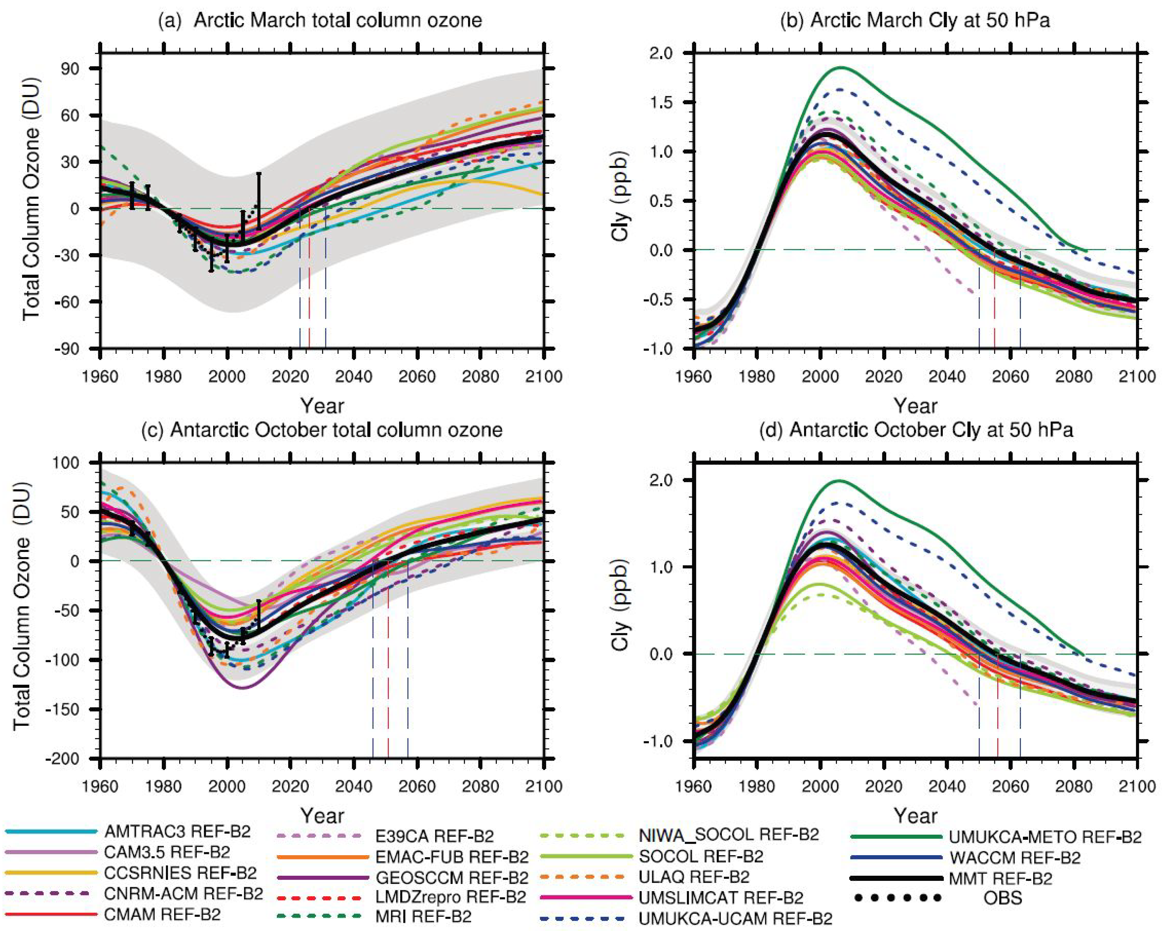
3.2.2. Ozone-Climate Connections

The connection between climate change and the evolution of the stratospheric ozone layer is an outstanding example for climate-chemistry feedback. Changing greenhouse gas concentrations are affecting the thermal structure of the stratosphere (see above). Hence, they should also influence chemical reactions via temperature depending reaction rates (in this case ozone destroying reactions) and modifications of the atmospheric circulation and transport of trace substances. Therefore, it is expected that the return date of the ozone layer to past, undisturbed values not only depends on the decreasing amount of ozone depleting substances (e.g., chlorine), but also on changes of the thermal structure of the atmosphere. A regionally different regeneration of the ozone layer is most likely and will probably not represent a simple reversal of the depletion observed over recent years. For instance, climate change could cause enhanced ozone concentrations particularly in the middle and upper stratosphere compared to undisturbed ozone values (see below) or may prevent the return to prior ozone levels in the tropics ( Chapter 9 in [3]). The situation in polar regions is complex as well.
Figure 4 shows the temporal evolution of total column ozone and corresponding lower stratospheric inorganic chlorine (Cly) as calculated by 17 individual CCMs for March in the Arctic and October in the Antarctic. In addition, a multi-model trend estimate is depicted. The long-term evolution of total column ozone is qualitatively the same as in other regions, like in middle latitudes or in the tropics (not shown). There are obvious quantitative differences among the CCMs (for a detailed discussion see [44]; Chapter 9 in [3]). In the Antarctic, the strongest ozone depletion in the October mean multi-model trend is simulated in 2003. The minimum total column ozone is about 80 DU lower than the 1980 value. In the Arctic, the largest total column ozone depletion in March 2002 is only approximately 30% (about 25 DU) of the strongest Antarctic depletion. Arctic spring ozone returns earlier to 1980 values than Antarctic spring ozone: In the Arctic region total ozone is projected to return to 1980 values by about 2025 whereas in Antarctica a full recovery is expected by 2050. Interestingly, the multi model mean for Arctic column ozone in spring is simulated to increase to nearly 50 DU (35 DU) above 1980 (1960) values by the end of the 21st century (“super-recovery” of ozone); in Antarctic spring total ozone is projected to be about 40 DU above 1980 levels. However, by 2100, Antarctic October mean ozone column is still projected to be about 10 DU lower than in 1960.
The reasons for this different regional recovery of stratospheric ozone in the CCMs are due to the continued increase in greenhouse gas concentrations in the atmosphere, particularly CO2. It is expected that the stratosphere will cool down further, resulting in faster ozone-layer regeneration especially in the extra-polar middle and upper stratosphere. There, lower temperatures slow down ozone destroying (temperature depending) chemical reactions. In the lower polar stratosphere, in particular in the Southern Hemisphere, the rebuilding of the ozone layer can be slowed down during spring. There, lower temperatures lead to an increased formation of polar stratospheric clouds (PSCs) which are the necessary prerequisite for ozone depletion [45]. On the other hand, climate change will affect ozone transport from lower to higher latitudes due to the Brewer-Dobson circulation. CCMs predict enhanced transport of ozone rich stratospheric air masses from tropical to extra-tropical regions ([12], Chapter 4 in [3]). The isolation of the Southern Hemisphere polar stratosphere in winter, which is originated by the polar night jet, could prevent an accelerated closure of the Antarctic ozone hole in the models. A quicker re-formation of the ozone layer in the Arctic stratosphere is simulated because on average the polar vortex is less stable due to enhanced planetary wave activity. On the other hand the interhemispheric differences in the recovery of polar ozone may be affected by a poor representation of polar ozone loss due to temperature biases (Chapter 6 in [3]). Another source of uncertainty is the missing consideration of circulation changes on the lifetimes of ozone depleting substances in the models. Overall, CCM simulations indicate that the ozone layer is expected to recover faster in the Arctic than in the Antarctic stratosphere [46]. The predicted super-recovery of the ozone layer seems to be a consequence of climate change in the post-CFC area. For the second half of this century, the majority of CCMs are indicating an ozone layer with larger column ozone values than before the year 1980. The robustness of such a scenario needs to be investigated more strongly as well as the possible consequences for fauna and flora.
Figure 4. 1980 baseline-adjusted multi-CCM trend estimates of annually averaged total column ozone (DU; left) and Cly at 50 hPa (ppb; right) for Arctic (60°–90°N, upper row) and Antarctic (60°–90°S, lower row) (thick dark gray line) with 95% confidence and 95% prediction intervals appearing as light- and dark-gray shaded regions, respectively, about the trend (note the different vertical scale among the panels). Colored lines: The baseline-adjusted individual model trends; red vertical dashed line: year when the multi-model trend in total column ozone (left) and Cly at 50 hPa (right) returns to 1980 values; blue vertical dashed lines: uncertainty in these return dates; black dotted lines in the left panels: observed total column ozone, where a linear least square regression model was used to remove the effects of the quasi-biennial oscillation, solar cycle, El Niño-Southern Oscillation, and volcanoes from four observational data sets. The observations include ground-based measurements (updated from [47]), merged satellite data [48], the National Institute of Water and Atmospheric Research (NIWA) combined total column ozone database [49], and Solar Backscatter Ultraviolet (SBUV, SBUV/2) retrievals (updated from [50]). The observational time series is shifted vertically so that it equals 0 in 1980. (Figures 3–11 in [2].)
Atmosphere 04 00132 g004

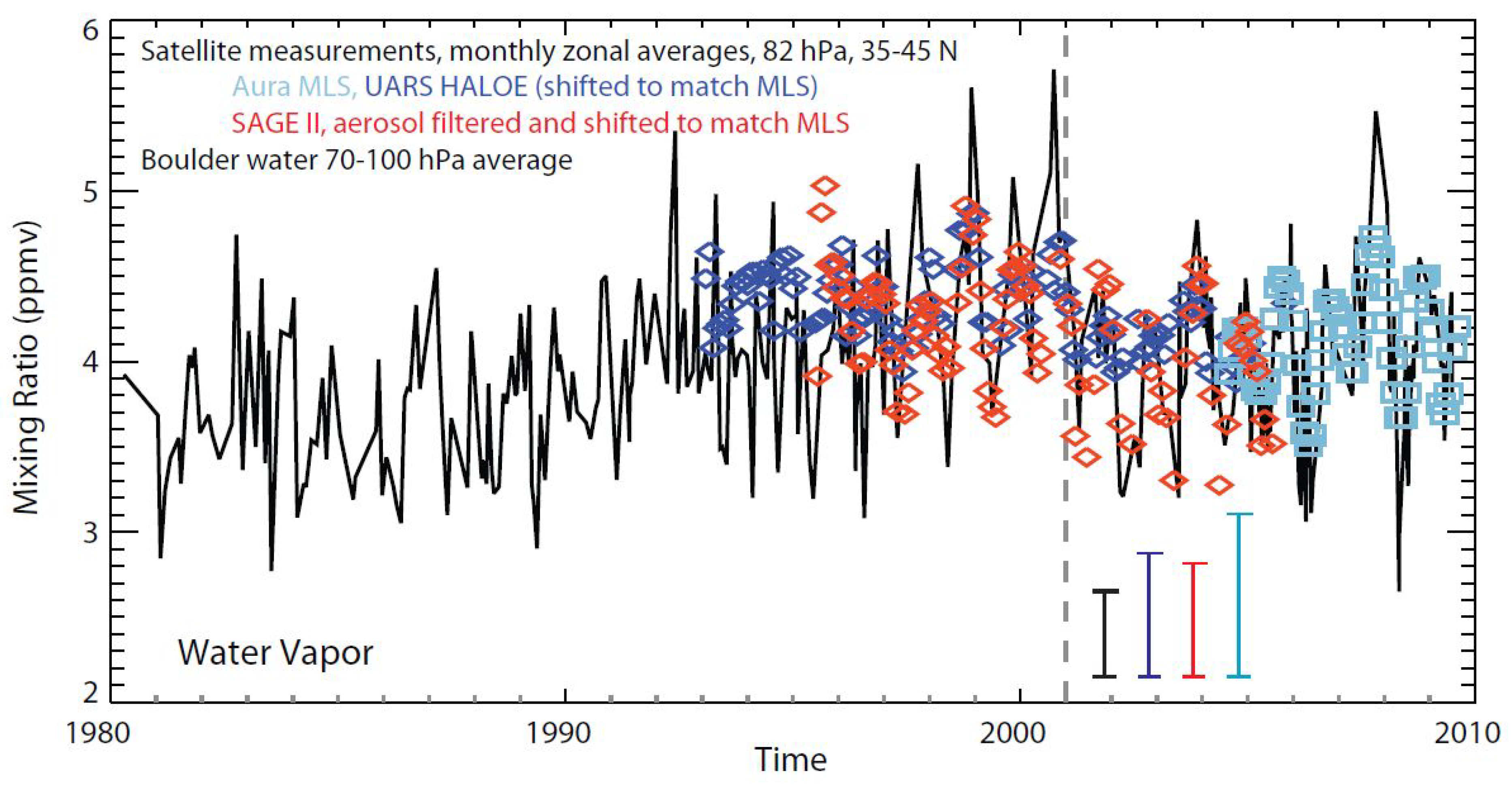
3.2.3. Water Vapor in the Stratosphere

Water vapor is the most relevant greenhouse gas. Therefore, it is extremely important to understand fluctuations of water vapor concentrations in the troposphere and stratosphere as well as their trends. Most CCMs are able to reproduce the annual cycle of water vapor in the tropical lower stratosphere (i.e., the region where water vapor enters the stratosphere) with a minimum in Northern Hemisphere spring and a maximum in Northern Hemisphere fall and winter. Nevertheless, absolute values derived from different CCM simulations show a large spread (Figures 4–13 in [2]). To verify long-term changes in the lower stratospheric water vapor concentration, the only consistent multi-decadal time series of stratospheric water vapor content is limited to Northern Hemisphere middle latitudes, derived from frost point balloon measurements taken from Boulder, Colorado (40°N) [51]. First observations from satellite instruments were performed in 1992 [52]. Until today several instruments have continued water vapor measurements from space. Using overlap periods between instruments, it is possible to determine consistent long-term time series allowing the detection of global trends. The complete water vapor data set of actual Boulder is shown in Figure 5 together with time series from satellite instruments HALOE, SAGE II, and Aura MLS [53].
Figure 5. Observed changes in stratospheric water vapor. Time series of stratospheric water vapor mixing ratio (ppmv) averaged from 70 to 100 hPa near Boulder Colorado (40°N, 105.25°W) from a balloon-borne frost point hygrometer covering the period 1981 through 2009; satellite measurements are monthly averages, balloon data plotted are from individual flights. Also plotted are zonally averaged satellite measurements in the 35°N–45°N latitude range at 82 hPa from the Aura MLS (turquoise squares), UARS HALOE (blue diamonds), and SAGE II instruments (red diamonds). (Figure 4-2 in Chapter 4 of [2]; see also [53].)
Atmosphere 04 00132 g005
Analyses have indicated that changes in methane mixing ratio only explain parts of the trend. So far, the reason for the residuary increase of water vapor mixing ratio for the period ending in 2000 is still unclear [54,55,56,57]. Since the end of 2000, an obvious reduction in the amount of water vapor entering the tropical stratosphere occurred [58,59], which was accompanied by a drop in tropical tropopause temperatures that occurred during a period without an increase of methane concentration [60]. The drop in tropical tropopause temperature and reduced entry of water vapor into the stratosphere at the end of 2000 appears to be connected to an enhanced rate of tropical upwelling [58,59] and associated changes in eddy wave driving [61]. Moreover, there is still no agreement about the cause-effect-chain for the strengthening of tropical upwelling near the tropical tropopause; both tropical SST changes [62] and changes in high-latitude wave forcing [63] have been suggested. Another hint for an insufficient understanding of atmospheric processes determining the variability of tropopause temperature and not least the water vapor content in the lower stratosphere is that by now, no CCM has simulated a similar sharp decrease of tropopause temperature or water vapor concentration at any specific period during multi-decadal simulations. Therefore, future predictions of stratospheric water vapor, and how it may influence climate change, are highly uncertain. This is an example for an important climate research issue, especially of chemistry-climate change feedbacks, indicating the incomplete understanding of the complex climate system. Further investigation on the basis of observations and numerical model studies are required.

4. Future Developments and Challenges

4.1. From Chemistry-Climate Models to Earth-System Models

More detailed analyses of the complex connections between the atmospheric sub-systems (dynamics and chemistry) and the boundary conditions (SSTs, SIC, land and ocean biosphere dynamics, solar variability, chemical interactions between atmosphere and ocean and biosphere, etc.) require increasingly complex model systems. This constitutes a fundamental dilemma of computational Earth-System Sciences: The real system in its full complexity is far from being entirely understood and the tools to improve our understanding (the models) need themselves to become more and more complex. This development bears on the one hand side the risk of misinterpreting the simulation results, because results become increasingly difficult to understand, and on the other hand lacks a clear strategy on how exactly the models should be expanded. So far the only reasonable strategy is to combine existing approaches of different domains (atmosphere, ocean, sea ice, land-surface biosphere, soil, etc.) into comprehensive ESMs. In order to prevent that simulation results with “all-encompassing” model systems become unwieldy for some problems that do not need all the details, modular approaches with individually suitable sub-components are highly feasible. Sensitivity studies with comprehensive model systems operated in different but internally consistent modes of complexity provide useful information. Beside extensive model approaches in future there will be a necessity for simplified models with reduced complexity to study sub-systems or certain classes of problems.
Since simulation results become increasingly difficult to understand, additional efforts of implementing advanced on-line diagnostic techniques are required; for instance, to simplify the inter-comparison with observations [64,65,66] or to quantify the contribution of different processes to the simulations results [67].
Another limitation of the state-of-the art global climate and climate-chemistry model systems is their truncated range of resolved spatial scales. This limitation has required sub-grid-scale parameterizations of important processes (e.g., clouds, convection, tropical cyclone activity, gravity waves, etc.). This, on the one hand side introduces considerable uncertainties and on the other hand side renders understanding the role of regional processes difficult. Investigating the role of global changes for regional processes and climate is usually based on statistical or dynamical downscaling methods. The latter, for instance, involves nesting of a finer resolved limited area model (LAM) off-line into a global model, meaning that the lateral boundary conditions for the LAM are taken from global AGCM, AOGCM or CCM output. These approaches do, however, not allow any feedback from the smaller (LAM) scales back to the global scale. To overcome this limitation, new developments aim at global cloud resolving models [68]. This approach is, however, due to computational constraints (see next section) at the time being only feasible for NWP models and probably AGCMs. For CCMs, which require enormous amounts of computational resources for simulating the chemistry subsystem, a promising approach is the two-way nesting of a chemistry enabled LAM into a global CCM at the region of interest (for first steps into this direction, i.e., a one-way on-line nesting approach, see [69]). With such an approach, climate relevant hot-spots can then be simulated at higher resolution than the rest of the domain. A proof of concept for this approach is still pending. Due to increasing computer power the ability to run global models at ever-higher horizontal resolutions (i.e., less than about 100 km) becomes possible, but this requires a systematic investigation of the impact of spatial resolution on simulation results independent of the model formulation [70].

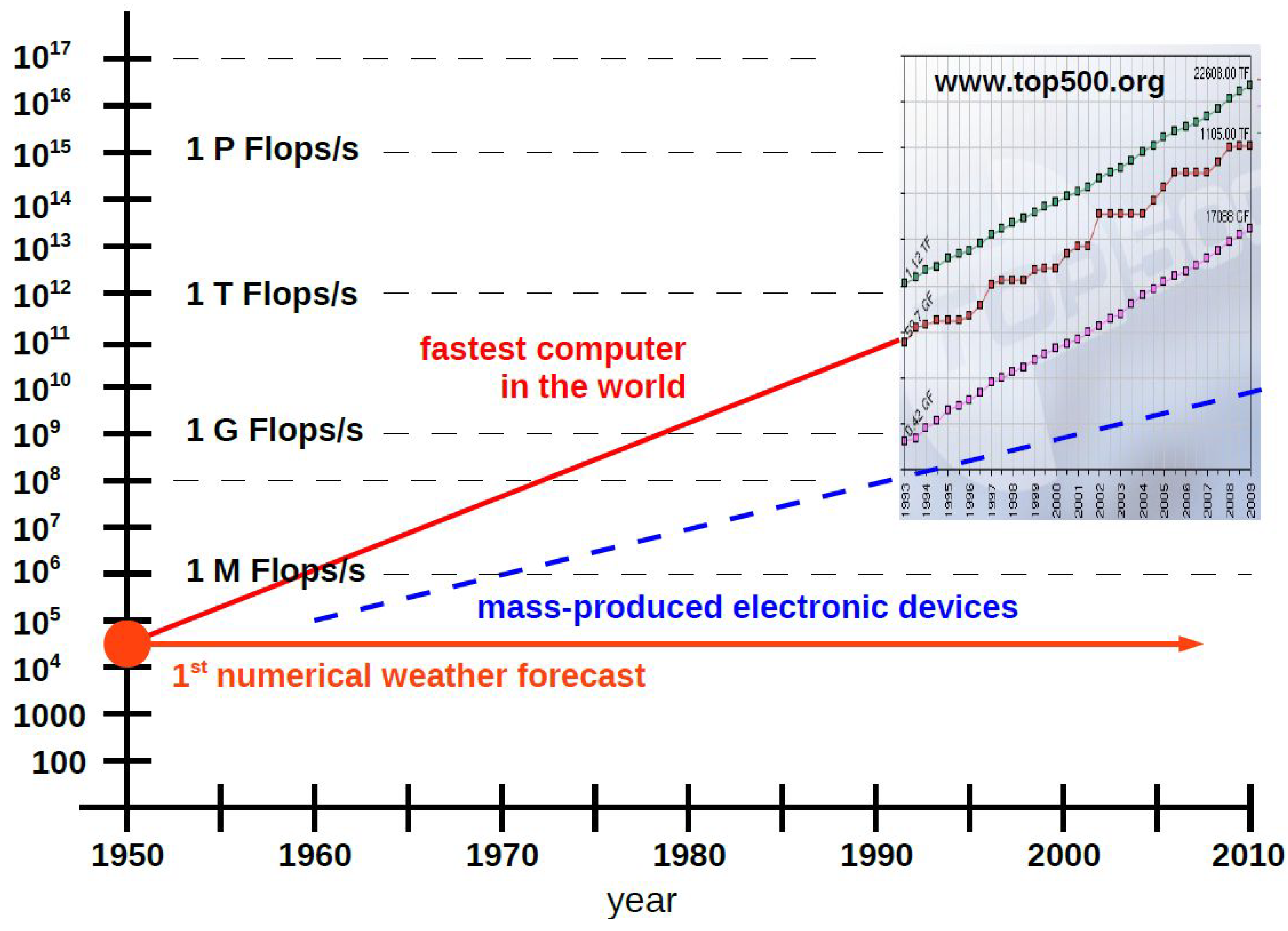
4.2. Use of the Next Computer Generation: Challenges for Atmospheric Science

The technical challenges for computational Earth-System Sciences (including atmospheric research) are manifold. First, as mentioned above, the model systems become increasingly complex by taking into account more and more processes and feedbacks. Second, the resolution becomes finer in order to resolve more processes reducing the necessity to parameterize them as sub-grid-scale processes. In order to keep these model systems controllable and understandable, the application of software engineering methodologies for development and maintenance of the underlying codes is clearly required. This need is augmented by the fact that the model software life cycles are usually much longer (decades) than the life cycles of the high-end super-computer systems they are running on (5–10 years). In the context of developing and maintaining such complex model systems, another open question is about the best suited strategy on how to technically couple the different components or domains (see section above) together into a single comprehensive model. An overview of different methods can be found in ([69], Appendix A). Finally, increasing complexity and resolution imply a likewise increasing amount of model output data, which needs to be stored, post-processed and further analyzed. The application of new, fast data mining techniques and statistical analyses needs to be complemented by newly developed on-line model diagnostics and for data reduction (see also section above). In the future, it might become increasingly appropriate to redo a complete model simulation with additional on-line diagnostics or alternative model output (tailor made to answer a specific scientific question) instead of the current approach of storing the entire (or at least a large part of) model output for later analysis. This holds in particular for non-hydrostatic models which can be operated at very high resolution.
Complementary to the increasing complexity and resolution of computational models, the computer systems are about to change with considerable impact for the scientific model development. Moore’s Law [71], in essence predicting the doubling of possible computational power in terms of achievable floating point operations per second (FLOPS/s) every 18–24 months, was in the past sustained by the increase of integrated circuits per chip area and by a steadily increasing clock rate of the transistors (Figure 6).
Figure 6. Performance of computational devices (in floating point operations (Flops) per second) over time from [72] (upper right inlay) extrapolated back to 1950 when the first numerical weather forecast (24 h forecast time, 24 h computation) has been performed [73]. The similar increase in computational performance of mass-produced electronic devices (dashed blue line) enabled Lynch and Lynch [74] to repeat this 1st 24 h weather forecast (as Java application) on a customary cell phone in less than 1 s.
Atmosphere 04 00132 g006
This development implied that every new chip generation guaranteed an increase in model run time performance at almost no additional cost concerning the software development, meaning the code executed faster on newer processors with almost no modifications. This period of increasing single chip performance, however, has come to an end, mainly because transistor density cannot be increased ad infinitum and because power consumption increases over-proportionally with clock rate and thus the energy costs start to exceed economically justifiable limits. Sustaining Moore’s Law in the future therefore requires completely new technologies that are not yet available, at least not beyond the laboratory state. The current developments therefore focus on an increased parallelism, essentially implying the application of a much larger number of computational units, each with a largely reduced computational power (and memory) and therefore with a reduced integrated power consumption. Common to all developing technologies, multi-core/many-core systems, hybrid systems with accelerators such as graphical processing units (GPUs), etc. is the need for highly parallelized applications, shall the resources be efficiently used and the performance be increased. This parallelism requires completely new algorithmic and numerical approaches. Given the complexity of the models, which usually combine several numerical schemes for different processes (e.g., to solve ordinary differential equation (ODE) and partial differential equation (PDE) systems) in an operator splitting approach, the task to adapt state-of-the-art model systems to the new computer architectures is not trivial and requires specialized skills in programming techniques and software engineering. With the newly emerging architectures it might be necessary to replace even well-established programming models and known parallelization techniques (such as OpenMP for shared and MPI for distributed memory parallelization), for instance making use of newly developing programming models, such as “Partitioned Global Address Space” (PGAS).

5. Concluding Remarks

Today, numerical modeling is an important part of atmospheric and climate research. Results of model simulations serve to investigate the role of individual atmospheric processes and their interaction (e.g., feedback of dynamics and chemistry), as well as the coupling of different atmospheric layers, for instance the stratosphere and the troposphere, or linking of the atmosphere with oceans. The use of models on the one hand helps in the study and understanding of complex connections in the Earth climate system; on the other hand it discloses gaps in our understanding of atmospheric behavior. The detailed evaluation of results derived from numerical model simulations with observations (but also with results from other models) is necessary to identify strengths and weaknesses of the applied models. In particular, detection of discrepancies between the “real” and the “model” world is pointing to missing processes in the model systems or at least inaccuracies in the description of atmospheric processes and interactions. The overall aim is to develop models representing atmospheric conditions as best as possible (e.g., good representation of climatological mean conditions, variability on shorter and longer time-scales, trends), providing the best possible basis for future projections according to assumed scenarios. Evaluated models systems are essential requirements for assessments of the future evolution of atmospheric conditions and climate change. Outstanding successful examples for this kind of research are the CMIP3/CMIP5 activities for the recent 4th Assessment Report of IPCC [1] and the scheduled 5th Assessment Report (will be published in 2013/2014) and the SPARC CCMVal activity in connection with the WMO ozone reports [2,20].
Currently there are many efforts world-wide to build up more comprehensive model systems, so-called Earth-System Models (ESMs), considering as many as possible components describing the Earth climate system, for instance, the carbon cycle, the biosphere, the cryosphere, or land surfaces. It is not only a challenging task to couple correctly the individual models describing sub-systems, but also to interpret the results of such complex systems. The more individual processes and feedback effects are considered in coupled model systems like ESMs, the more difficult is the assignment of cause-effects-chains explaining particular results. Therefore it is important to further develop massive on-line diagnostics and use in parallel simplified models for basic research, not only the “atmosphere only” models like the AGCMs and CCMs, but also even simpler models, e.g., mechanistic models or process models. This allows additive fundamental, more process-oriented investigations, which are in principle easier to interpret and require less computer resources.
Another great challenge in future is the adaptation of the currently used model systems to the next generation of super-computers. This is not straightforward and involves particular skills not only in programming techniques but also software engineering. In some cases the numerical codes have to be completely changed, in other cases, at least, they must be significantly revised. Most of the currently used atmospheric models have been developed over years and so far are not ready for optimal usage of computer systems available in future.
We are proceeding from the assumption that in the next years the application of numerical modeling will become more diverse in atmosphere and climate research areas. But differently to recent years, further developments are necessary not only from the viewpoint of climate (or Earth-system) science, but also especially with regard to an adequate use of the quickly developing super-computers. Here a more intensive collaboration of subject-specific scientists is highly required, both from the specialist discipline and applied computer science.

Acknowledgements

We are grateful to Volker Grewe and Rudolf Deckert for helpful comments on the manuscript.

Conflict of Interest

The authors declare no conflict of interest.

References

  1. Intergovernmental Panel on Climate Change (IPCC), Climate Change 2007: The Physical Science Basis—Contribution of Working Group I to the Fourth Assessment Report of the Intergovernmental Panel on Climate Change; Solomon, S.; Qin, D.; Manning, M.; Chen, Z.; Marquis, M.; Averyt, K.B.; Tignor, M.; Miller, H.L. (Eds.) Cambridge University Press: Cambridge, UK/New York, NY, USA, 2007; p. 996.
  2. World Meteorological Organization (WMO)/United Nations Environment Programme (UNEP), Scientific Assessment of Ozone Depletion: 2010; Global Ozone Research and Monitoring Project-Report No. 52; WMO/UNEP: Geneva, Switzerland, 2011; p. 516.
  3. Eyring, V.; Shepherd, T.G.; Waugh, D.W. (Eds.) Stratospheric Processes and Their Role in Climate (SPARC) Chemistry-Climate Model Validation Activity (CCMVal). SPARC Report on the Evaluation of Chemistry-Climate Models. 2010. Available online: http://www.atmosp.physics.utoronto.ca/SPARC (accessed on 1 June 2010).
  4. Crutzen, P. Albedo enhancement by stratospheric sulfur Injections: A contribution to resolve a policy dilemma? Clim. Change 2006, 77, 211–220. [Google Scholar] [CrossRef]
  5. Heckendorn, P.; Weisenstein, D.; Fueglistaler, S.; Luo, B.P.; Rozanov, E.; Schraner, M.; Thomason, L.W.; Peter, T. Impact of geoengineering aerosols on stratospheric temperature and ozone. Environ. Res. Lett. 2009, 4, 045108. [Google Scholar] [CrossRef]
  6. Pierce, J.R.; Weisenstein, D.K.; Heckendorn, P.; Peter, T.; Keith, D.W. Efficient formation of stratospheric aerosol for climate engineering by emission of condensable vapor from aircraft. Geophys. Res. Lett. 2010. [Google Scholar] [CrossRef]
  7. Jeuken, A.B.M.; Siegmund, P.C.; Heijboer, L.C.; Feichter, J.; Bengtsson, L. On the potential of assimilating meteorological analyses in a global climate model for the purpose of model validation. J. Geophys. Res. 1996, 101, 16939–16950. [Google Scholar]
  8. Jöckel, P.; Tost, H.; Pozzer, A.; Brühl, C.; Buchholz, J.; Ganzeveld, L.; Hoor, P.; Kerkweg, A.; Lawrence, M.G.; Sander, R.; et al. The atmospheric chemistry general circulation model ECHAM5/MESSy1:Consistentsimulation of ozone from the surface to the mesosphere. Atmos. Chem. Phys. 2006, 6, 5067–5104. [Google Scholar] [CrossRef]
  9. Thomas, G.; Marsh, D.; Lübken, F.-J. Mesospheric ice clouds as indicators of upper atmosphere climate change: Workshop on modeling polar mesospheric cloud trends; Boulder, Colorado, 10–11 December 2009. EOS Trans. AGU 2010, 91, 183. [Google Scholar] [CrossRef]
  10. Berger, U.; Lübken, F.-J. Mesospheric temperature trends at mid-latitudes in summer. Geophys. Res. Lett. 2011, 38, L22804. [Google Scholar]
  11. Lübken, F.-J.; Berger, U.; Kiliani, J.; Baumgarten, G.; Fiedler, J. Solar Variability and Trend Effects in Mesospheric Ice Layers. In Climate and Weather of the Sun-Earth System (CAWSES): Highlights from a Priority Program; Springer: Dordrecht, The Netherlands, 2012. [Google Scholar]
  12. Butchart, N.; Scaife, A.A.; Bourqui, M.; de Grandpré, J.; Hare, S.H.E.; Kettleborough, J.; Langematz, U.; Manzini, E.; Sassi, F.; Shibata, K.; et al. Simulations of anthropogenic change in the strength of the Brewer–Dobson circulation. Clim. Dyn. 2006, 27, 727–741. [Google Scholar] [CrossRef]
  13. Garny, H.; Dameris, M.; Randel, W.; Bodeker, G.E.; Deckert, R. Dynamically forced increase of tropical upwelling in the lower stratosphere. J. Atmos. Sci. 2011, 68, 1214–1233. [Google Scholar] [CrossRef]
  14. Shepherd, T.G.; McLandress, C. A robust mechanism for strengthening of the Brewer–Dobson Circulation in response to climate change: Critical-layer control of subtropical wave breaking. J. Atmos. Sci. 2011, 68, 784–797. [Google Scholar] [CrossRef]
  15. Meehl, G.A.; Covey, C.; Delworth, T.; Latif, M.; McAvaney, B.; Mitchell, J.F.B.; Stouffer, R.J.; Taylor, K.E. The WCRP CMIP3 multi-model dataset: A new era in climate change research. Bull. Am. Meteorol. Soc. 2007, 88, 1383–1394. [Google Scholar] [CrossRef]
  16. Knutti, R.; Furrer, R.; Tebaldi, C.; Cermak, J.; Meehl, G.A. Challenges in combining projections from multiple models. J. Clim. 2010, 23, 2739–2756. [Google Scholar] [CrossRef]
  17. Chipperfield, M.P.; Pyle, J.A. Model sensitivity studies of Arctic ozone depletion. J. Geophys. Res. 1998, 103, 389–403. [Google Scholar]
  18. Grewe, V.; Dameris, M.; Hein, R.; Sausen, R.; Steil, B. Future changes of the atmospheric composition and the impact of climate change. Tellus 2001, 53, 103–121. [Google Scholar]
  19. Sinnhuber, B.-M.; Stiller, G.; Ruhnke, R.; von Clarmann, T.; Kellmann, S.; Aschmann, J. Arctic winter 2010/2011 at the brink of an ozone hole. Geophys. Res. Lett. 2011, 38, L24814. [Google Scholar]
  20. World Meteorological Organization (WMO), Scientific Assessment of Ozone Depletion: 2006. Global Ozone Research and Monitoring Project-Report No. 50; WMO: Geneva, Switzerland, 2007; p. 572.
  21. Lelieveld, J.; Brühl, C.; Jöckel, P.; Steil, B.; Crutzen, P.J.; Fischer, H.; Giorgetta, M.A.; Hoor, P.; Lawrence, M.G.; Sausen, R.; Tost, H. Stratospheric dryness: Model simulations and satellite observations. Atmos. Chem. Phys. 2007, 7, 1313–1332. [Google Scholar] [CrossRef]
  22. Schumann, U.; Huntrieser, H. The global lightning-induced nitrogen oxides source. Atmos. Chem. Phys. 2007, 7, 3823–3907. [Google Scholar] [CrossRef]
  23. Kurz, C. Entwicklung und Anwendung eines gekoppelten Klima-Chemie-Modellsystems: Globale Spurengastransporte und chemische Umwandlungsprozesse. Ph.D. Thesis, Institut für Luft- und Raumfahrtmedizin (DLR), Forschungsbericht, Germany, 2007; p. 142. [Google Scholar]
  24. Tost, H.; Lawrence, M.G.; Brühl, C.; Jöckel, P.; The GABRIEL Team; The SCOUT-O3-DARWIN/ACTIVE Team. Uncertainties in atmospheric chemistry modelling due to convection parameterisations and subsequent scavenging. Atmos. Chem. Phys. 2010, 10, 1931–1951. [Google Scholar] [CrossRef]
  25. Grewe, V.; Moussiopoulos, N.; Builtjes, P.; Borrego, C.; Isaksen, I.S.A.; Volz-Thomas, A. The ACCENT-protocol: A framework for benchmarking and model evaluation. Geosci. Model Dev. 2012, 5, 611–618. [Google Scholar] [CrossRef]
  26. WCRP CMIP3 Sub-Project Publications. Available online: http://www-pcmdi.llnl.gov/ipcc/subproject_publications.php (accessed on 9 January 2013).
  27. List of CCMVal Publications. Available online: http://www.pa.op.dlr.de/CCMVal/CCMVal_publications.html (accessed on 11 September 2012).
  28. Telford, P.J.; Braesicke, P.; Morgenstern, O.; Pyle, J.A. Technical note: Description and assessment of a nudged version of the new dynamics unified model. Atmos. Chem. Phys. 2008, 8, 1701–1712. [Google Scholar] [CrossRef]
  29. Liu, C.; Beirle, S.; Butler, T.; Liu, J.; Hoor, P.; Jöckel, P.; Pozzer, A.; Frankenberg, C.; Lawrence, M.G.; Lelieveld, J.; et al. Application of SCIAMACHY and MOPITT CO total column measurements to evaluate model results over biomass burning regions and Eastern China. Atmos. Chem. Phys. 2011, 11, 6083. [Google Scholar] [CrossRef] [Green Version]
  30. Pozzer, A.; Jöckel, P.; Tost, H.; Sander, R.; Ganzeveld, L.; Kerkweg, A.; Lelieveld, J. Simulating organic species with the global atmospheric chemistry general circulation model ECHAM5/MESSy1: A comparison of model results with observations. Atmos. Chem. Phys. 2007, 7, 2527. [Google Scholar] [CrossRef]
  31. Brühl, C.; Steil, B.; Stiller, G.; Funke, B.; Jöckel, P. Nitrogen compounds and ozone in the stratosphere: comparison of MIPAS satellite data with the chemistry climate model ECHAM5/MESSy1. Atmos. Chem. Phys. 2007, 7, 5585. [Google Scholar] [CrossRef]
  32. Baumgaertner, A.J.G.; Jöckel, P.; Riede, H.; Stiller, G.; Funke, B. Energetic particle precipitation in ECHAM5/MESSy Part 2: Solar proton events. Atmos. Chem. Phys. 2010, 10, 7285. [Google Scholar] [CrossRef]
  33. van Aalst, M.K.; van den Broek, M.M.P.; Bregman, A.; Brühl, C.; Steil, B.; Toon, G.C.; Garcelon, S.; Hansford, G.M.; Jones, R.L.; Gardiner, T.D.; et al. Trace gas transport in the 1999/2000 Arctic winter: comparison of nudged GCM runs with observations. Atmos. Chem. Phys. 2004, 4, 81–93. [Google Scholar] [CrossRef]
  34. Wetzel, G.; Oelhaf, H.; Kirner, O.; Friedl-Vallon, F.; Ruhnke, R.; Ebersoldt, A.; Kleinert, A.; Maucher, G.; Nordmeyer, H.; Orphal, J. Diurnal variations of reactive chlorine and nitrogen oxides observed by MIPAS-B inside the January 2010 Arctic vortex. Atmos. Chem. Phys. 2012, 12, 6581. [Google Scholar] [CrossRef]
  35. Klippel, T.; Fischer, H.; Bozem, H.; Lawrence, M.G.; Butler, T.; Jöckel, P.; Tost, H.; Martinez, M.; Harder, H.; Regelin, E.; et al. Distribution of hydrogen peroxide and formaldehyde over Central Europe during the HOOVER project. Atmos. Chem. Phys. 2011, 11, 4391. [Google Scholar] [CrossRef]
  36. Telford, P.J.; Braesicke, P.; Morgenstern, O.; Pyle, J.A. Reassessment of causes of ozone column variability following the eruption of Mount Pinatubo using a nudged CCM. Atmos. Chem. Phys. 2009, 9, 4251–4260. [Google Scholar]
  37. Van Aalst, M.K.; Lelieveld, J.; Steil, B.; Brühl, C.; Jöckel, P.; Giorgetta, M.A.; Roelofs, G.-J. Stratospheric temperatures and tracer transport in a nudged 4-year middle atmosphere GCM simulation. Atmos. Chem. Phys. Discuss. 2005, 5, 961–1006. [Google Scholar] [CrossRef]
  38. Tost, H.; Jöckel, P.; Lelieveld, J. Influence of different convection parameterisations in a GCM. Atmos. Chem. Phys. 2006, 6, 5475. [Google Scholar] [CrossRef]
  39. Tost, H.; Jöckel, P.; Lelieveld, J. Lightning and convection parameterisations—Uncertainties in global modeling. Atmos. Chem. Phys. 2007, 7, 4553. [Google Scholar] [CrossRef]
  40. Ramaswamy, V.; Schwarzkopf, M.D.; Randel, W.J.; Santer, B.D.; Soden, B.J.; Stenchikov, G.L. Anthropogenic and natural influences in the evolution of lower stratospheric cooling. Science 2006, 311, 1138–1141. [Google Scholar] [CrossRef]
  41. Randel, W.J.; Shine, K.P.; Austin, J.; Barnett, J.; Claud, C.; Gillett, N.P.; Keckhut, P.; Langematz, U.; Lin, R.; Long, C.; et al. An update of observed stratospheric temperature trends. J. Geophys. Res. 2009, 114, D02107. [Google Scholar] [CrossRef]
  42. Cordero, E.C.; Forster, P.M.de F. Stratospheric variability and trends in models used for the IPCC AR4. Atmos. Chem. Phys. 2006, 6, 5369–5380. [Google Scholar] [CrossRef]
  43. Son, S.-W.; Gerber, E.P.; Perlwitz, J.; Polvani, L.M.; Gillett, N.P.; Seo, K.-H.; Eyring, V.; Shepherd, T.G.; Waugh, D.; Akiyoshi, H.; et al. Impact of stratospheric ozone on Southern Hemisphere circulation change: A multimodel assessment. J. Geophys. Res. 2010, 115, D00M07. [Google Scholar] [CrossRef]
  44. Austin, J.; Scinocca, J.; Plummer, D.; Oman, L.; Waugh, D.; Akiyoshi, H.; Bekki, S.; Braesicke, P.; Butchart, N.; Chipperfield, M.; et al. Decline and recovery of total column ozone using a multimodel time series analysis. J. Geophys. Res. 2010, 115, D00M10. [Google Scholar] [CrossRef]
  45. Dameris, M. Climate change and atmospheric chemistry: How will the stratospheric ozone layer develop? Angew. Chem. Int. 2010, 49, 8092–8102. [Google Scholar] [CrossRef] [Green Version]
  46. Dameris, M.; Loyola, D. Chapter 1. Chemistry-Climate Connections—Interaction of Physical, Dynamical, and Chemical Processes in Earth Atmosphere. In Climate Change—Geophysical Foundations and Ecological Effects; Blanco, J., Kheradmand, H., Eds.; InTech: Rijeka, Croatia, 2011; pp. 3–24. [Google Scholar]
  47. Fioletov, V.E.; Bodeker, G.E.; Miller, A.J.; McPeters, R.D.; Stolarski, R. Global and zonal total ozone variations estimated from ground based and satellite measurements: 1964–2000. J. Geophys. Res. 2002, 107, 4647. [Google Scholar]
  48. Stolarski, R.S.; Frith, S.M. Search for evidence of trend slow-down in the long-term TOMS/SBUV total ozone data record: The importance of instrument drift uncertainty. Atmos. Chem. Phys. 2006, 6, 4057–4065. [Google Scholar] [CrossRef]
  49. Bodeker, G.E.; Shiona, H.; Eskes, H. Indicators of Antarctic ozone depletion. Atmos. Chem. Phys. 2005, 5, 2603–2615. [Google Scholar] [CrossRef]
  50. Miller, A.J.; Nagatani, R.M.; Flynn, L.E.; Kondragunta, S.; Beach, E.; Stolarski, R.; McPeters, R.D.; Bhartia, P.K.; DeLand, M.T.; Jackman, C.H.; et al. A cohesive total ozone data set from SBUV(/2) satellite system. J. Geophys. Res. 2002, 107, 4701. [Google Scholar] [CrossRef]
  51. Hurst, D.F.; Oltmans, S.J.; Vömel, H.; Rosenlof, K.H.; Davis, S.M.; Ray, E.A.; Hall, E.G.; Jordan, A.F. Stratospheric water vapor trends over Boulder, Colorado: Analysis of the 30 year Boulder record. J. Geophys. Res. 2011, 116, D02306. [Google Scholar] [CrossRef]
  52. Nedoluha, G.; Gomez, R.M.; Hicks, B.C.; Bevilacqua, R.M.; Russell, J.M.; Connor, B.J.; Lambert, A. A comparison of middle atmospheric water vapor as measured by WVMS, EOS-MLS, and HALOE. J. Geophys. Res. 2007, 112, D24S39. [Google Scholar]
  53. Solomon, K.; Rosenlof, H.; Portmann, R.W.; Daniel, J.S.; Davis, S.M.; Sanford, T.J.; Plattner, G.-K. Contributions of stratospheric water vapor to decadal changes in the rate of global warming. Science 2010, 327, 1219–1223. [Google Scholar]
  54. Zhou, X.-L.; Geller, M.A.; Zhang, M. Cooling trend of the tropical cold point tropopause temperatures and its implications. J. Geophys. Res. 2001, 106, 1511–1522. [Google Scholar] [CrossRef]
  55. Rosenlof, K.H. Transport changes inferred from HALOE water and methane measurements. J. Meteorol. Soc. Japan 2002, 80, 831–848. [Google Scholar] [CrossRef]
  56. Sherwood, S. A microphysical connection among biomass burning, cumulus clouds, and stratospheric moisture. Science 2002, 295, 1272–1275. [Google Scholar] [CrossRef]
  57. Notholt, J.; Luo, B.P.; Füeglistaler, S.; Weisenstein, D.; Rex, M.; Lawrence, M.G.; Bingemer, H.; Wohltmann, I.; Corti, T.; Warneke, T.; von Kuhlmann, R.; Peter, T. Influence of tropospheric SO2 emissions on particle formation and the stratospheric humidity. Geophys. Res. Lett. 2005, 32, L07810. [Google Scholar] [CrossRef]
  58. Randel, W.J.; Wu, F.; Vömel, H.; Nedoluha, G.E.; Forster, P. Decreases in stratospheric water vapor after 2001: Links to changes in the tropical tropopause and the Brewer-Dobson circulation. J. Geophys. Res. 2006, 111, D12312. [Google Scholar] [CrossRef]
  59. Rosenlof, K.H.; Reid, G.C. Trends in the temperature and water vapor content of the tropical lower stratosphere: Sea surface connection. J. Geophys. Res. 2008, 113, D06107. [Google Scholar] [CrossRef]
  60. Dlugokencky, E.J.; Bruhwiler, L.; White, J.W.C.; Emmons, L.K.; Novelli, P.C.; Montzka, S.A.; Masarie, K.A.; Lang, P.M.; Crotwell, A.M.; Miller, J.B.; et al. Observational constraints on recent increases in the atmospheric CH4 burden. Geophys. Res. Lett. 2009, 36, L18803. [Google Scholar] [CrossRef]
  61. Dhomse, S.; Weber, M.; Burrows, J. The relationship between tropospheric wave forcing and tropical lower stratospheric water vapor. Atmos. Chem. Phys. 2008, 8, 471–480. [Google Scholar] [CrossRef]
  62. Deckert, R.; Dameris, M. Higher tropical SSTs strengthen the tropical upwelling via deep convection, Geophys. Res. Lett. 2008, 35, L10813. [Google Scholar] [CrossRef]
  63. Ueyama, R.; Wallace, J.M. To what extent does high-latitude wave forcing drive tropical upwelling in the Brewer-Dobson Circulation? J. Atmos. Sci. 2010, 67, 1232–1246. [Google Scholar] [CrossRef]
  64. Klein, S.A.; Jakob, C. Validation and sensitivities of frontal clouds simulated by the ECMWF model. Mon. Wea. Rev. 1999, 127, 2514–2531. [Google Scholar] [CrossRef]
  65. Webb, M.; Senior, C.; Bony, S.; Morcrette, J.J. Combining ERBE and ISCCP data to assess clouds in the Hadley Centre, ECMWF and LMD atmospheric climate models. Clim. Dyn. 2001, 17, 905–922. [Google Scholar] [CrossRef]
  66. Jöckel, P.; Kerkweg, A.; Pozzer, A.; Sander, R.; Tost, H.; Riede, H.; Baumgaertner, A.; Gromov, S.; Kern, B. Development cycle 2 of the Modular Earth Submodel System (MESSy2). Geosci. Model Dev. 2010, 3, 717. [Google Scholar] [CrossRef] [Green Version]
  67. Grewe, V. A generalized tagging method. Geosci. Model Dev. 2013, 6, 247–253. [Google Scholar] [CrossRef]
  68. Satoh, M.; Matsuno, T.; Tomita, H.; Miura, H.; Nasuno, T.; Iga, S. Nonhydrostatic icosahedral atmospheric model (NICAM) for global cloud resolving simulations. J. Comput. Phys. 2008, 227, 3486–3514. [Google Scholar] [CrossRef]
  69. Kerkweg, A.; Jöckel, P. The 1-way on-line coupled atmospheric chemistry model system MECO(n) Part 2: On-line coupling with the Multi-Model-Driver (MMD). Geosci. Model Dev. 2012, 5, 111. [Google Scholar] [CrossRef]
  70. Strachan, J.; Vidale, P.L.; Hodges, K.; Roberts, M.; Demory, M.-E. Investigating global tropical cyclone activity with a hierarchy of AGCMs: The role of model resolution. J. Clim. 2013, 26, 133–152. [Google Scholar] [CrossRef]
  71. Moore, G.E. Cramming more components onto integrated circuits. Electronics 1965, 38, 8. [Google Scholar]
  72. Top 500 Supercomputer Sites. Performance Development. Available online: http://www.top500.org/statistics/perfdevel/ (accessed on 1 November 2009).
  73. Charney, J.G.; Fjörtoft, R.; von Neumann, J. Numerical integration of the barotropic vorticity equation. Tellus 1950, 2, 237–254. [Google Scholar] [CrossRef]
  74. Lynch, P.; Lynch, O. Forecasts by PHONIAC. Weather 2008, 63, 324–326. [Google Scholar] [CrossRef]

