Probabilistic Analysis of Drought Spatiotemporal Characteristics in the Beijing-Tianjin-Hebei Metropolitan Area in China

Abstract

The temporal and spatial characteristics of meteorological drought have been investigated to provide a framework of methodologies for the analysis of drought in the Beijing-Tianjin-Hebei metropolitan area (BTHMA) in China. Using the Reconnaissance Drought Index (RDI) as an indicator of drought severity, the characteristics of droughts have been examined. The Beijing-Tianjin-Hebei metropolitan area was divided into 253 grid-cells of 27 × 27km and monthly precipitation data for the period of 1960–2010 from 33 meteorological stations were used for global interpolation of precipitation using spatial co-ordinate data. Drought severity was assessed from the estimated gridded RDI values at multiple time scales. Firstly, the temporal and spatial characteristics of droughts were analyzed, and then drought severity-areal extent-frequency (SAF) annual curves were developed. The analysis indicated that the frequency of moderate and severe droughts was about 9.10% in the BTHMA. Using the SAF curves, the return period of selected severe drought events was assessed. The identification of the temporal and spatial characteristics of droughts in the BTHMA will be useful for the development of a drought preparedness plan in the region.

1. Introduction

In recent years, climate change and the growing global warming trend have aroused people’s concern, having frequently caused extreme events [1,2,3]. As one of the most serious disasters produced by extreme weather events, drought have devastating impacts on water resources, the environment and the human health in some regions, even worldwide [4,5]. Droughts are the costliest natural disaster in the world and affect more people than any other natural disaster [6]. Drought is not only a complex natural hazard but a disaster [7] which is defined by the lack of precipitation [8]. Regional drought has also become a vital research topic in regional studies of global change [9]. It has become important to study drought distribution characteristics in terms of time and space of a region and what caused the drought [10,11].

A large number of studies testing the effectiveness of the various indices for detection and monitoring of drought events and regional drought analyses can be found in the international literature. Estrela et al. [12] studied the impact and the frequency of drought, as well as its pressures on water resources. They highlighted that precipitation across Europe has been decreasing for the last three decades of the 20th century. As a result, the number of extreme dry periods has increased over the last decade of the 20th century. Furthermore, much research has been conducted to better estimate spatial patterns for drought intensity and duration. Yoo and Kim [13] investigated the vulnerability of an environment to drought based on soil moisture. The spatial-temporal patterns of drought were characterized by applying the empirical orthogonal function (EOF), which enables us to identify major styles of spatial variability. Clause [14] analyzed the relationship between duration and severity of the largest annual droughts at various locations by applying linear regression analysis. Moreover, the study conducted a regional drought frequency analysis to achieve more reliable results for study areas with limited or inadequate data available.

There have been some studies on evaluation and characteristics of drought for different periods and sites in China. For instance, Yuan and Wu [15] introduced the agricultural drought index (CSDI) and analyzed space and temporal changes of agricultural drought in the study area. By analyzing the CSDI values of 18 representative stations distributed in the BTHMA during the period of 1961–1990, four types of agricultural drought in this area were identified. Risk analysis on agricultural drought further showed the possibility of drought afflicting agricultural production in the area. Yan et al. [16] applied the standardized precipitation index (SPI) as a drought index and used precipitation from meteorological stations in China from 1958 to 2007 to calculate the indices in each season. Through applying Kriging interpolation to SPI values for each station, all the values could be made spatially and temporally comparable. Based on raster data for seasonal SPI, drought rate and drought probability were computed to demonstrate the spatial and temporal distribution characteristics of drought in Hebei Province from 1958 to 2007. However, a comprehensive analysis considering both precipitation and evapotranspiration in precipitation series and drought in regions, as presented here, is still lacking, and analysis of drought patterns is not clear enough.

Drought is often represented in terms of drought variables [17], which include drought intensity, drought frequency and duration. A large number of drought indices with various complexities have been used in many areas all over the world for different purposes. Some of the most popular indices used in the past include the Palmer Drought Severity Index (PDSI) [18] , the Rainfall Anomaly Index (RAI) [19], the Soil Moisture Drought Index (SMDI) [20], the Standardized Precipitation Index (SPI) [21], the Deciles, the Percent of Normal, the Crop Moisture Index (CMI) [22], the Surface Water Supply Index (SWSI) [23] and indices based on the Normalized Difference Vegetation Index (NDVI) [24]. Heim [25] summarized a comprehensive review of drought indices used in the United States for the 20th century.

The Reconnaissance Drought Index (RDI) was used to capture the drought distribution and estimate the drought severity. The RDI is widely used and is gaining ground, mainly owing to its data conditions and its high sensitivity and elasticity [26,27,28,29,30]. It is based both on accumulative precipitation (P) and potential evapotranspiration (PET). In addition, previous studies have detected that the use of the selected PET methods have no significant influence on RDI. This also supports the perspective that RDI is a vigorous drought index, not dependent on PET calculation methods, which simplifies the process of calculation [24].

In this study, the drought was considered a meteorological phenomenon characterized by prolonged periods of abnormal precipitation deficit. The RDI was used for the identification and assessment of drought events. The use of RDI for the detection of drought at multiple time-scales is well documented [31] and presented earlier in the paper. The observed monthly precipitation data from 33 meteorological stations for 51 years were spatially distributed into 253 grids of 27 × 27 km using a global interpolation technique. The precipitation grid data were then used for the estimation of the RDI time series. A practical method for developing annual and monthly drought intensity or drought severity-areal extent-frequency (SAF) curves is proposed. This methodology provides useful information to characterize a regional drought event and to plan water resources management in semi-arid regions. The methodology was applied to the Beijing-Tianjin-Hebei metropolitan area in China.

The main objective of this study was (1) to calculate the average cumulative areal precipitation for selected dry years and normal cumulative areal precipitation to illustrate the driest years in the Beijing-Tianjin-Hebei Metropolitan area; (2) to estimate drought severity using RDI at the 3-month, 6-month and 12-month timescales at 33 meteorological stations; (3) to conduct temporal analysis of drought by using the regional representative RDI time series from the mean areal precipitation and perform frequency analysis on the annual minimum values; (4) to perform spatial analysis and visualize the drought severity for various time-scales and specific drought episodes in GIS; (5) to perform frequency analysis for each areal extent and the associated drought severity by estimating the areas affected by specified drought severities using multiple queries in GIS.

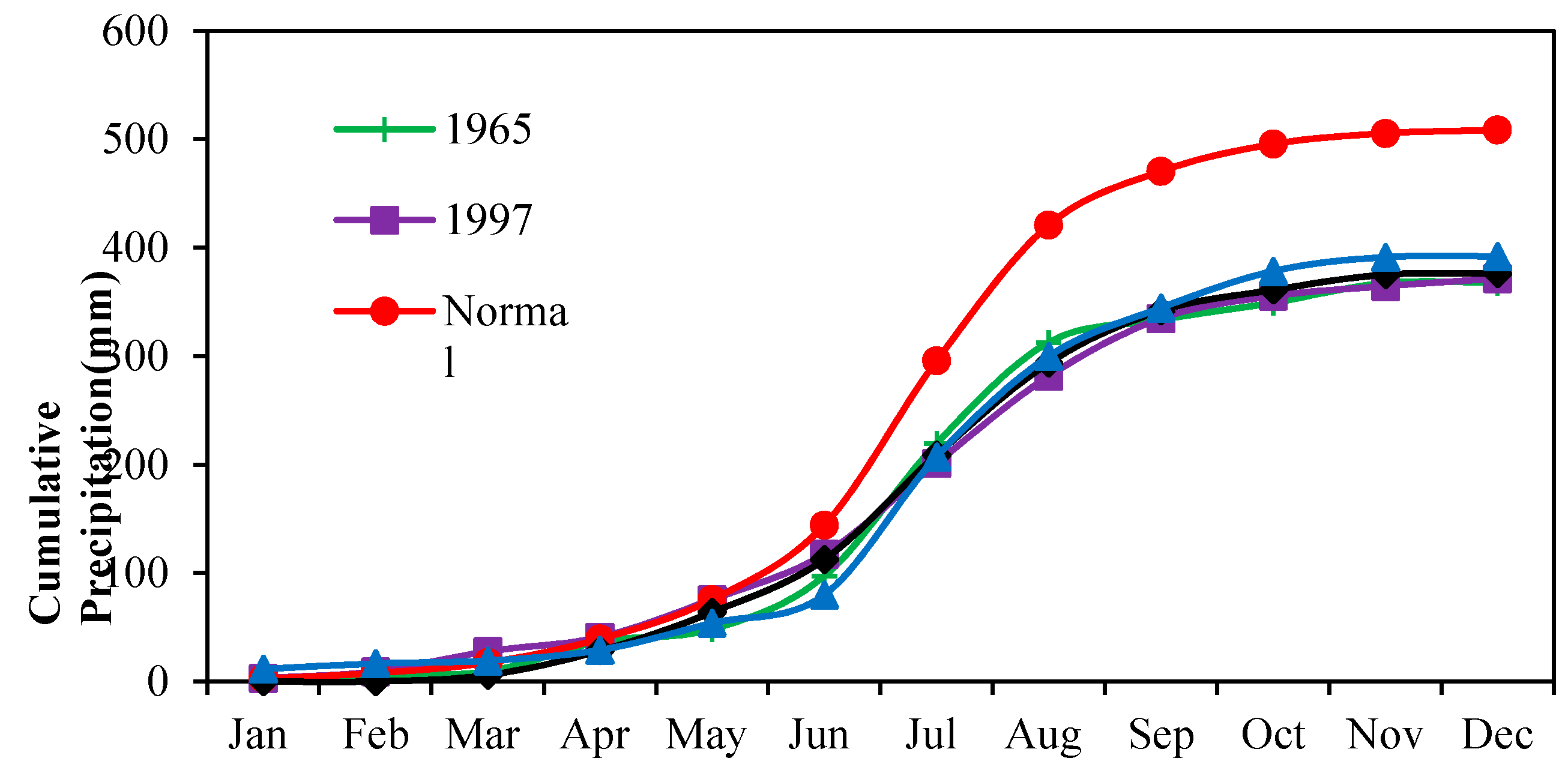
2. Study Area and Database

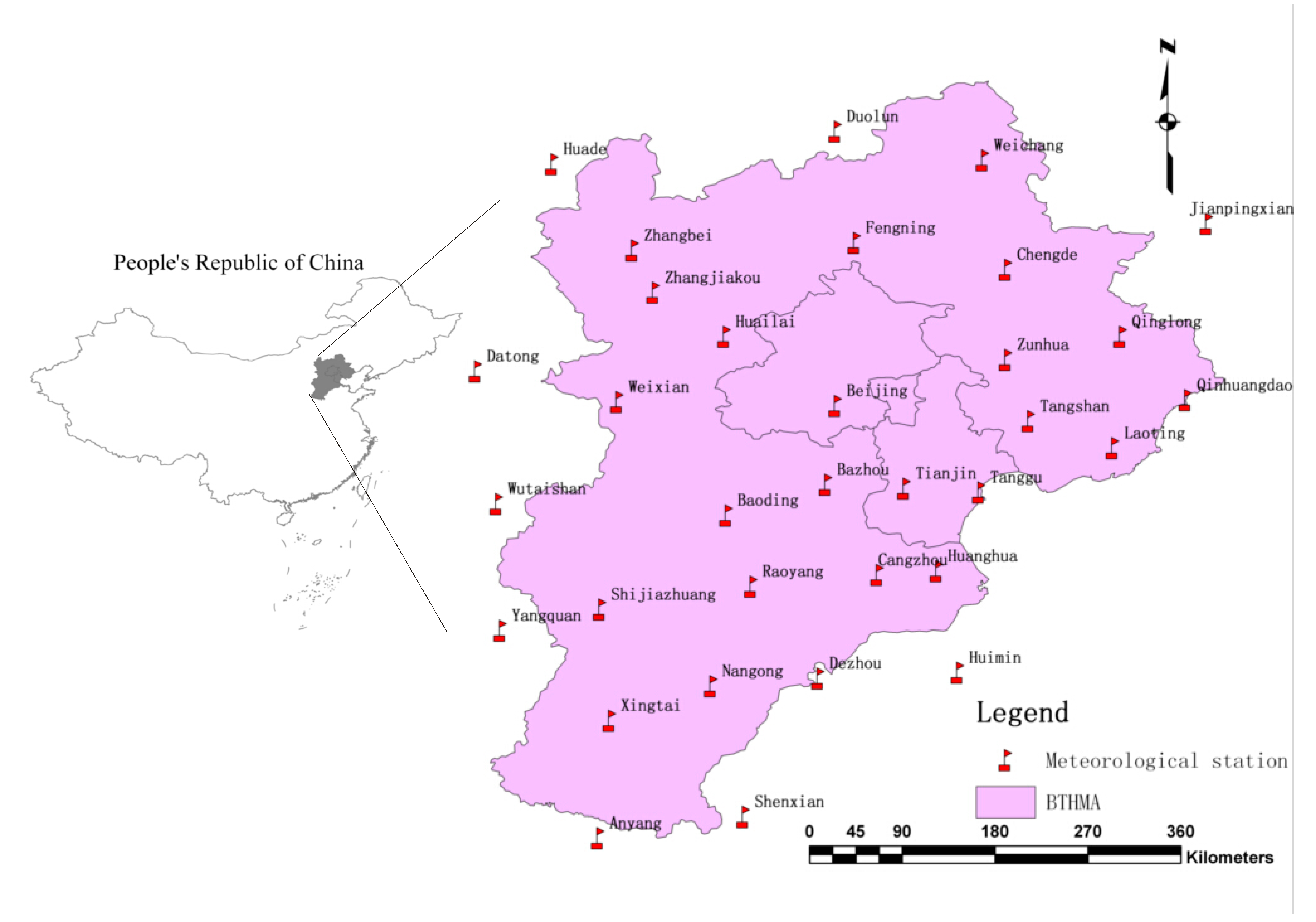
The study area is the Beijing-Tianjin-Hebei Metropolitan area located in north of North China Plain (Figure 1). The region, which encompasses China’s northernmost metropolitan region andits major cities, Beijing and Tianjin, is located in Hebei province and stretches from the municipalities of Beijing and Tianjin towards the Bohai Sea. The BTHMA is a plain region surrounded by the Yanshan Mountains in the north and the Taihang Mountains in the west, the coast of the Bohai Sea in the east, the North China Plain in the south, and the Inner Mongolia Plateau in the northwest. The BTHMA’s total area is roughly 185,000 km². The elevation ranges from sea level at the eastern coastal area to more than 2208 m at the northern and western mountain areas, and the mean elevation of the region is nearly 404.96 m (Table 1).

In the BTHMA the climate is continental; the springs are droughty, the summers are hot and the winters are cold, and the temperature difference between the summer and the winter is large. Summers in the BTHMA are usually very hot and wet, and in July and August temperatures can reach 40 °C. Mean annual precipitation over the whole BTHMA is about 519 mm and it is distributed unevenly in space and time. The mean annual precipitation varies from about 400 mm at the southern plain area to more than 1180 mm at the western mountain peaks. Generally, the maximum precipitation occurs in July and August, and the minimum in February. The northern mountain areas receive significant amounts of snow during the winter months and transient snowpack develop.

Table 1. Geographical descriptions mean and standard deviation of annual precipitation time series of the synoptic stations used in the study.

Station Name	Longitude (E)	Latitude (N)	Elevation (m)	Mean (mm)	Standard Deviation (mm)
Beijing	116.47	39.80	31.30	536.32	172.07
Zhangbei	114.70	41.15	1393.30	386.94	68.47
Weixian	114.57	39.83	909.50	398.88	88.09
Shijiazhuang	114.42	38.03	81.00	525.89	172.28
Xingtai	114.50	37.07	77.30	515.19	176.86
Fengning	116.63	41.22	661.20	458.04	89.55
Weichang	117.75	41.93	842.80	433.49	88.21
Zhangjiakou	114.88	40.78	724.20	399.00	91.85
Huailai	115.50	40.40	536.80	378.98	80.58
Chengde	117.95	40.98	385.90	518.28	108.71
Zunhua	117.95	40.20	54.90	711.88	201.17
Qinglong	118.95	40.40	227.50	691.79	190.63
Qinhuangdao	119.52	39.85	2.40	634.01	179.22
Bazhou	116.38	39.12	9.00	511.18	184.55
Tangshan	118.15	39.67	27.80	605.37	160.43
Laoting	118.88	39.43	10.50	600.22	176.73
Baoding	115.52	38.85	17.20	517.57	195.07
Raoyang	115.73	38.23	19.00	519.99	153.49
Cangzhou	116.83	38.33	9.60	610.09	194.76
Huanghua	117.35	38.37	6.60	589.70	196.37
Nangong	115.38	37.37	27.40	478.54	142.07
Anyang	114.40	36.05	62.90	561.60	169.20
Jianpingxian	119.70	41.38	422.00	459.86	107.01
Huade	114.00	41.90	1482.70	307.79	66.02
Duolun	116.47	42.18	1245.40	375.24	70.05
Dezhou	116.32	37.43	21.20	567.40	182.87
Huimin	117.53	37.48	11.70	572.64	172.16
Shenxian	115.67	36.23	37.80	539.63	158.65
Datong	113.33	40.10	1067.20	370.24	84.31
Wutaishan	113.52	38.95	2208.30	748.29	183.55
Yangquan	113.55	37.85	741.90	541.07	148.24
Tianjin	117.07	39.08	2.50	536.45	147.41
Tanggu	117.72	39.05	4.80	575.59	183.33

Table 1. Geographical descriptions mean and standard deviation of annual precipitation time series of the synoptic stations used in the study.

Station Name	Longitude (E)	Latitude (N)	Elevation (m)	Mean (mm)	Standard Deviation (mm)
Beijing	116.47	39.80	31.30	536.32	172.07
Zhangbei	114.70	41.15	1393.30	386.94	68.47
Weixian	114.57	39.83	909.50	398.88	88.09
Shijiazhuang	114.42	38.03	81.00	525.89	172.28
Xingtai	114.50	37.07	77.30	515.19	176.86
Fengning	116.63	41.22	661.20	458.04	89.55
Weichang	117.75	41.93	842.80	433.49	88.21
Zhangjiakou	114.88	40.78	724.20	399.00	91.85
Huailai	115.50	40.40	536.80	378.98	80.58
Chengde	117.95	40.98	385.90	518.28	108.71
Zunhua	117.95	40.20	54.90	711.88	201.17
Qinglong	118.95	40.40	227.50	691.79	190.63
Qinhuangdao	119.52	39.85	2.40	634.01	179.22
Bazhou	116.38	39.12	9.00	511.18	184.55
Tangshan	118.15	39.67	27.80	605.37	160.43
Laoting	118.88	39.43	10.50	600.22	176.73
Baoding	115.52	38.85	17.20	517.57	195.07
Raoyang	115.73	38.23	19.00	519.99	153.49
Cangzhou	116.83	38.33	9.60	610.09	194.76
Huanghua	117.35	38.37	6.60	589.70	196.37
Nangong	115.38	37.37	27.40	478.54	142.07
Anyang	114.40	36.05	62.90	561.60	169.20
Jianpingxian	119.70	41.38	422.00	459.86	107.01
Huade	114.00	41.90	1482.70	307.79	66.02
Duolun	116.47	42.18	1245.40	375.24	70.05
Dezhou	116.32	37.43	21.20	567.40	182.87
Huimin	117.53	37.48	11.70	572.64	172.16
Shenxian	115.67	36.23	37.80	539.63	158.65
Datong	113.33	40.10	1067.20	370.24	84.31
Wutaishan	113.52	38.95	2208.30	748.29	183.55
Yangquan	113.55	37.85	741.90	541.07	148.24
Tianjin	117.07	39.08	2.50	536.45	147.41
Tanggu	117.72	39.05	4.80	575.59	183.33

Figure 1. Spatial distribution of the 33 meteorological stations in Beijing-Tianjin-Hebei Metropolitan area map.

Figure 1. Spatial distribution of the 33 meteorological stations in Beijing-Tianjin-Hebei Metropolitan area map.

BTHMA experienced severe, extreme and persistent droughts during the period from mid 1960s to early 1970s and the period from late 1990s to early 2000s. The average cumulative areal precipitation during these two periods is compared to normal cumulative areal precipitation in Figure 2. During these two periods the monthly and annual precipitation were significantly below normal. In particular, 1965 and 1997 were the first and second driest years on record, respectively (Figure 2).

The driest January and February and the second driest December in record occurred in 1965. The prolonged and significant decrease of monthly and annual precipitation had a dramatic impact on water resources of the region. Usually, the dry periods are accompanied by high temperatures, which lead to higher evapotranspiration rates and dry soils [32]. These conditions inversely affect both the natural vegetation and the agriculture of the region as well as the available storage of the reservoirs. Severe and extremely dry conditions result in irrigation cutbacks, overexploitation of groundwater and significant losses of crop yields.

The estimation of the RDI values was based on monthly precipitation data and the potential evapotranspiration (PET). Monthly precipitation data and temperature data from 33 stations distributed over the BTHMA (Figure 1 and Table 1) and for the 1960 to 2010 period were available. The locations of the stations are shown in Figure 1. The elevation of these stations ranges from 2.4 m to 2208.3 m (Table 1). These precipitation data were used for the spatial distribution of monthly precipitation over the BTHMA as discussed in the next section of the paper.

Figure 2. Cumulative areal precipitation for selected dry years.

Figure 2. Cumulative areal precipitation for selected dry years.

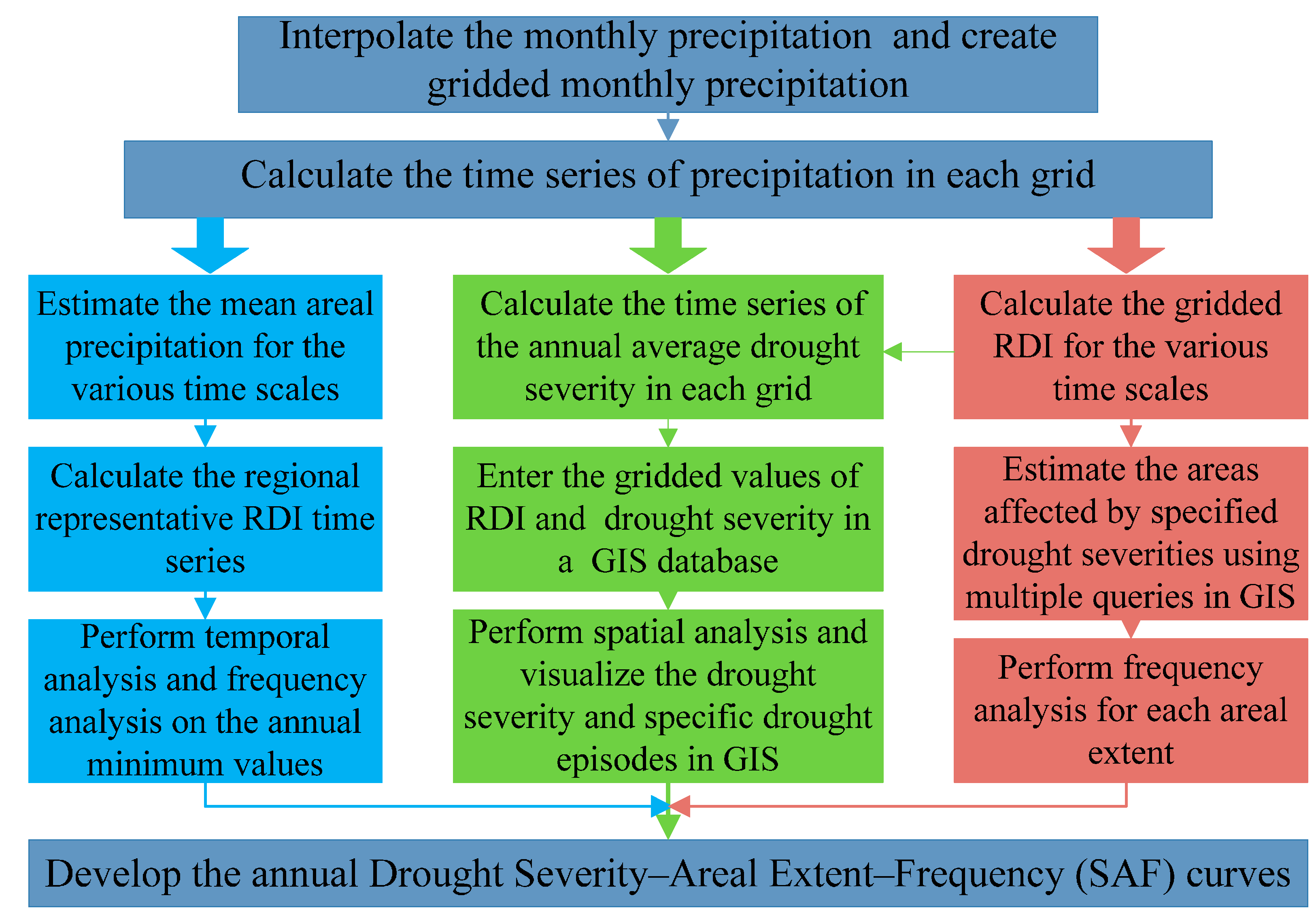
3. Materials and Methods

The methodology presented in this paper and applied to the BTHMA is as follows: the spatial interpolation of precipitation gauge data and the generation of gridded precipitation data; the calculation of the RDI values for each grid using the respective gridded precipitation for multiple timescales; analysis of the temporal characteristics of droughts in the BTHMA followed by the analysis of spatial characteristics of droughts in the BTHMA; and the development of drought severity-areal extent-frequency curves for the region for mean annual droughts and multiple time-scales. The steps in the methodology are shown in Figure 3.

Figure 3. The steps in the methodology.

Figure 3. The steps in the methodology.

In this study, the Geographical Information System(ArcGIS 10.0) was used for its ability to produce maps showing the spatial distribution of the RDI and, once the maps are produced, to answer multiple queries about the areas (or grids) with a specified value or range of values for the RDI. This ability is based on the connection of the GIS with the developed RDI database.

3.1. Spatial Interpolation of Precipitation

The spatial interpolation of precipitation over the BTHMA was estimated using a simple Multiple Linear Regression (MLR) model proposed by Naoum and Tsanis [33]. The general form of the model is:

P=a+b₁·X+b₂·Y+b₃·Z+b₄·X²+b₅·Y²+b₆·Z²+b₇·X·Y+b₈·X·Z+b₉·Y·Z

where P is the precipitation (mm), X is the longitude (km), Y is the latitude (km), Z is the elevation (m).

This MLR model was developed using stepwise linear regression. Terms of higher order only marginally improve the precipitation interpolation accuracy, leading, however, to spurious correlation between the interpolated and observed precipitation.

This MLR model was used because it yields realistic spatial distribution of precipitation, it provides reasonable estimates of areal precipitation for different scales, it is not greatly influenced by the number and the spatial distribution of precipitation gauges when estimating mean areal precipitation and its spatial distribution, and it is simple to apply. This model has been applied in Crete [33] for annual precipitation and its results were comparable with other spatial interpolation methods (likesplines, ordinary kriging, inverse distance weighting, and trend surface). Furthermore, Bostan et al.(2012) [34] compared five different statistical methods to spatially predict the average annual precipitation of Turkey using point observations of annual precipitation at meteorological stations and spatially exhaustive covariate data (i.e., elevation, aspect, surface roughness, distance to coast, land use and eco-region). The methods compared were multiple linear regression (MLR), ordinary kriging (OK), regression kriging (RK), universal kriging (UK), and geographically weighted regression (GWR).The results of all spatial interpolation methods were both cross-validated and independently validated and have shown that the simple MLR model gives reasonably good estimates of precipitation spatial distribution.

The MLR model was firstly calibrated using the monthly precipitation data from the 33 stations and its constants (a, b₁, b₂, …, b₉) were estimated for each month of the period 1960 to 2010. This means that 33 monthly MLR models were developed. The developed MLR models gave better results for the dry winter months than the wet summer months. This is expected due to the large spatial variation of precipitation during summer.

The MLR models were then applied to estimate the precipitation in grid cells with dimensions of 27 × 27 km and generate gridded precipitation for the period of 1960 to 2010. The total area of the BTHMA was divided into 253 grids and their elevation ranged from 2.4 m to 2208.3 m. Although these are large grids, they are suitable for drought analysis since droughts are regional phenomena affecting large areas. There are 146 county-level administrative units in the BTHMA, which are responsible for water resources management of their own district. Therefore, the 253 grid-cells were enough to demonstrate the drought of every county. Furthermore, the work presented in this paper is part of an ongoing research program. An objective of this research program is also to evaluate the forecasting potential of drought using, among others, remote sensing data, such as satellite vegetation indices (e.g., NDVI, Vegetation Condition Index (VCI)). Such remote sensing data are available, for the period of analysis, for grids 27 × 27 km, leading us to this selection of grid size.

3.2. Drought Identification

According to AsadiZarch et al. [35], the Reconnaissance Drought Index (RDI) was characterized as a general meteorological index for the drought assessment. The RDI is considered in three ways: the initial value (α_k), normalized RDI (RDI_n) and standardized RDI (RDI_st). The initial value (α_k) is presented in an aggregated form using a monthly time scale and may be calculated on a monthly, seasonal or annual basis. The α_k can be calculated usingthe following equation:

$${\alpha }_k^i=\frac{{\displaystyle {\sum }_{j=1}^k{P}_{ij}}}{{\displaystyle {\sum }_{j=1}^{12}PE{T}_{ij}}},i=1(1)Nandj=1(1)k$$

(1)

where P_ij and PET_ij are the precipitation and potential evapotranspiration within the month “j” of the year “i” and N is the total number of experimental years. Generally, the Penmann-Monteith equation is used to calculate PET; however, if required parameters are not available, it is recommended to use the Thornthwaite equation [36]. Suitability of the Thornthwaite equation has also been recommended in recent research works, e.g., [24,37]. Consequently, in the present research with limited data (only temperature), the Thornthwaite equation [38] was applied to calculate PET. Considering that using the selected PET methods has no significant influence on RDI, we selected the simplest Thornthwaite method [39].However, the temperature is corrected using the effective temperature instead of the mean. The effective temperature is defined as T_ef = 0.36 (3T_max − T_min).

Equation (1) could be calculated for any period of the year. It could also be recorded starting from any month of the year, if necessary. A second expression, the Normalized RDI (RDI_n) was computed using the following equation, in which it is evident that the parameter α_k is the arithmetic mean of α_k values.

$$RD{I}_n^{(i)}=\frac{{\alpha }_k^{(i)}}{{\stackrel{-}{\alpha }}_k}-1$$

(2)

The initial formulation of RDI_st [40] used the assumption that α_k values follow the log natural (ln) distribution. So, RDI_st was calculated as:

$$RD{I}_{\text{st}(k)}^{(i)}=\frac{y_k^{(i)}-\stackrel{-}{y_k}}{\stackrel{\wedge }{{\sigma }_{yk}}}$$

(3)

In which, yk is the ln (αk(i)), $\overline{y_k}$ was the arithmetic mean of yk and ${\widehat{\sigma }}_{yk}$ is the standard deviation. Based on an extended research on various data from several locations and different time scales, it was concluded that α_k values follow both the ln and the gamma distribution values at almost all locations and time scales. In most cases, though, the gamma distribution proved to be more successful.

According to Tsakiris et al. (2008) [41] and also Asadi Zarch et al. (2011) [35], it has been proved that the calculation of RDI_st could be performed better by fitting the gamma probability density function (pdf) to the given frequency distribution of α_k, following the procedure described below. Like SPI computation using the gamma approach, this method tends to solve the problem of calculating RDI_st for the small time scales, e.g., monthly, which may include zero precipitation values (α_k = 0), for which Equation (3) could not be applied [41]. The gamma distribution is defined by its frequency or probability density function:

$$g(x)=\frac{1}{{\beta }^{\alpha }\Gamma (\alpha )}{x}^{a-1}{e}^{-\raisebox{1ex}{$x$}\!\left/ \!\raisebox{-1ex}{$\beta $}\right.}for:x>0$$

(4)

where α > 0 is a shape factor; β > 0, a scale factor and x > 0 is the amount of precipitation [41]. Γ (α) is the gamma function, defined as:

$$\Gamma (\alpha )={\displaystyle {\int }_0^{\infty }{y}^{\alpha -1}{e}^{-y}dy}$$

(5)

Fitting of distribution to data requires the estimation of α and β as following:

$$\alpha \frac{1}{4A}\left(1+\sqrt{1+\frac{4A}{3}}\right)$$

(6)

$$\beta =\frac{\stackrel{\_}{x}}{\alpha }$$

(7)

where

$$A=\ln \left(\stackrel{\_}{x}\right)-\frac{1}{n}{\displaystyle \sum _{i=1}^n\ln (x_i)}$$

(8)

for n observations. The resulting parameters were then used to find the cumulative probability of an observed precipitation event for the given month or any other time scale:

$$G(x)={\displaystyle {\int }_0^{x}g(x)dx}=\frac{1}{{\beta }^{\alpha }\Gamma (\alpha )}{\displaystyle {\int }_0^x{x}^{a-1}{e}^{-\raisebox{1ex}{$x$}\!\left/ \!\raisebox{-1ex}{$\beta $}\right.}dx}$$

(9)

Substituting t for x_β reduces the Equation (6) to incomplete gamma function

$$G(x)=\frac{1}{\Gamma (\alpha )}{\displaystyle {\int }_0^x{t}^{\alpha -1}{e}^{-t}dt}$$

(10)

Since, the gamma function is undefined for x = 0 and a precipitation distribution may contain zeros, the cumulative probability becomes:

$$H(x)=q+(1-q)G(X)$$

(11)

where q is the probability of zero precipitation and G(X) is the cumulative probability of the incomplete gamma function. If m be the number of zeros in a α_k time scales, then q could be estimated by m/n. The cumulative probability H(x) is then transformed to the standard normal random variable z with mean zero and the variance of one [42], which is the value of RDI_st [43].

Positive values of RDI_st indicate wet periods, while negative values indicate dry periods compared with the normal conditions of the area. The severity of drought events increases when RDI_st values become negative. As per Dimitris Tigkas [31], we divided the RDI into moderate, severe and extreme classes for both dry and wet RDI as shown in Table 2.

In this study, the monthly gridded precipitation data were used for the estimation of the RDI for each grid cell for 3-month, 6-month and 12-month precipitation accumulations for each month of the period of analysis. The procedure, adopted in this study for the calculation of gridded RDI values, is called interpolate-calculate, because first the precipitation is spatially distributed, and then the RDI time series are calculated in each grid. An alternative strategy would be to firstly calculate the RDI time series at each precipitation station and then interpolate the RDI values into grids. This strategy is called calculate-interpolate. Bechini et al. (2000) [44] reported that the first procedure (i.e., interpolate-calculate procedure) should be followed, especially for non-linear models, paying considerable attention in the accurate interpolation of the initial parameters.

The calculation of drought indices performed through the software package Drought Indices Calculator (Drin C) [45,46], which was enhanced to meet the needs of this study.

Table 2. Drought classification of RDI.

Drought Class	RDI Value
Extremely wet	RDI ≥ 2.0
Very wet	1.5 ≤ RDI < 2.0
Moderately wet	1.0 ≤ RDI < 1.5
Near normal	−1.0 ≤ RDI < 1.0
Moderate drought	−1.5 ≤ RDI < −1.0
Severe drought	−2.0 ≤ RDI < −1.5
Extreme drought	RDI < −2.0

Table 2. Drought classification of RDI.

Drought Class	RDI Value
Extremely wet	RDI ≥ 2.0
Very wet	1.5 ≤ RDI < 2.0
Moderately wet	1.0 ≤ RDI < 1.5
Near normal	−1.0 ≤ RDI < 1.0
Moderate drought	−1.5 ≤ RDI < −1.0
Severe drought	−2.0 ≤ RDI < −1.5
Extreme drought	RDI < −2.0

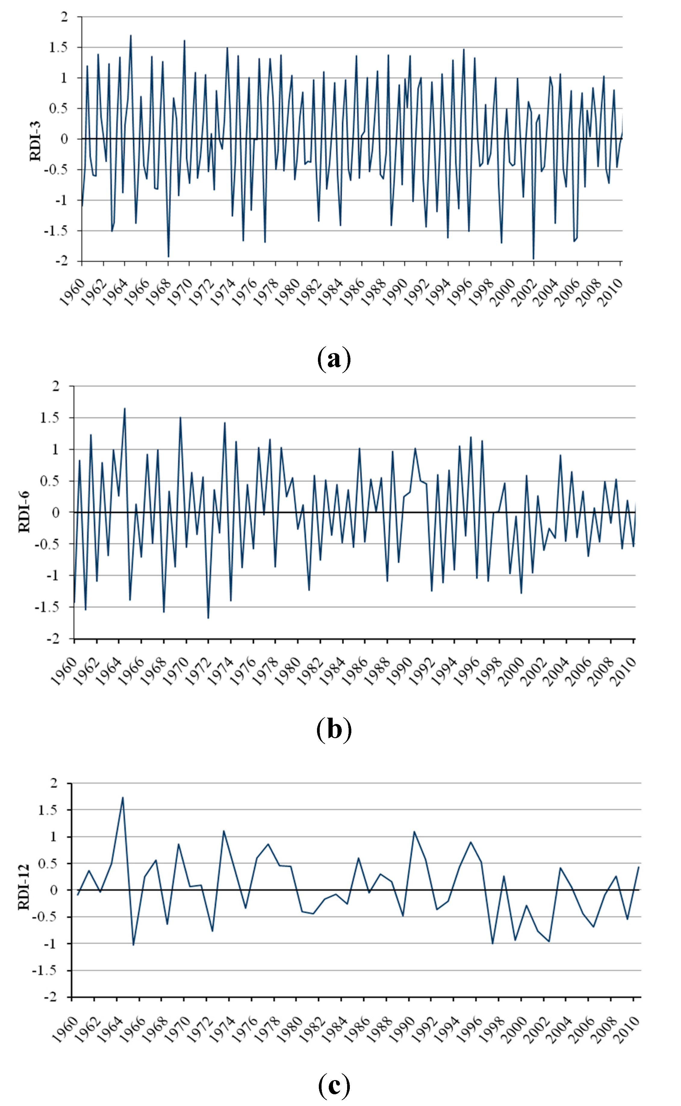
3.3. Temporal and Spatial Analysis of Droughts in the BTHMA

The temporal and spatial characteristics of droughts in the BTHMA were assessed by analyzing the gridded RDI values. The computed gridded RDI values of various time scales and for the period of analysis (1960 to 2010) were entered into a Geographical Information System (GIS) database. Firstly, the temporal variation of RDI was assessed using the regional representative of RDI, calculated from the time series of the mean areal precipitation of BTHMA. Analysis of the computed RDI time series revealed the most severe and extreme droughts occurred in the region. Then, the spatial characteristics of droughts during these severe dry periods were analyzed and visualized within the GIS. The spatial characteristics of droughts were further analyzed and the areas (or grids) affected by a specified drought severity were estimated within GIS. In this study, the inverse distance weighting(IDW)method was used for spatial interpolation and raster calculator was applied to calculate the area of drought. Finally, performing frequency analysis the annual drought intensity or drought severity-areal extent-frequency (SAF) curves were developed for the region.

The annual average SAF curves were developed according to the following procedure:

For every year, the computed gridded monthly RDI values for various time scales were used. The annual average drought severity in each grid was estimated by dividing the annual sum of RDI in monthly dry spells (negative RDI values) for a particular time scale by 12. Obtain the drought severity associated with the areal extent using the distribution map produced in the GIS. Perform frequency analysis for each drought areal extent percentage to associate the drought severity with return periods, considering an adequate probability distribution. Develop the average annual SAF curves for the particular time scale and repeat the analysis for the next timescale.

The frequency analysis is commonly used in hydrology and meteorology to assess the return period of particular events. In this study, the drought severity or drought intensity has negative values. The negative values of drought severity were transformed to positive values to represent extreme conditions and analyze the exceedance probability. Various theoretical probability distributions were statistically tested before fitting the observed drought severity. Specifically, the theoretical probability distributions tested for fitting the observed drought severity for the annual analyses (average annual drought severity) and for the various RDI time scales (3-month, 6-month and 12-month) were the Generalized Extreme Value (GEV), the Extreme Value I (EVI, Gumbel), Log-Normal-2 parameter, Log-Normal-3 parameter, Gamma, Log Pearson III, Generalized Pareto, and Weibull distributions. In this study, the non parametric Kolmogorov-Smirnov (K-S) test and the parametric Chi-Square test were used for the selection of the most adequate probability distribution, although other statistical tests may be applied, such as L-moments, L-skewness, and L-kurtosis. Most of the theoretical probability distributions tested (i.e., GEV, EVI, Gamma, Log Person III and Log- Normal-3 parameter) have passed the tests and could have been used for drought frequency analysis. However, the EVI distribution was selected for the analysis because (1) overall, it performed well for the annual and monthly analyses of drought severity and passed the two tests for all RDI time scales, (2) it is a two parameter probability distribution and its parameter values may be estimated with less uncertainty, especially for small samples, and (3) it is commonly used for drought analyses [47,48,49,50].

4. Results and Discussion

4.1. Temporal Characteristics of Droughts in BTHMA

The regional representative of RDI for the Beijing-Tianjin-Hebei Metropolitan area (BTHMA) was calculated for multiple time scales, using the mean areal precipitation (Figure 4). The analysis of the 3-month RDI and 6-month RDI time series indicated that the record minimum RDI observed in January 1968 and January 1972, respectively (Figure 4a and Figure 4b). The drought severity for both time scales was evaluated as severe (3-month RDI = −1.93 and 6-month RDI = −1.67) and had return periods of 14 and 20 years, respectively. The annual minimum RDI values for the 3-month and 6-month time scale most frequently occur during January and February (Table 3).

Table 3. Relative frequency of occurrence (%) of annual minimum monthly RDI for various time scales using regional representative RDI.

Month	3-Month RDI/%	6-Month RDI/%	12-Month RDI/%
January	21.5	19.8	12.8
February	16.1	19.8	16.1
March	12.5	12.5	21.1
April	9.1	9.1	9.2
May	3.2	5.8	5.2
June	3.2	3.1	3.1
July	6.3	0.0	3.1
August	6.3	3.1	3.0
September	3.2	5.8	5.2
October	6.3	6.1	6.3
November	9.1	5.8	6.3
December	3.2	9.1	9.8

Table 3. Relative frequency of occurrence (%) of annual minimum monthly RDI for various time scales using regional representative RDI.

Month	3-Month RDI/%	6-Month RDI/%	12-Month RDI/%
January	21.5	19.8	12.8
February	16.1	19.8	16.1
March	12.5	12.5	21.1
April	9.1	9.1	9.2
May	3.2	5.8	5.2
June	3.2	3.1	3.1
July	6.3	0.0	3.1
August	6.3	3.1	3.0
September	3.2	5.8	5.2
October	6.3	6.1	6.3
November	9.1	5.8	6.3
December	3.2	9.1	9.8

The annual minimum 12-month RDI values for the period of analysis were mainly observed in February and March (Table 3). Visual inspection of 12-month RDI time series (Figure 4c) indicated that droughts were quite frequent during the 1960s and the late1990s. However, two distinct severe dry periods were revealed, considering only the annual minimum spatially averaged RDI value. The first period occurred during the year 1965 and is characterized as a moderate drought event. The second period was the period from the year 1997 to 2002 and is characterized as a moderate drought for the whole BTHMA. Especially, the annual precipitation of the year 1965 is the smallest for the 51 years of analysis (1960 to 2010). The drought that occurred in 1965 is the most severe drought ever experienced in the BTHMA. The annual minimum 12-month RDI was observed in 1965 (RDI = −1.02) and had an estimated frequency of recurrence of 14 years.

Figure 4. Time series of average RDI values for the Beijing-Tianjin-Hebei Metropolitan area (BTHMA) for (a) 3-month, (b) 6-month and (c) 12-monthtime scales.

Figure 4. Time series of average RDI values for the Beijing-Tianjin-Hebei Metropolitan area (BTHMA) for (a) 3-month, (b) 6-month and (c) 12-monthtime scales.

The second drought event is a much more prolonged drought event than the drought event of 1965 and lasted over five years (1997–2002); it is interrupted by a wet 1998 and continued until the end of 2002. The minimum values of spatially averaged monthly RDI were observed during the year 1997 for the 12-month time scales, and it is characterized as a moderate drought event. The minimum 12-month RDI was estimated for 1997 (RDI = −1.01). This event had an estimated return period of 15 years for the 12-month time scale. This prolonged drought event caused exploding water demands and subsequent impacts in the BTHMA, in general.

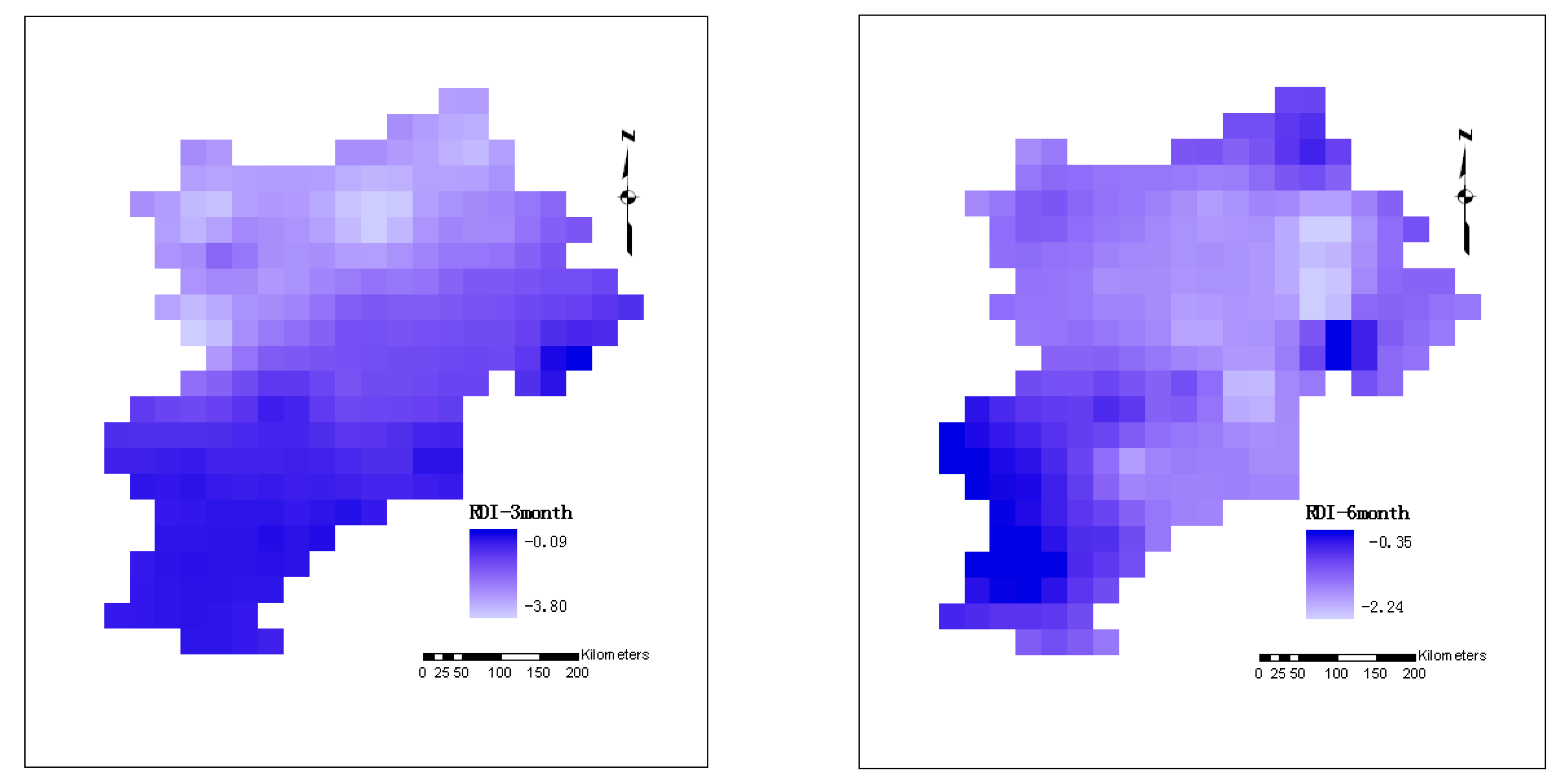
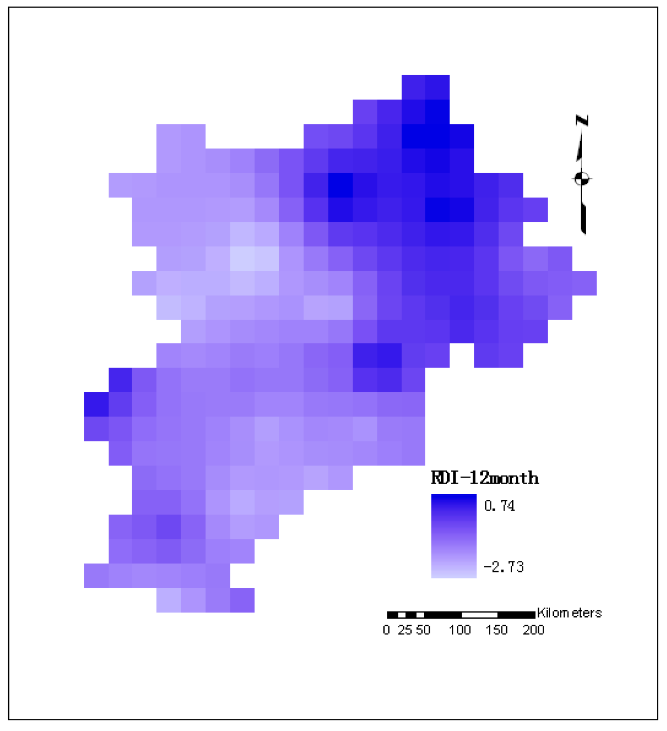
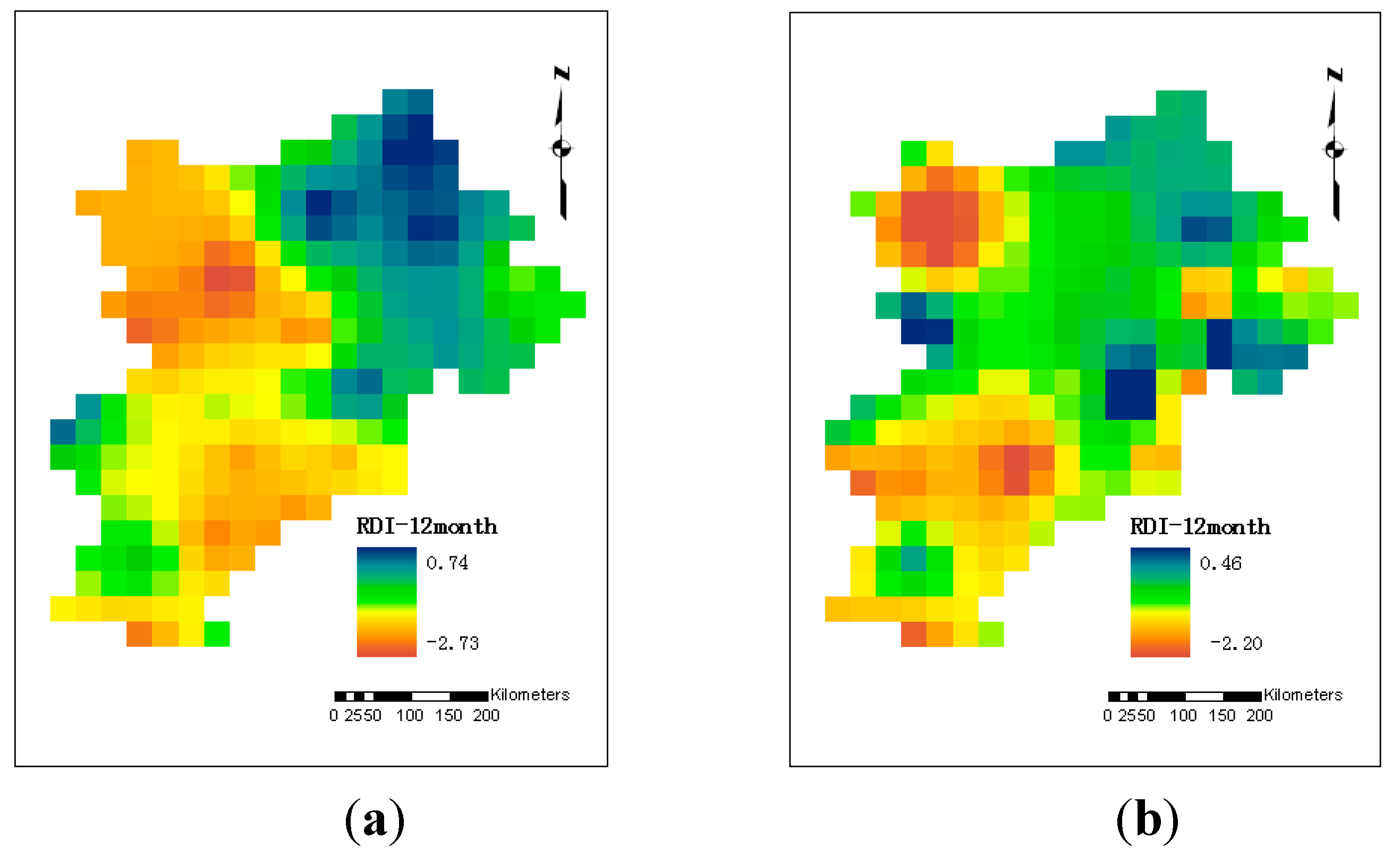
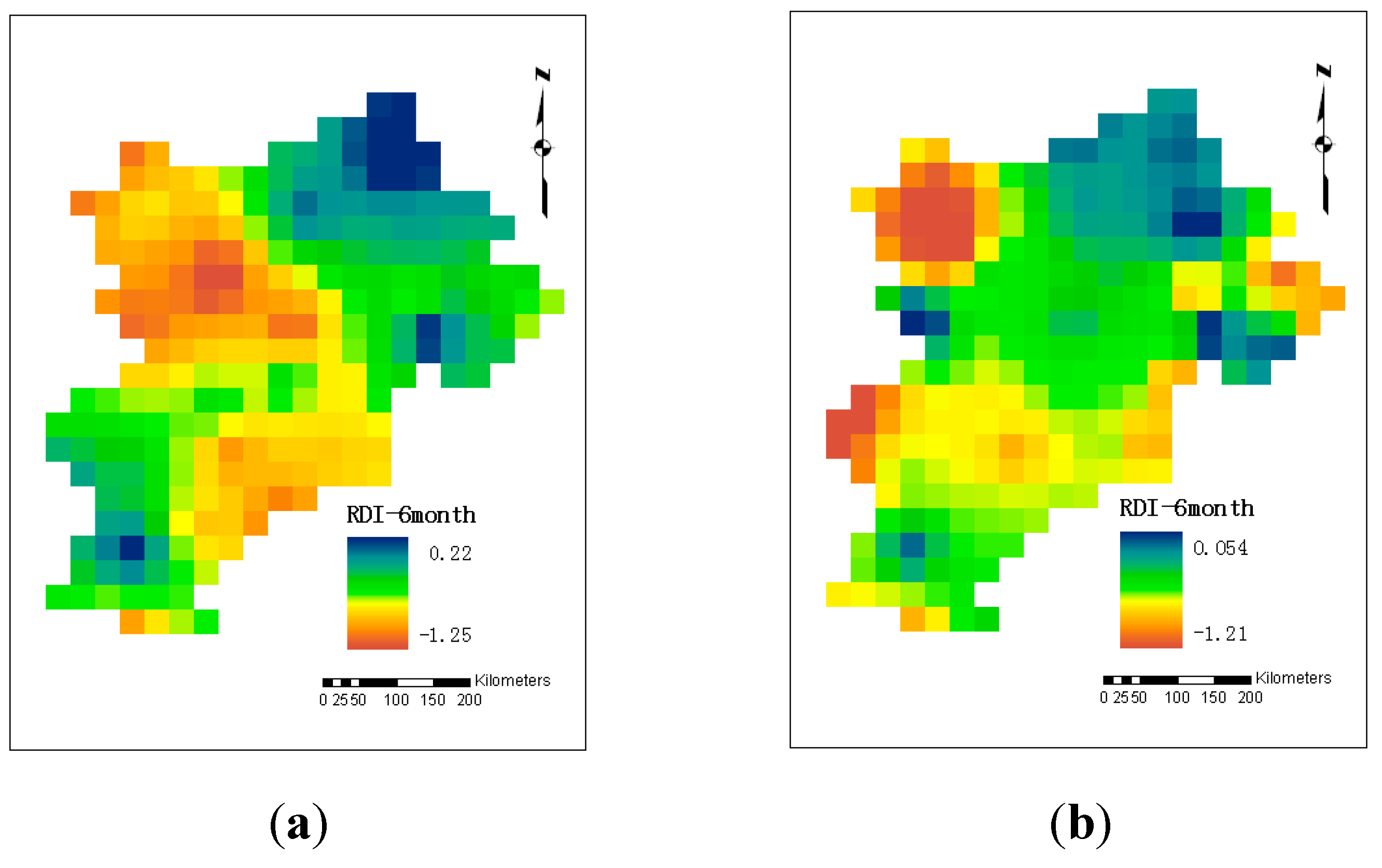
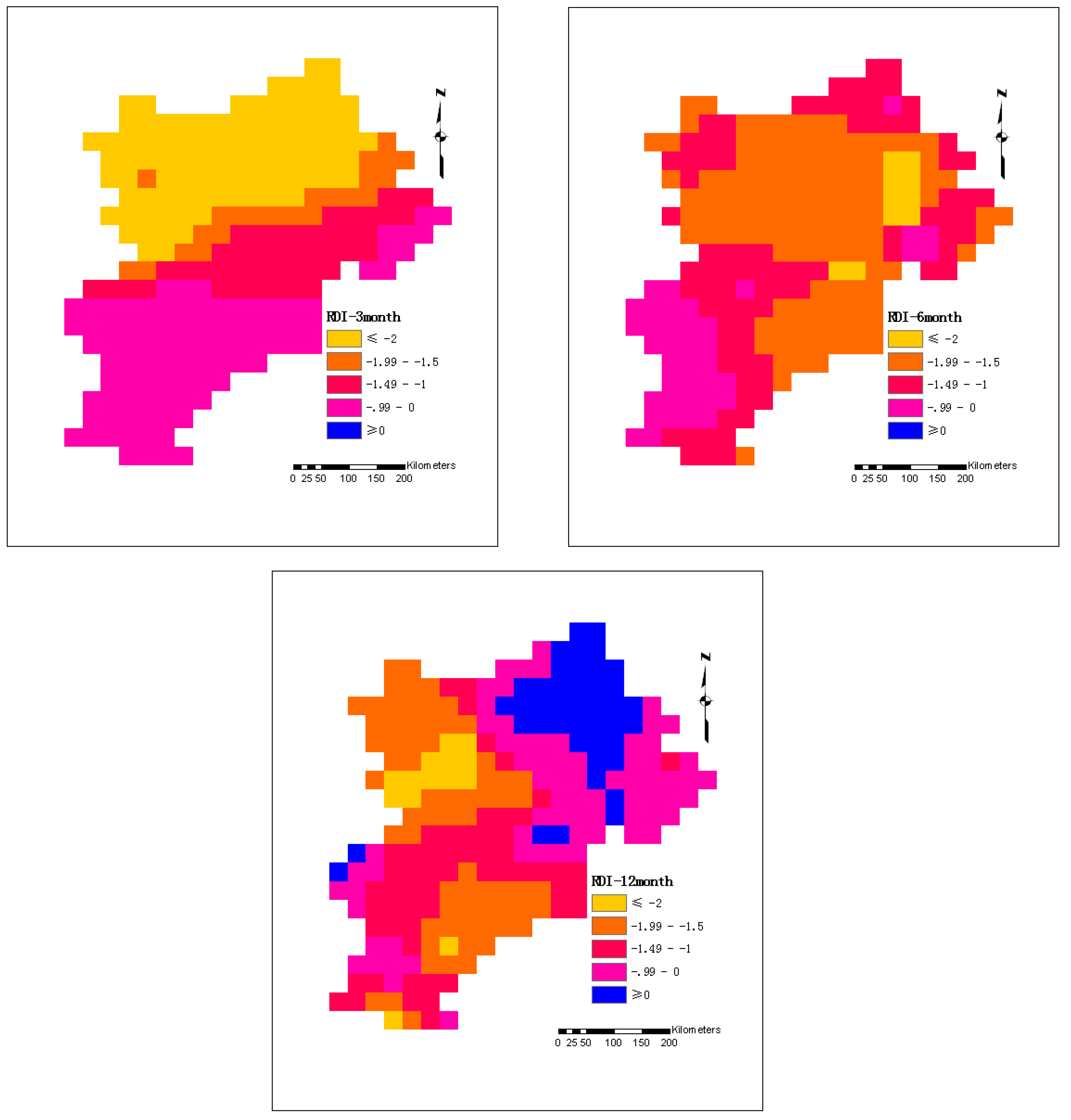
4.2. Spatial Characteristics of Droughts in the BTHMA

Although the estimation of drought severity at a point or as regionally representative gives useful information for water management, it is interesting and important to assess the drought over a specified region or basin. Regional drought analysis is useful for determining the spatial distribution and characteristics of drought, and evaluating the most affected areas for a specific drought event. In this study, the spatial analysis was performed using the gridded RDI values estimated for various time scales. Using the developed RDI database and the abilities of GIS, one can visualize the distribution of RDI values across the area of interest for various time scales. As an example, Figure 5 shows the variation of RDI across the BTHMA for 1965 for 3-month, 6-month and 12-monthtime scales. The spatial distribution of drought for this particular year is quite different when the RDI was assessed at the various time scales (Figure 5). Using the 3-month RDI, it seems that an area in the north of the region was the area most affected by the drought. When larger time scales of RDI are used (6-month), the pattern changes and indicates that the most drought-affected areas were the central areas of the region. Finally, the spatial variation of the 12-month RDI shows that the most affected areas were the western areas, which was consistent with former research [51].

Using GIS and the average annual RDI, the spatial distribution of a particular annual drought episode could be assessed. As an example, Figure 6 and Figure 7 show the spatial variation of the average annual 12-month and 6-month RDI, respectively, for the first (1965) and second (1997) driest years in record. Figure 6 indicates that during the year 1965, the average annual 12-month drought intensity was greater for the northwestern and some southeastern areas of the region, whereas during 1997 the most drought affected areas were in the northeastern and some central parts of the region. A similar spatial pattern was observed using the average annual 6-month RDI (Figure 7) for the years of 1965 and 1997.

The above analyses show that, when accounting the duration and the intensity of drought, indeed, the drought of the year 1965 was more severe than the drought of 1997. For example, the average annual 12-month RDI for 1965 and 1997 (Figure 6) ranges from −2.73 to 0.74, and −2.20 to 0.45, respectively. Similarly, the analysis for the average annual 6-month RDI (Figure 7) indicates that the RDI values for 1965 range from −1.25 to 0.22 whereas, the RDI for the latter year ranges from −1.21 to 0.05. These results also confirm the above analysis for the estimation of drought severity.

Figure 5. Variation of RDI in 1965 across BTHMA for various time scales.

Figure 5. Variation of RDI in 1965 across BTHMA for various time scales.

Figure 6. Spatial variations of average annual 12-month RDI for (a) the year 1965, and (b) the year 1997.

Figure 6. Spatial variations of average annual 12-month RDI for (a) the year 1965, and (b) the year 1997.

Figure 7. Spatial variations of average annual 6-month RDI for (a) the year 1965, and (b) the year 1997.

Figure 7. Spatial variations of average annual 6-month RDI for (a) the year 1965, and (b) the year 1997.

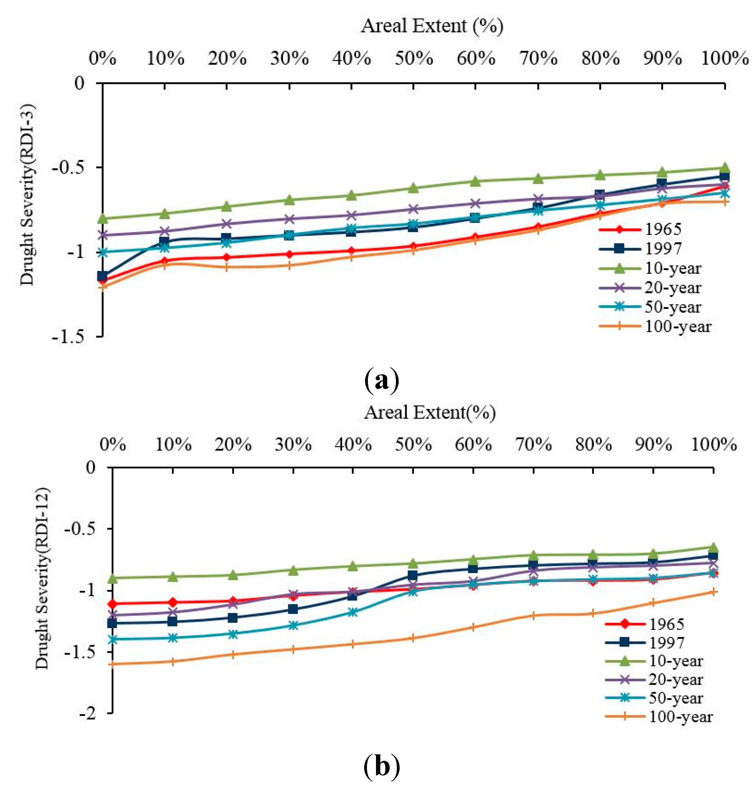
4.3. Drought Severity-Areal Extent-Frequency Curves for the BTHMA

A method to assess the spatial characteristics and the frequency over an area is drought severity-areal extent-frequency (SAF) curves. In this study, SAF curves were developed for the BTHMA using GIS capabilities and the spatial RDI database. The SAF curves were developed for the average annual drought severity for multiple time scales of RDI. The procedures for estimating the SAF curves have been outlined earlier in the paper. The percentage of the areal extent associated with a specified drought severity (or negative RDI value) was obtained by applying multiple queries in the GIS RDI database and analyzing the results. Figure 8 shows an example of such a multiple query for 1965. Since it is not feasible, due to paper length limitations, to show all the developed SAF curves, only indicative SAF curves will be presented.

Figure 8. Maps of areal extent for various time scales of RDI classes in 1965.

Figure 8. Maps of areal extent for various time scales of RDI classes in 1965.

Following the analysis steps previously presented, the SAF curves of the average annual drought severity were developed. Results were found in the analysis of the average annual SAF curves (Figure 9).These results indicate that the 1965 drought event was much more prolonged with continuous negative monthly values of RDI and had a negative impact on much larger area than the 1997 event. Thus, the drought that occurred in 1965 ear was more severe than the 1997 drought considering the duration and areal extent contrarily to the results of the analysis of the spatially averaged drought severity presented before.

Figure 9. Severity-areal extent-frequency curves of the average annual drought severity for (a) 3-month RDI, and (b) 12-month RDI.

Figure 9. Severity-areal extent-frequency curves of the average annual drought severity for (a) 3-month RDI, and (b) 12-month RDI.

5. Conclusions

This study was focused on presenting a framework of methodologies for the analysis of the temporal and spatial characteristics and frequency of droughts in the BTHMA in China. The RDI computed at various time scales was used as an indicator of drought severity. The RDI was computed using spatially distributed or gridded precipitation, and a database of computed RDI values was developed. Using this database, three analyses were performed: (1) an analysis of the temporal variation and frequency of droughts using the spatially averaged RDI over BTHMA as a regional representative, (2) an analysis of the spatial variation of droughts with the help of GIS capabilities, and (3) a regional frequency analysis that lead to the development of drought severity-areal extent-frequency curves. The last two analyses were performed for annual drought severity, and the annual drought severity was assessed by using the average annual negative RDI.

The temporal and spatial drought analyses indicated that the BTHMA experiences quite frequent moderate and severe droughts. The region experienced prolonged and severe droughts during the periods of 1965–1972 and 1997–2002. In particular, the persistent and prolonged drought of 1997–2002 seriously affected urban water supply and agricultural irrigation. The spatial variation of droughts during the two periods was quite different. For the 1965–1972 drought, the most affected areas were the northeastern and some western areas of BTHMA, whereas the northern and central areas of BTHMA were mostly affected during the prolonged drought during the period 1997–2002. It has been shown that the drought in the late 1990s was associated with a return period of more than 80 years with a large areal extent. The identification of the temporal and spatial characteristics of droughts in BTHMA will be useful for the development of a drought preparedness plan in the region.

Future research steps will be to investigate the interconnectivity of meteorological drought with hydrological and water resources drought, to evaluate the forecasting potential for droughts using meteorological data and remote sensing indices, and to predict the spatiotemporal distribution pattern of RDI with a generalized global interpolation model and drought forecasting modules in the future.

References

1. Wang, J.S.; Guo, J.Y.; Zhou, Y.W.; Yang, L.F. Progress and prospect on drought indices research. Arid Land Geogr. 2007, 30, 60–65. [Google Scholar]
2. Yao, Y.B.; Dong, A.X.; Wang, Y.R.; Zhang, X.Y.; Yang, J.H. Compare research of the regional arid characteristic base on Palmer drought severity index in spring over China. Arid Land Geogr. 2007, 30, 22–29. [Google Scholar]
3. Yu, W.J.; Shao, M.Y.; Ren, M.L.; Zhou, H.J.; Jiang, Z.H.; Li, D.L. Analysis on spatial and temporal characteristics drought of Yunnan Province. Acta Ecol. Sin. 2013, 33, 317–324. [Google Scholar] [CrossRef]
4. Yoo, J.; Kwon, H.H.; Kim, T.W.; Ahn, J.-H. Drought frequency analysis using cluster analysis and bivariate probability distribution. J. Hydrol. 2012, 420, 102–111. [Google Scholar] [CrossRef]
5. Sternberg, T. Regional drought has a global impact. Nature 2011, 472. [Google Scholar] [CrossRef]
6. Wilhite, D.A. Drought as a natural hazard: Concepts and definitions. In Drought: A Global Assessment; Wilhite, D.A., Ed.; Routledge: New York, NY, USA, 2000; pp. 3–18. [Google Scholar]
7. Paulo, A.A.; Rosa, R.D.; Pereira, L.S. Climate trends and behavior of drought indices based on precipitation and evapotranspiration in Portugal. Nat. Hazards Earth Syst. 2012, 12, 1481–1491. [Google Scholar] [CrossRef]
8. Gocic, M.; Trajkovic, S. Spatiotemporal characteristics of drought in Serbia. J. Hydrol. 2014, 510, 110–123. [Google Scholar] [CrossRef]
9. Liu, X.Y.; Li, D.L.; Wang, J.S. Spatiotemporal characteristics of drought over China during 1961–2009. J. Desert Res. 2012, 32, 473–483. [Google Scholar]
10. Li, S.Y.; Liu, R.H.; Shi, L.K.; Ma, Z.H. Analysis on drought characteristic of Henan in resent 40 years based on meteorological drought composite index. J. Arid Meteorol. 2009, 27, 97–102. [Google Scholar]
11. Bao, Y.X.; Meng, C.L.; Shen, S.H.; Qiu, X.F.; Gao, P.; Liu, C. Temporal and spatial patterns of droughts for recent 50 years in Jiangsu based on meteorological drought composite index. Acta Geogr. 2011, 66, 599–608. [Google Scholar]
12. Estrela, T.; Menendez, M.; Dimas, M.; Marcuello, C. Sustainable Water Use in Europe. Part 3: Extreme Hydrological Events: Floods and Droughts. Available online: http://www.eea.europa.eu/publications/Environmental_Issues_No_21 (accessed on 9 August 2001).
13. Yoo, C.; Kim, S. EOF analysis of surface soil moisture field variability. Adv. Water Resour. 2004, 27, 831–842. [Google Scholar] [CrossRef]
14. Clause, B.; Pearsonb, C.P. Regional frequency analysis of annual maximum streamflow drought. J. Hydrol. 1995, 173, 111–130. [Google Scholar] [CrossRef]
15. Yuan, G.F.; Wu, L.H. Spatial and temporal analysis on agricultural drought under double cropping system in Beijing-Tianjin-Hebei Plain area. Chin. J. Agrometeorol. 2000, 21, 5–9. [Google Scholar]
16. Yan, F.; Wang, Y.J.; Wu, B. Spatial and temporal distributions of drought in Hebei Province over the past 50 years. Geogr. Res. 2010, 39, 423–430. [Google Scholar]
17. Mishra, A.K.; Singh, V.P. A review of drought concepts. J. Hydrol. 2010, 354, 202–216. [Google Scholar] [CrossRef]
18. Dai, A. Characteristics and trends in various forms of the Palmer Drought Severity Index during 1900–2008. J. Geophys. Res. 2011, 116. [Google Scholar] [CrossRef]
19. Van Rooy, M.P. A rainfall anomaly index independent of time and space. Notos 1965, 14, 43–48. [Google Scholar]
20. Hollinger, S.E.; Isard, S.A.; Welford, M.R. A new soil moisture drought index for predicting crop yields. In Proceeding of 8th Conference on Applied Climatology, Anaheim, CA, USA, 17–22 January 1993.
21. Vasiliades, L.; Loukas, A.; Liberis, N. A water balance derived drought index for Pinios River Basin, Greece. Water Resources Manag. 2011, 25, 1087–1101. [Google Scholar] [CrossRef]
22. Palmer, W.C. Keeping track of crop moisture conditions, nationwide: The new crop moisture index. Weatherwise 1968, 21, 156–161. [Google Scholar] [CrossRef]
23. Gebrehiwot, T.; van der Veen, A.; Maathuis, B. Spatial and temporal assessment of drought in the Northern highlands of Ethiopia. Int. J. Appl. Earth Obs. Geoinf. 2011, 13, 309–321. [Google Scholar] [CrossRef]
24. Vangelis, H.; Tigkas, D.; Tsakiris, G. The effect of PET method on Reconnaissance Drought Index (RDI) calculation. J. Arid Environ. 2013, 88, 130–140. [Google Scholar] [CrossRef]
25. Heim, R.R., Jr. A review of twentieth-century drought indices used in the United States. Bull. Am. Meteorol. Soc. 2002, 83, 1149–1165. [Google Scholar] [CrossRef]
26. Asadi Zarch, M.A.; Sivakumar, B.; Sharma, A. Droughts in a Warming Climate: A Global Assessment of Standardized Precipitation Index (SPI) and Reconnaissance Drought Index (RDI). Available online: http://www.sciencedirect.com/science/article/pii/S002216941400763X (accessed on 5 October 2014).
27. Elagib, N.A.; Elhag, M.M. Major climate indicators of ongoing drought in Sudan. J. Hydrol. 2011, 409, 612–625. [Google Scholar] [CrossRef]
28. Farajalla, N.; Ziade, R. Drought Frequency under a Changing Climate in the Eastern Mediterranean: The Beka’a Valley, Lebanon. Available online: http://adsabs.harvard.edu/abs/2010EGUGA.1211653F (accessed on 29 October 2014).
29. Khalili, D.; Farnoud, T.; Jamshidi, H.; Kamgar-Haghighi, A.A.; Zand-Parsa, S. Comparability analyses of the SPI and RDI meteorological drought indices in different climatic zones. Water Resour. Manag. 2011, 25, 1737–1757. [Google Scholar] [CrossRef]
30. Kirono, D.G.C.; Kent, D.M.; Hennessy, K.J.; Mpelasoka, F. Characteristics of Australian droughts under enhanced greenhouse conditions: Results from 14 global climate models. J. Arid Environ. 2011, 75, 566–575. [Google Scholar] [CrossRef]
31. Dimitris, T.; Harris, V.; George, T. Drought and climatic change impact on streamflow in small watersheds. Sci. Total Environ. 2012, 440, 33–41. [Google Scholar] [CrossRef] [PubMed]
32. Ke, Z.; Kimball, J.S.; Kim, Y.W.; McDonald, K.C. Changing freeze-thaw seasons in northern high latitudes and associated influences on evapotranspiration. Hydrol. Process. 2011, 25, 4142–4151. [Google Scholar] [CrossRef]
33. Naoum, S.; Tsanis, I.K. Temporal and spatial variation of annual rainfall on the island of Crete, Greece. Hydrol. Process. 2003, 17, 1899–1922. [Google Scholar] [CrossRef]
34. Bostan, P.A.; Heuvelink, G.B.M.; Akyurek, S.Z. Comparison of regression and kriging techniques for mapping the average annual precipitation of Turkey. Int. J. Appl. Earth Observ. Geoinf. 2012, 19, 115–126. [Google Scholar] [CrossRef]
35. AsadiZarch, M.; Malekinezhad, H.; Mobin, M.; Dastorani, M.; Kousari, M. Drought monitoring by Reconnaissance Drought Index (RDI) in Iran. Water Resour. Manag. 2011, 25, 3485–3504. [Google Scholar] [CrossRef]
36. Droogers, P.; Allen, R.G. Estimating reference evapotranspiration under inaccurate data conditions. Irrig. Drain. Syst. 2002, 16, 33–45. [Google Scholar] [CrossRef]
37. Vangelis, H.; Spiliotis, M.; Tsakiris, G. Drought severity assessment based on bivariate probability analysis. Water Resour. Manag. 2011, 25, 357–371. [Google Scholar] [CrossRef]
38. Hargreaves, G.L.; Samani, Z.A. Reference crop evapotranspiration from temperature. Appl. Eng. Agr. 1985, 1, 96–99. [Google Scholar] [CrossRef]
39. Thornthwaite, C.W. An approach toward a rational classification of climate. Geogr. Rev. 1948, 38, 55–94. [Google Scholar] [CrossRef]
40. Tsakiris, G.; Vangelis, H. Establishing a drought index incorporating evapotranspiration. Eur. Water. 2005, 9, 3–11. [Google Scholar]
41. Tsakiris, G.; Nalbantis, I.; Pangalou, D.; Tigkas, D.; Vangelis, H. Drought Meteorological Monitoring Network Design for the Reconnaissance Drought Index (RDI). Available online: http://ressources.ciheam.org/om/pdf/a80/00800419.pdf (accessed on 29 October 2014).
42. Abramowitz, M.; Stegun, I.A. Handbook of mathematical functions: With formulas, graphs, and mathematical tables. In Applied Mathematics Series-55; Courier Corporation: Washington, DC, USA, 1965. [Google Scholar]
43. Kousari, M.R.; Dastorani, M.T.; Niazi, Y.; Soheili, E.; Hayatzadeh, M.; Chezgi, J. Trend detection of drought in arid and semi-arid regions of Iran based on implementation of reconnaissance drought index (RDI) and application of non-parametrical statistical method. Water Resour. Manag. 2014, 28, 1857–1872. [Google Scholar] [CrossRef]
44. Bechini, L.; Ducco, G.; Donatelli, M.; Stein, A. Modelling interpolation and stochastic simulation in space and time of global solar radiation. Agr. Ecosyst. Environ. 2000, 81, 29–42. [Google Scholar] [CrossRef]
45. Tsakiris, G.; Tigkas, D.; Vangelis, H.; Pangalou, D. Regional drought identification and assessment. Case study in Crete. In Methods and Tools for Drought Analysis and Management; Springer: Berlin, Germany, 2007; pp. 169–191. [Google Scholar]
46. Tigkas, D. Drought characterisation and monitoring in regions of Greece. Eur. Water. 2008, 23–24, 29–39. [Google Scholar]
47. Loukas1, A.; Vasiliades, L. Probabilistic analysis of drought spatiotemporal characteristics in Thessaly region, Greece. Natl. Hazards Earth Syst. Sci. 2004, 4, 719–731. [Google Scholar] [CrossRef]
48. Gottschalk, L.; Perzyna, G. Low Flow Distribution along a River. Available online: https://www.itia.ntua.gr/hsj/redbooks/213/hysj_213_01_0000.pdf#page=43 (accessed on 29 October 2014).
49. Lana, X.; Burgueno, A. Spatial and temporal characterization of annual extreme droughts in Catalonia (Northern Spain). Int. J. Climatol. 1998, 18, 93–110. [Google Scholar] [CrossRef]
50. Henriques, A.G.; Santos, M.J.J. Regional drought distribution model. Phys. Chem. Earth B 1999, 24, 19–22. [Google Scholar] [CrossRef]
51. Cai, W.; Zhang, Y.; Chen, Q.; Yao, Y. Spatial Patterns and Temporal Variability of Drought in Beijing-Tianjin-Hebei Metropolitan Areas in China. Available online: http://www.hindawi.com/journals/amete/aa/289471/ (accessed on 29 October 2014).