
Precipitation Sensitivity to the Mean Radius of Drop Spectra: Comparison of Single- and Double-Moment Bulk Microphysical Schemes


Abstract
:1. Introduction
2. Description of the Cloud Model
2.1. General Model Characteristics
2.2. Initial State of the Atmosphere

2.3. Model Versions

| Hydrometeors | DX,min (mm) | DX,max (mm) |
|---|---|---|
| Cloud droplets | 0.0 | 0.2 |
| Raindrops | 0.2 | 10.0 |
| Ice crystals | 0.0 | 1.0 |
| Snow | 0.0 | 5.0 |
| Graupel | 0.0 | 5.0 |
| Frozen raindrops | 0.0 | 5.0 |
| Hail | 5.0 | 50.0 |
| Hydrometeors | N0X (m−4) |
|---|---|
| Snow | 3 × 10⁶ |
| Graupel | 1.1 × 10⁶ |
| Frozen raindrops | 4 × 10⁴ |
| Hail | 4 × 10⁴ |
2.4. Experiment Design

3. Model Results and Discussion
3.1. Model Results


3.2. Discussion
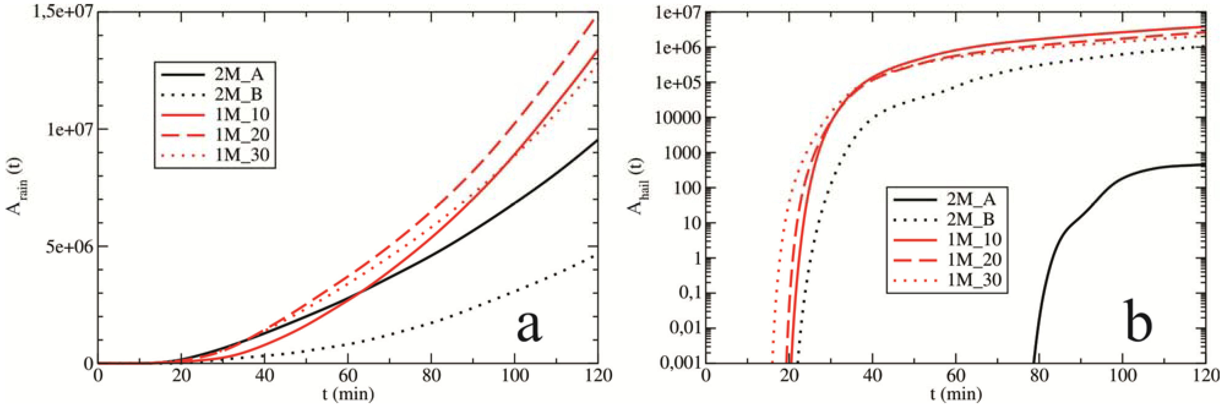
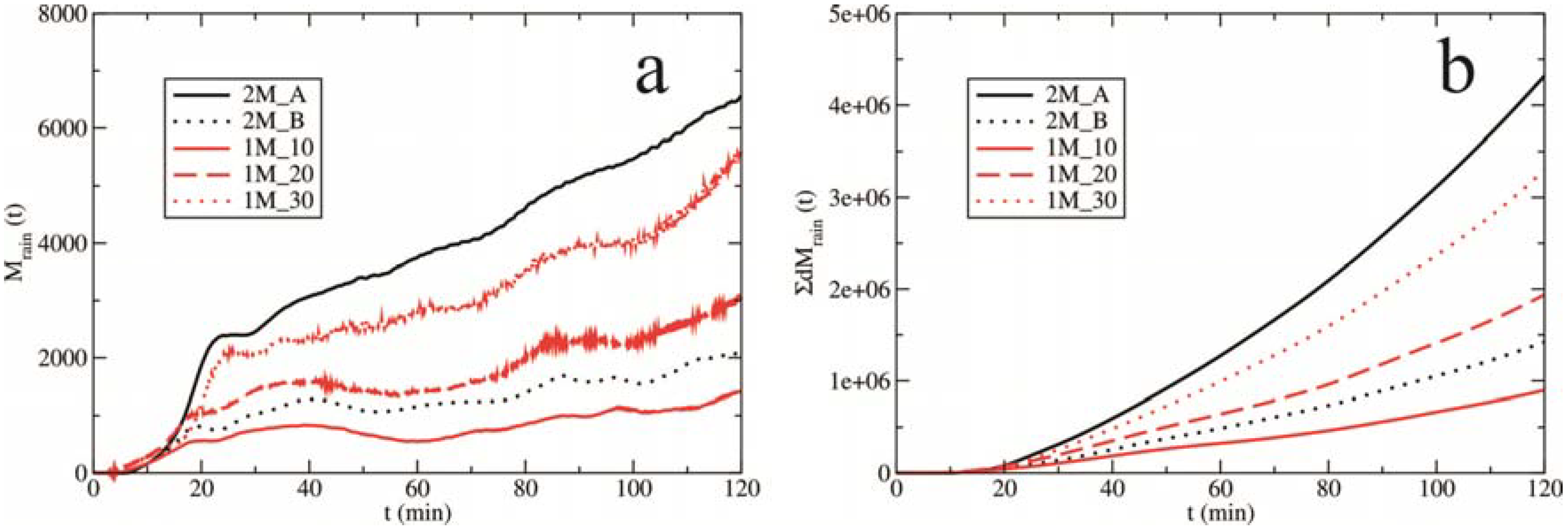
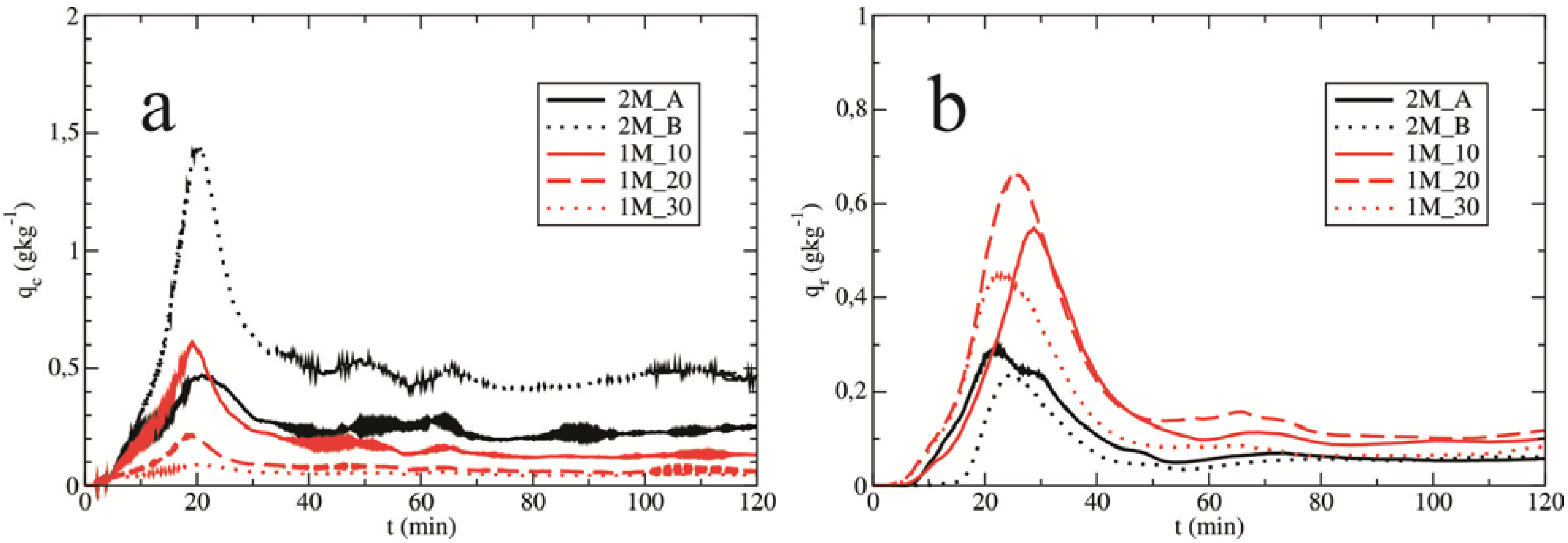
3.2.1. Rain


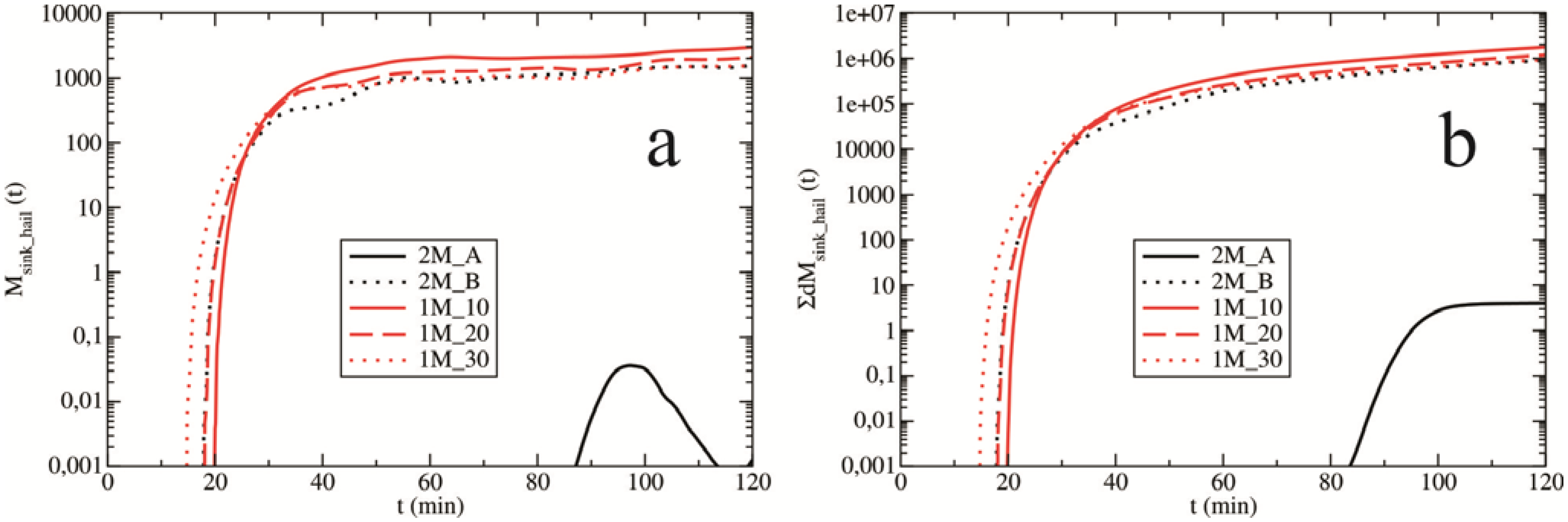
3.2.2. Hail


4. Conclusions
- The single-moment bulk microphysical scheme generates more surface rain than the double-moment scheme, particularly in the later stage of the cloud’s life. The cloud droplet number concentration increase (analogous to a decrease in the mean drop radius) leads to a large reduction in the accumulation of surface rain in the double-moment scheme. The single-moment scheme yields significantly more hail than the double-moment scheme.
- The double-moment scheme shows a much higher sensitivity of the amount and spatial distribution of the surface precipitation to the changing concentration of cloud droplets (or mean radius of the entire drop spectra) compared with the single-moment scheme.
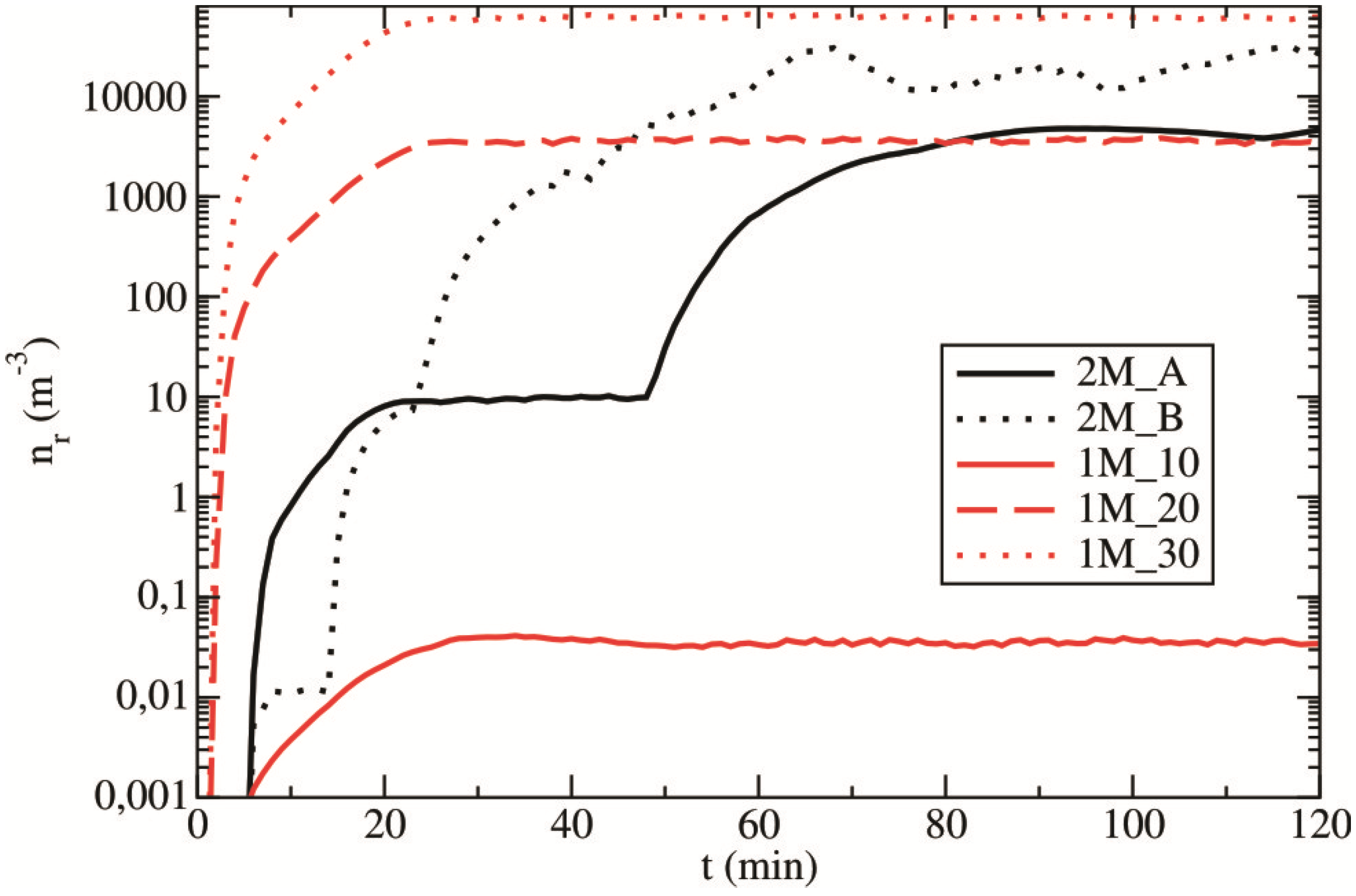
- The diagnostic rain concentration defined by the single-moment scheme may be unrealistic, i.e., underestimated or overestimated. In the case of very low rain concentrations, the accretion of cloud droplets (one of the primary processes in rain development) is insignificant. Nonetheless, the melting of precipitating ice is enormous, leading to a population of giant raindrops that is inconsistent with the observations. In the case with the single-moment scheme, large raindrops evaporate much faster compared with the population of smaller drops. Therefore, this scheme does not accurately simulate the evaporation of raindrops.
- In the sensitivity experiments generated by the double-moment scheme, there is a positive correlation between the increase in the cloud droplet number concentration and the size of the hail grains, consequently leading to an increase in hail production. Additionally, a higher cloud droplet number concentration leads to a greater mass of hail via pronounced riming. This cause-and-effect relationship is not observed in the single-moment experiments.
- The mean diameter of the hail, which is diagnostically determined by the single-moment scheme, is not consistent with the microphysical processes, such as the accretion rates, melting and sublimation of hailstones. Changing the mean radius of the drops has little impact on the mean diameters of the hailstones. An incorrect determination of the mean diameter of the hailstones by the single-moment scheme leads to an unrealistic description of microphysical processes.
- We strongly recommend using the double-moment bulk microphysical scheme with the unified Khrgian-Mazin size distribution for the entire drop spectrum. The prescribed value for the cloud droplet number concentration (or the mean radius of drops in the single-moment scheme) depends on the type of simulated cloud (maritime or continental). Therefore, the values of 60 and 600 cm−3 are recommended for the prescribed values of the cloud droplet number concentration in maritime and continental cases, respectively. Hence, the measurement of the cloud droplet number concentration can be very useful and substantial for numerical prediction of storms and theoretical considerations. If a cloud is simulated using the single-moment scheme, then a mean radius of 20 or 30 µm is appropriate for maritime convective clouds. Higher values of the mean radius of drops (e.g., 40 or 50 μm) are not observed [41]; therefore, these values are not recommended for simulating convective clouds with the single-moment scheme. The typical value of 10 µm for continental clouds [41] is not recommended due to the unrealistically small raindrop number concentration. Hence, we suggest using slightly higher values for the mean radius of drops (e.g., 15 μm).
Acknowledgments
Author Contributions
Conflicts of Interest
References
- Khain, A.; Rosenfeld, D.; Pokrovsky, A.; Blahak, U.; Ryzhkov, A. The role of CCN in precipitation and hail in a mid-latitude storm as seen in simulations using a spectral (bin) microphysics model in a 2D dynamic frame. Atmos. Res. 2011, 99, 129–146. [Google Scholar] [CrossRef]
- Sato, Y.; Nakajima, T.Y.; Nakajima, T. Investigation of the vertical structure of warm-cloud microphysical properties using the cloud evolution diagram, CFODD, simulated by a three-dimensional spectral bin microphysical model. J. Atmos. Sci. 2012, 69, 2012–2030. [Google Scholar] [CrossRef]
- Choi, I.-J.; Iguchi, T.; Kim, S.W.; Nakajima, T.; Yoon, S.C. The effect of aerosol representation on cloud microphysical properties in Northeast Asia. Meteorol. Atmos. Phys. 2014, 123, 181–194. [Google Scholar] [CrossRef]
- Rutledge, S.A.; Hobbs, P.V. The mesoscale and microscale structure and organization of clouds and precipitation in midlatitude Cyclones. XII: A diagnostic modeling study of precipitation development in narrow cold-frontal rainbands. J. Atmos. Sci. 1984, 41, 2949–2972. [Google Scholar] [CrossRef]
- Hu, Z.; He, G. Numerical simulation of microphysical processes in cumulonimbus—Part I: Microphysical model. Acta Meteorol. Sin. 1988, 2, 471–489. [Google Scholar]
- Murakami, M. Numerical modeling of dynamical and microphysical evolution of an isolated convective cloud—The 19 July 1981 CCOPE cloud. J. Meteorol. Soc. Jpn. 1990, 68, 107–127. [Google Scholar]
- Seifert, A.; Beheng, K.D. A two-moment cloud microphysics parameterization for mixed-phase clouds. Part I: Model description. Meteorol. Atmos. Phys. 2006, 92, 45–66. [Google Scholar] [CrossRef]
- Ćurić, M.; Janc, D.; Vučković, V.; Kovačević, N. The impact of the choice of the entire drop size distribution function on Cumulonimbus characteristics. Meteorol. Z. 2009, 18, 207–222. [Google Scholar] [CrossRef]
- Mansell, E.R.; Ziegler, C.L.; Bruning, E.C. Simulated electrification of a small thunderstorm with two-moment bulk microphysics. J. Atmos. Sci. 2010, 67, 171–194. [Google Scholar] [CrossRef]
- Grabowski, W.W.; Thouron, O.; Pinty, J.-P.; Brenguier, J.-L. A hybrid bulk-bin approach to model warm-rain processes. J. Atmos. Sci. 2010, 67, 385–399. [Google Scholar] [CrossRef]
- Onishi, R.; Takahashi, K. A warm-bin–cold-bulk hybrid cloud microphysical model. J. Atmos. Sci. 2012, 69, 1474–1497. [Google Scholar] [CrossRef]
- Lin, Y.-L.; Farley, R.D.; Orville, H.D. Bulk parameterization of the snow field in a cloud model. J. Appl. Meteorol. 1983, 22, 1065–1092. [Google Scholar] [CrossRef]
- Walko, R.L.; Cotton, W.R.; Meyers, M.P.; Harrington, J.Y. New RAMS cloud microphysics. Part I: The one moment scheme. Atmos. Res. 1995, 38, 29–62. [Google Scholar] [CrossRef]
- Xue, M.; Droegemeier, K.K.; Wong, V. The Advanced Regional Prediction System (ARPS)—A multi-scale nonhydrostatic atmospheric simulation and prediction model. Part I: Model dynamics and verification. Meteorol. Atmos. Phys. 2000, 75, 161–193. [Google Scholar] [CrossRef]
- Xue, M.; Droegemeier, K.K.; Wong, V.; Shapiro, A.; Brewster, K.; Carr, F.; Weber, D.; Liu, Y.; Wang, D. The Advanced Regional Prediction System (ARPS)—A multi-scale nonhydrostatic atmospheric simulation and prediction tool. Part II: Model physics and applications. Meteorol. Atmos. Phys. 2001, 76, 143–165. [Google Scholar] [CrossRef]
- Ćurić, M.; Janc, D.; Vučković, V. On the sensitivity of cloud microphysics under influence of cloud drop size distribution. Atmos. Res. 1998, 47–48, 1–14. [Google Scholar]
- Straka, J.M.; Mansell, E.R. A bulk microphysics parameterization with multiple ice precipitation categories. J. Appl. Meteorol. 2005, 44, 445–466. [Google Scholar] [CrossRef]
- Ferrier, B.S. A double-moment multiple-phase four-class bulk ice scheme. Part I: Description. J. Atmos. Sci. 1994, 51, 249–280. [Google Scholar] [CrossRef]
- Meyers, M.P.; Walko, R.L.; Harrington, J.Y.; Cotton, W.R. New RAMS cloud microphysics parameterization. Part II: The two-moment scheme. Atmos. Res. 1997, 45, 3–39. [Google Scholar] [CrossRef]
- Chen, B.; Xiao, H. Silver iodide seeding impact on the microphysics and dynamics of convective clouds in the high plains. Atmos. Res. 2010, 96, 186–207. [Google Scholar] [CrossRef]
- Kovačević, N.; Ćurić, M. The impact of the hailstone embryos on simulated surface precipitation. Atmos. Res. 2013, 132–133, 154–163. [Google Scholar]
- Kovačević, N.; Ćurić, M. Sensitivity study of the influence of cloud droplet concentration on hail suppression effectiveness. Meteorol. Atmos. Phys. 2014, 123, 195–207. [Google Scholar] [CrossRef]
- Milbrandt, J.A.; Yau, M.K. A multimoment bulk microphysics parameterization. Part II: A proposed three-moment closure and scheme description. J. Atmos. Sci. 2005, 62, 3065–3081. [Google Scholar] [CrossRef]
- Loftus, A.M.; Cotton, W.R. Examination of CCN impacts on hail in a simulated supercell storm with triple-moment hail bulk microphysics. Atmos. Res. 2014, 147–148, 183–204. [Google Scholar]
- Loftus, A.M.; Cotton, W.R.; Carrió, G.G. A triple-moment hail bulk microphysics scheme. Part I: Description and initial evaluation. Atmos. Res. 2014, 149, 35–57. [Google Scholar] [CrossRef]
- Ziemer, C.; Wacker, U. A comparative study of B-, Γ- and log-normal distributions in a three-moment parameterization for drop sedimentation. Atmosphere 2014, 5, 484–517. [Google Scholar] [CrossRef] [Green Version]
- Morrison, H.; Thompson, G.; Tatarskii, V. Impact of cloud microphysics on the development of trailing stratiform precipitation in a simulated squall line: Comparison of one- and two-moment schemes. Mon. Weather Rev. 2009, 137, 991–1007. [Google Scholar] [CrossRef]
- Molthan, A.L.; Colle, B.A. Comparisons of single- and double-moment microphysics schemes in the simulation of a synoptic-scale snowfall event. Mon. Weather Rev. 2012, 140, 2982–3002. [Google Scholar] [CrossRef]
- Van Weverberg, K.; Goudenhoofdt, E.; Blahak, U.; Brisson, E.; Demuzere, M.; Marbaix, P.; van Ypersele, J.-P. Comparison of one-moment and two-moment bulk microphysics for high-resolution climate simulations of intense precipitation. Atmos. Res. 2014, 147–148, 145–161. [Google Scholar] [CrossRef]
- Lim, K.-S.S.; Hong, S.-Y. Development of an effective double-moment cloud microphysics scheme with prognostic cloud condensation nuclei (CCN) for weather and climate models. Mon. Weather Rev. 2010, 138, 1587–1612. [Google Scholar] [CrossRef]
- Baba, Y.; Takahashi, K. Dependency of stratiform precipitation on a two-moment cloud microphysical scheme in mid-latitude squall line. Atmos. Res. 2014, 138, 394–413. [Google Scholar] [CrossRef]
- Tao, W.K.; Simpson, J.; McCumber, M. An ice-water saturation adjustment. Mon. Weather Rev. 1989, 117, 231–235. [Google Scholar] [CrossRef]
- Fletcher, N.H. The Physics of Rain Clouds; Cambridge University Press: Cambridge, UK, 1962; p. 390. [Google Scholar]
- Swann, H. Sensitivity to the representation of precipitating ice in CRM simulations of deep convection. Atmos. Res. 1998, 47–48, 415–435. [Google Scholar] [CrossRef]
- Ćurić, M. The development of the cumulonimbus clouds which moves along a valley. In Cloud Dynamics; D. Reidel Publishing Company: Dordrecht, The Netherlands, 1982; pp. 259–272. [Google Scholar]
- Ochou, A.D.; Nzeukou, A.; Sauvageot, H. Parametrization of drop size distribution with rain rate. Atmos. Res. 2007, 84, 58–66. [Google Scholar] [CrossRef]
- Pruppacher, H.R.; Klett, J.D. Microphysics of Clouds and Precipitation, 2nd ed.; Kluwer: Dordrecht, The Netherlands, 1997; p. 954. [Google Scholar]
- Abramowitz, M.; Stegun, I.A. Handbook of Mathematical Functions with Formulas, Graphs, and Mathematical Tables; Dover Publications: Mineola, NY, USA, 1970; p. 364. [Google Scholar]
- Gunn, K.L.S.; Marshall, J.S. The distribution with size of aggregate snowflakes. J. Meteorol. 1958, 15, 452–461. [Google Scholar] [CrossRef]
- Federer, B.; Waldvogel, A. Hail and raindrop size distributions from a Swiss multicell storm. J. Appl. Meteorol. 1975, 14, 91–97. [Google Scholar] [CrossRef]
- Wallace, J.M.; Hobbs, P.V. Atmospheric Science: An Introductory Survey, 2nd ed.; Academic Press: New York, NY, USA, 2006; p. 504. [Google Scholar]
- Niu, S.; Jia, X.; Sang, J.; Liu, X.; Lu, C.; Liu, Y. Distributions of raindrops sizes and fall velocities in a semiarid plateau climate: Convective versus stratiform rains. J. Appl. Meteorol. Clim. 2010, 49, 632–645. [Google Scholar] [CrossRef]
- Tang, Q.; Xiao, H.; Guo, C.; Feng, L. Characteristics of the raindrops size distributions and their retrieved polarimetric radar parameters in northern and southern China. Atmos. Res. 2014, 135–136, 59–75. [Google Scholar] [CrossRef]
© 2015 by the authors; licensee MDPI, Basel, Switzerland. This article is an open access article distributed under the terms and conditions of the Creative Commons Attribution license (http://creativecommons.org/licenses/by/4.0/).
Share and Cite
Kovačević, N.; Ćurić, M. Precipitation Sensitivity to the Mean Radius of Drop Spectra: Comparison of Single- and Double-Moment Bulk Microphysical Schemes. Atmosphere 2015, 6, 451-473. https://doi.org/10.3390/atmos6040451
Kovačević N, Ćurić M. Precipitation Sensitivity to the Mean Radius of Drop Spectra: Comparison of Single- and Double-Moment Bulk Microphysical Schemes. Atmosphere. 2015; 6(4):451-473. https://doi.org/10.3390/atmos6040451
Chicago/Turabian StyleKovačević, Nemanja, and Mladjen Ćurić. 2015. "Precipitation Sensitivity to the Mean Radius of Drop Spectra: Comparison of Single- and Double-Moment Bulk Microphysical Schemes" Atmosphere 6, no. 4: 451-473. https://doi.org/10.3390/atmos6040451