1. Introduction
Hydraulic conductivity, hence represented as K, is a very important aquifer parameter, because it measures how easily fluid flows through porous medias. Groundwater flow fields affect groundwater analyses, such as groundwater resource estimation, contamination transport, and heat transport. K most heavily influences groundwater flow fields. The more the amount of the K values, the better estimates are of the resulting groundwater flow fields, and consequently, the lower the uncertainty is of related groundwater analyses.
Although K is an important parameter for groundwater analysis, obtaining the actual K values is difficult. K values can vary over a large range even within the same type of soil/rock, and estimated values between the field tests and laboratory measurements are often different [
1,
2,
3]. In addition, the amount of K values from field pumping tests are limited due to the requirement of suitable lands, high cost of well installation, and long testing time for pumping tests [
2]. Due to these limitations, it is important to develop an efficient method for increasing the amount of K based on the limited pumping tests.
To increase the amount of K, a number of researchers [
2,
4,
5,
6,
7] have recently developed several methods to estimate K by integrating pumping tests data with surface electrical resistivity measurements. Some of these studies estimate K based on Archie’s law [
8]. Archie’s law, Equation (1), describes the relationship among bulk resistivity (
o), pore water resistivity (
w), saturation (S
w), saturation exponent (n), porosity (
), tortuosity factor (
), and cementation coefficient (m). Archie also proposes formation factor (F), defined in Equation (2), to describe the relationship among
,
and m:
For the saturated porous media,
, and Equation (2) can be can be modified to:
where
and
are different for sand, clay, and gravel [
9].
For Archie’s rock, its F value only varies with its rock structure, while for the sediment with clay, its F value varies with sediment composition/structure and pore water resistivity. This F value is called as apparent formation factor (
, see Equation (4)), and its parameters
and
vary with clay content, i.e., the increase in clay content results in the increase in
and decrease in
:
Apparent formation factor
removes the effect of pore water resistivity
and is related only to porosity
, tortuosity
, and cementation coefficient
factors. It is indicated in [
9] that
and
are different for sand, clay, and gravel. Since both F* and K are functions of porosity, the link between these two parameters can be developed through statistic regression.
Most previous studies applied Equation (4) to develop their K-F* mappings, and these mappings are then used to estimate their K fields. Their estimates are acceptable for their local aquifers, since the sediment compositions of a local aquifer may be similar [
2,
5,
6,
7,
10,
11]. However, for the groundwater system that consists of several alluvial fans (i.e., composite fan delta) with different geological formations, their proposed methods may not perform well since using a single K-F* mapping to fit all the K-F* relationships of the aquifers with different geological formations is difficult and unrealistic.
To efficiently and accurately estimate the spatial distribution of K for a groundwater system composed of the composite fan delta, this study proposes a method to integrate pumping test data and surface electrical resistivity measurements based on the data classification method. Here, we chose the Choushui River alluvial fan area in central Taiwan for showing the effectiveness of the method. First, the proposed methodology distinguishes the aquifers of the groundwater system into several zones based on the proposed zonation method, and all the data pairs are classified based on these given zones. Each zone’s sediment has similar characteristics, such as identical sediments source, aquifer type, etc. Next, each zone’s K-F* mapping equation is obtained by developing the regression equation of the F* and K data pairs. Finally, the K fields of all the aquifers are derived by using the developed K-F* mappings and kriging interpolation method.
2. Study Area
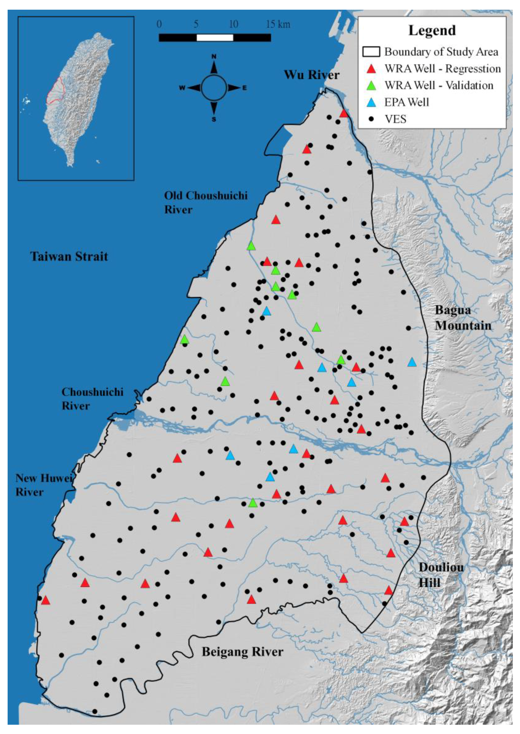
The Chuoshui River alluvial fan is located on the middle west of Taiwan and is bounded by the Wu River to the north, the Taiwan Strait to the west, the Beigang River to the south, and the Bagua Tableland to the east (
Figure 1).
The primary region of interest is the plain below 100 m in altitude; it covers approximately 2079 km2. The slope descends from the east to the west of the study area. There are five rivers flow through the entire study area and eventually reaches the Taiwan Strait. From north to south, the rivers are: the Wu, Old Chuoshui, Chuoshui, New Huwei, and Beigang River. The primary river of this area is the Chuoshui River.
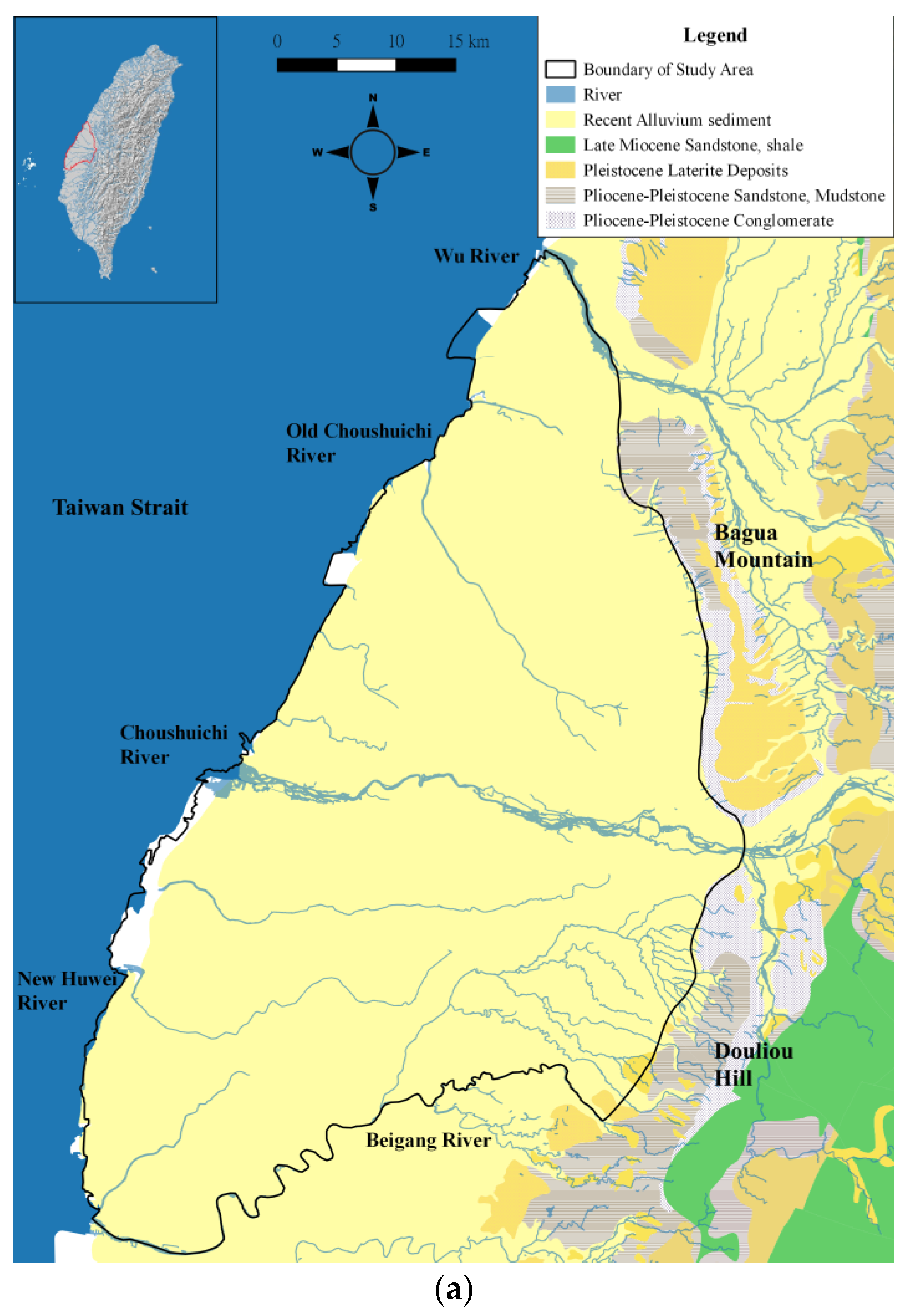
The surface of the Chuoshui River alluvial fan is covered by the Holocene alluvial sediments, which are unconsolidated sediments, mainly composed of gravel, sand, and mud. These sediments are distributed in the riverbed of the existing rivers, and the alluvial fans near the Bagua Tableland and the west side of the Douliu hills. This composite fan delta is mainly formed by the sediments from the Chuoshui River, Lugang River, Huwei River, and other east-west rivers, while the Douliu hills are mainly composed of the Pleistocene conglomerate facies, thick sandstone facies, and early Pleistocene fine-grained to silty layered sandstone. The Bagua Tableland is mainly composed of Pleistocene conglomerate facies and the late Pleistocene to the Holocene muddy gravel layers (
Figure 2a).
The sediments in the north boundary of the Chuoshui River alluvial fan are affected by the deposits sourced from Wu River, while the sediments in the south boundary of this fan are affected by the deposits sourced from the Beigang River. The sediments of the Beigang River consist of clay and sand that are sourced from the Douliou Hill, while the sediments of the Wu River are sand and gravel that are sourced from the Foothhill Mountain Range (
Figure 2a) [
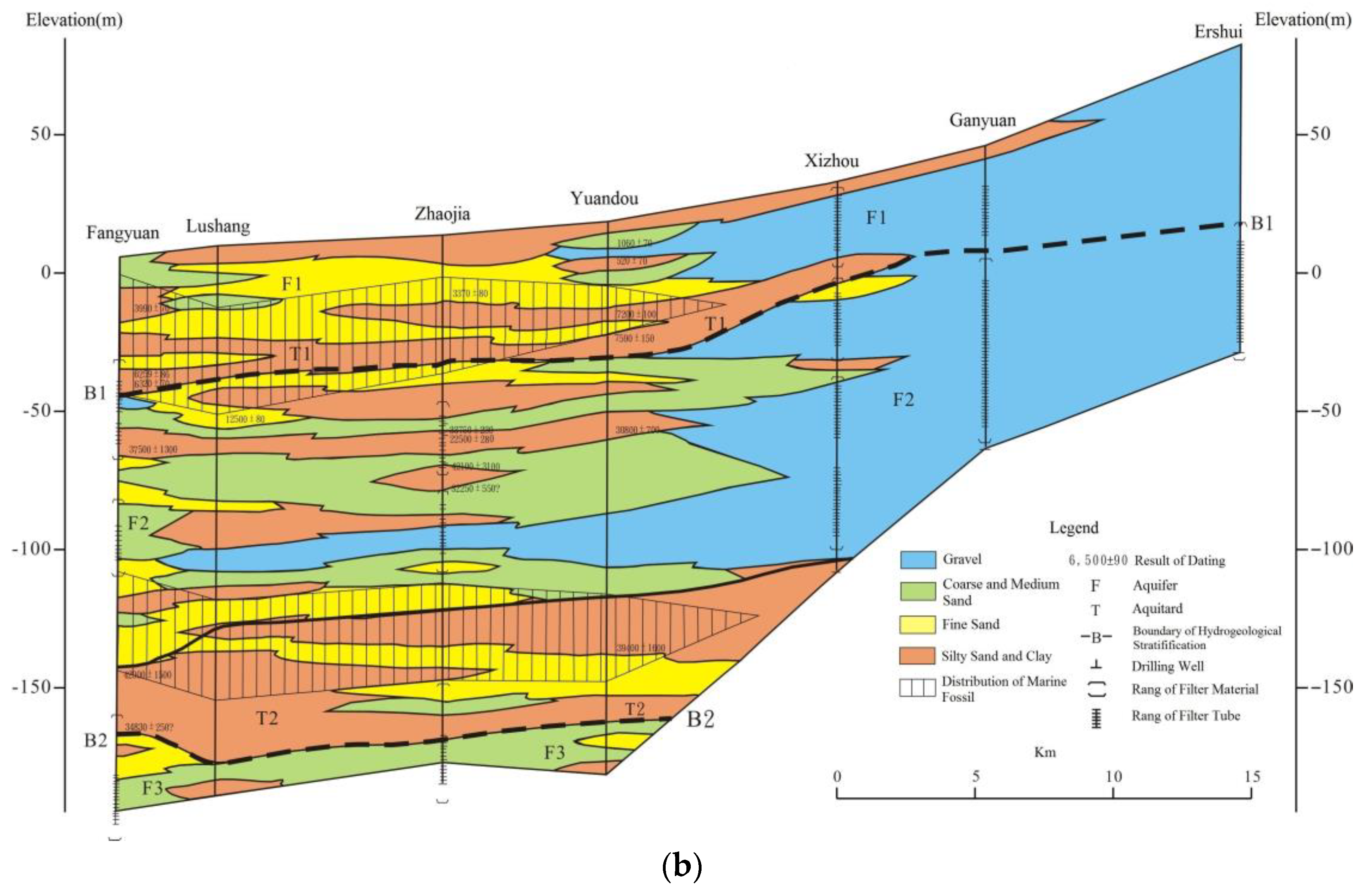
12]. According to the Chuoshui River Fan geology report published by Central Geology Survey [
13], the hydrogeological structures are: aquifer 1 (F1), aquitard 1 (T1), aquifer 2-1 and aquifer 2-2 (F2-1 and F2-2), aquitard 2 (T2), aquifer 3 (F3), aquitard 3 (T3), and aquifer 4 (F4) (
Figure 2b). The total thickness of the four aquifers is approximately 300 m.
According to the core and well logs, the Chuoshui River channel migrates to a new area every 2 to 3 decades, leaving old channels located in the area between the Old Chuoshui River and New Huwei River. Therefore, the sediments compositions are similar in the areas between the Old Chuoshui River and the New Huwei River [
13].
In this study area, the main water supply is from the groundwater resources. Although the amount of annual rainfall is high in summer, there is no reservoir to reserve surface water. Increases in population have increased the demand for water and consequently puts more stress on the groundwater system. The added stress increases subsidence and seawater intrusion.
3. Material and Method
3.1. Research Procedure
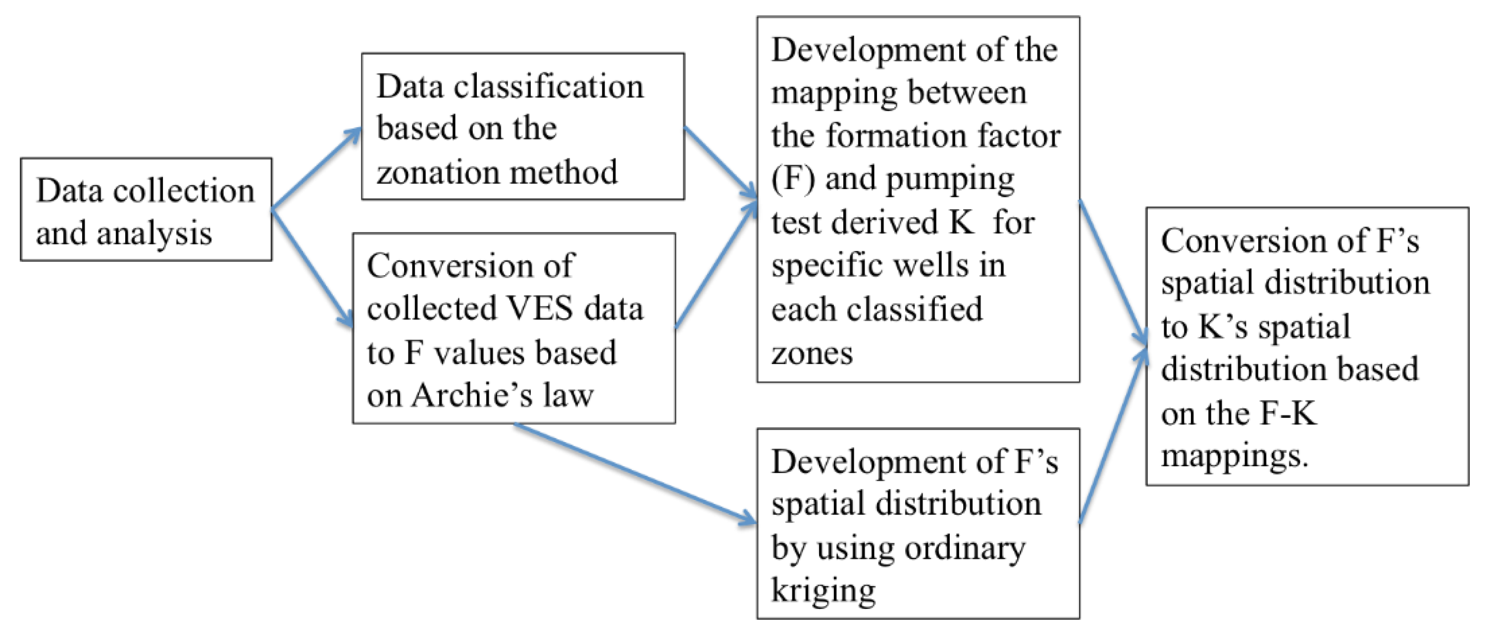
A general outline of the research procedure is presented in
Figure 3. In the figure, K, F*, and VES denote hydraulic conductivity, apparent formation factor, and vertical electrical sounding, respectively. In the first step, available data was collected from the Water Resources Agency and Central Geological Survey of Taiwan, including one-dimensional vertical electrical sounding (1D VES), pore water resistivity (
), core logs, and pumping test data(K). Next, the aquifers in the study area are classified into several zones based on the developed zonation method. The formation factor (F*) is then estimated by dividing the measured resistivity from VES surveys by the interpolated pore water resistivity from the observation wells. Next, we employed linear regression to establish the relationships between the estimated F* and pumping test derived K for each data group. Accordingly, all the F* values in the survey points can be converted into K values based on the K-F mappings. Finally, these K values are interpolated over the entire study area using the ordinary kriging method.
3.2. Data Collection and Analysis
The data utilized in the study contained 224 1-D VES measurements collected from Central Geology Survey (CGS) and 27 selected well data collected from the groundwater monitoring wells maintained by the Water Resource Agency (WRA). These well data included the core logs, pore water electrical conductivity, and the K derived by pumping tests. In addition, seven pore water electrical conductivity data were collected from the monitoring wells maintained by Taiwan’s Environmental Protection Administration. The original VES measurements had apparent resistivity and were inverted by IPI2WIN software (Version 3.0.1, Moscow State University, Moscow, Russia) [
14]. The water electrical conductivity (E
w) data collected from 34 (i.e., 27 + 7) wells were transferred into electrical resistivity (
) for the F value estimation.
3.3. Estimation of Apparent Formation Factor
The purpose of this study was to estimate the spatial distribution of K for the regional groundwater system based on the zonal K-F mappings. To achieve this purpose, the F* value of each aquifer at each VES survey point was estimated using Equation (4). The here represents the average resistivity value within a selected aquifer at the VES survey point. Additionally, since this study only considered estimating K for the saturated aquifers, only the VES data under the groundwater level was selected for the following analysis.
The amount of the values was less than that of the VES data, such that the values were interpolated over the study area with a 1 km by 1 km grid resolution based on the ordinary kriging method. Thus, the F values of the selected aquifers at the 224 VES survey points can be calculated by using Equation (4).
3.4. Data Classification-Zonation Method
Developing a symbolized K and F regression equation for the entire groundwater system was very difficult because there were many factors that affected the electrical resistivity measurements. According to previous studies [
15,
16,
17,
18,
19,
20], the sediment’s
*, m*,
w, S
w, and proportion of clay to a soil sample were the major factors that affected the electrical resistivity measurements. Because this study only considers the saturated aquifer, S
w is not considered as a classification factor in the zonation method. Based on these factors, a zonation method was proposed to discrete the groundwater system into several zones to reach the condition that the sediment composition inside a zone was similar, which resulted in a similar electrical resistivity characteristic.
The zonation method considers three physical factors: area of fan delta, aquifer layer, and aquifer type. In general, the sediments of a fan delta may have its own sediment composition, since each fan delta consists of its own river network that transports sediments originated from the mountains with their specific geological formations. Accordingly, the electrical property, such as m*, , and α*, of the sediments may vary with fan delta, and the rivers in the boundary of fan deltas will be used to access the area of a fan delta.
For the aquifer layers, in general, the sediments of the deeper aquifers are older than those of a shallow aquifer (e.g., drilling downward will yield newer material first followed by subsequently older material). Older sediments become compressed with age, causing them to have lower and m* than younger sediments. Here, we adopt the aquifer layers determined by Taiwan’s CGS to conduct zonation analysis.
For the aquifer type, it affects the measured electrical resistivity as well. The sediments of the unconfined aquifer have less clay than that of the confined aquifer. A large number of publications [
15,
16,
17,
18,
19,
20] indicate that the electrical properties of clay are quite different from that of gravel and sand because clay has excess electrical conductivity due to its electrical double layer.
To determine the boundary of unconfined and confined aquifers between the fan top and middle fan areas, the collected core logs were manually classified into two types: confined and unconfined types, depending on whether there was clayey matter on the top of the core logs or not. Next, the classified core logs and their associated F* values were analyzed by the decision tree with pruned three using XLminer version 2018 to determine the F* value as the criteria to identify the boundary of the unconfined aquifer.
According to these three factors, a groundwater system can be divided into several zones, and the K and F* data pairs can be classified into groups based on the identified zones.
3.5. Mappings between Hydraulic Conductivity and Formation Factor and Hydraulic Conductivity Fields Estimation
To develop the K-F* mappings, the K-F* data pair were carefully selected. In general, saturated coarse grain has high resistivity, while saturated fine grain has relative low resistivity. An F* value at a VES survey point was selected to develop the K-F* mapping only when the vertical resistivity distribution at this survey point was consistent to the vertical sediment distribution of its neighbor wellbore log. Once they were consistent, the F* and the K from the neighbor well were selected as a data pair to develop the K-F* mapping.
This study applies linear regression to develop the relationship between K and F* for each classified zone. According to previous studies [
7,
10], linear regression has already been used to successfully develop the relationship between K and F*, because the relationship between K and F* is almost linear (e.g., Equation (7) in the results and discussions section).
After the K-F* mapping of each zone was developed, these mappings were used to convert the F* values at the VES survey points into the K values. We then employed the ordinary kiging method to interpolate these K values over the entire study area. Further details are shown in the next section.
4. Results and Discussions
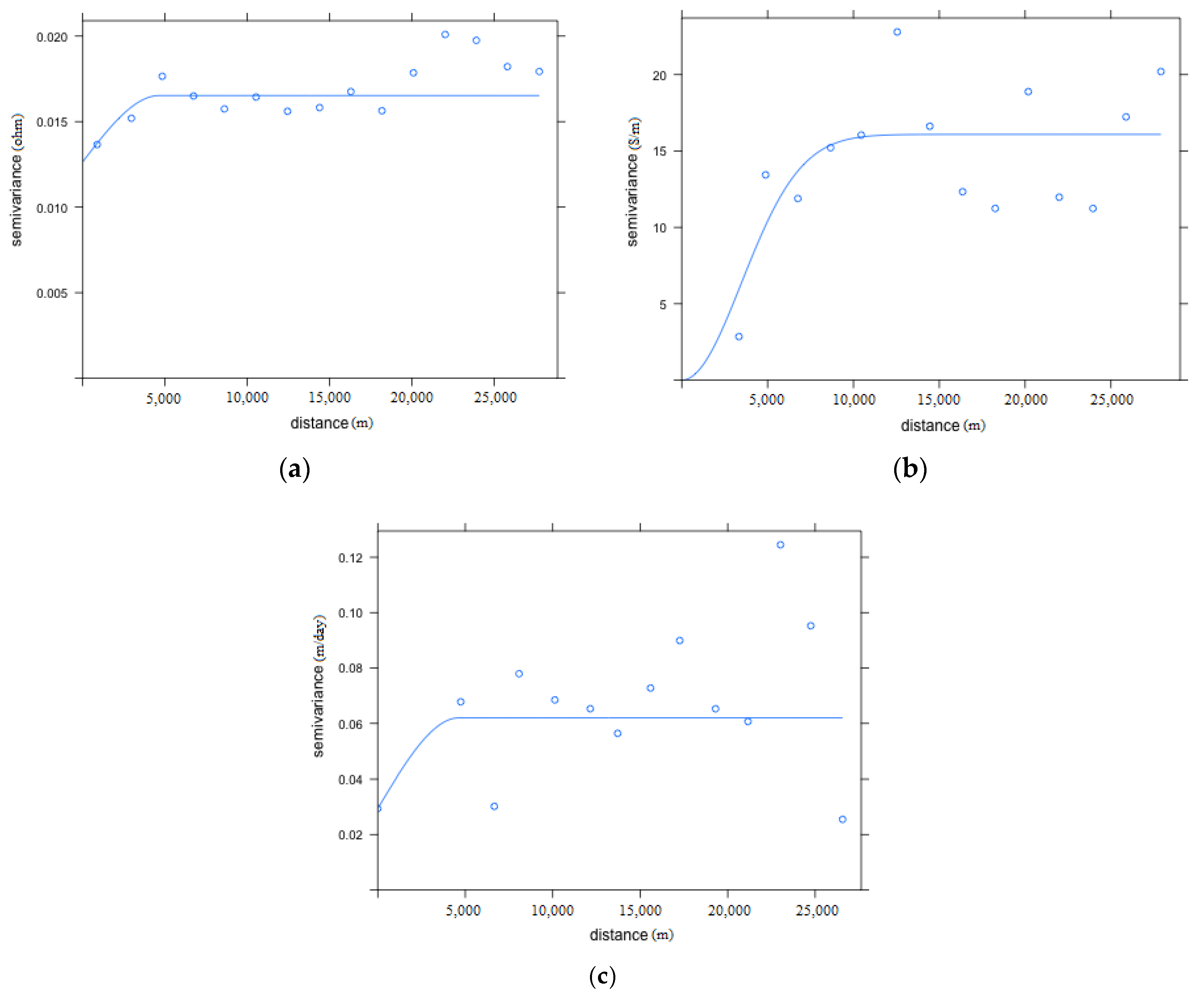
4.1. Estimation of the Correlation Scale for the Collected Data
The ordinary kiging method was important in this research procedure, since this method was used to interpolate the collected point data over the entire study area. To conduct the ordinary kiging method, the geostatistic analysis for the collected data (i.e.,
,
, and K) was conducted by Rockworks 16 (
www.RockWare.com). The Gaussian model, shown in Equation (5), was used to fit the experimental variogram in both major and minor axes, resulting in an anisotropic variogram model:
where
is the variogram, h is the distance between two locations, and a is the parameter of the Gaussian model. To improve the results of variogram model fitting, except
, the collected data were normalized based on Equation (6), where
denotes the scaled value of data
, and
and
denote the minimum and maximum values of the collected data set, respectively. The normalized values were also used to conduct kriging interpolation, and the interpolated values were converted into real values by using Equation (7):
The parameters of the experimental variograms for the three types of collected data are shown in
Table 1. The calculated correlation scale values of the three types of data were very close. The varigram-fit diagrams are shown in
Figure 4, which shows that the semivariance of VES was relative stable compared to that of
and K. This was because the amount of the VES data was dense in the study area, and was about five times higher than that of the well data. According to
Table 1, the correlation scale values (i.e., range) of VES,
, and K were 4643, 4900, and 4935, respectively. These geostastic parameters were then used for the following kiging interpolations.
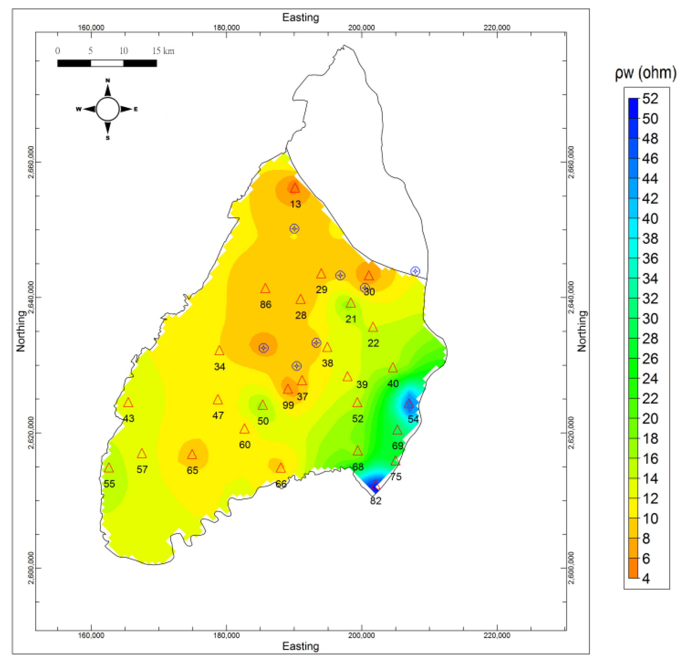
4.2. Apparent Formation Factor Estimation
In order to estimate the F* values at all the VES survey points, the pore water resistivity values sampled from the observation wells were interpolated over the entire study area (
Figure 5).
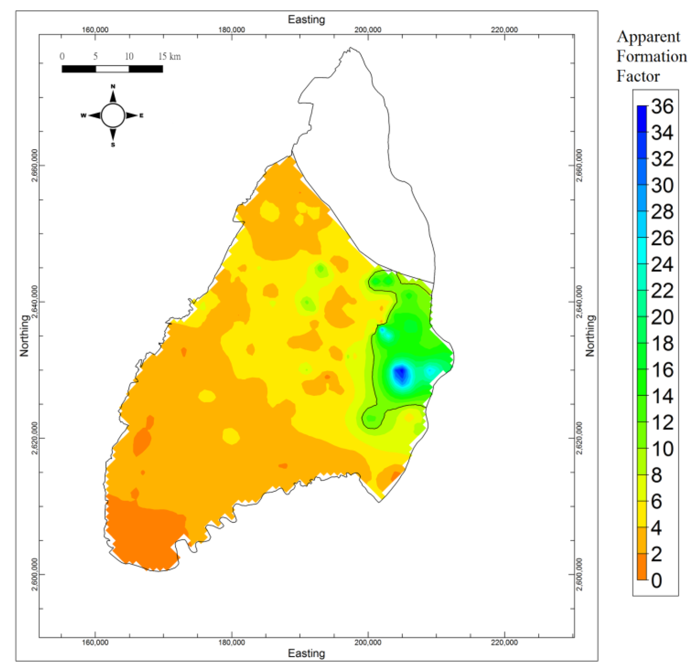
Figure 6 shows the spatial distribution of the estimated F* of the shallow aquifer. The F* values in the most non-fan-top areas were less than five, while these values in the fan-top areas were greater than 10.
Notice that the F* values could not be calculated for the entire study area, because the amount of data for the observation well in the Wu river area was little (only four points), which resulted in an unreasonable spatial distribution of kriged . In addition, this study only analyzed the aquifers 1 and 2-1, since the resolution of VES data is poor over the depth of 100 m. In the Beguan River fan delta, the sediments were muddy, which resulted in the limitation of exploration depth (i.e., the average exploration depth is 50 m). Thus, in the Beguan River fan delta, only the VES data within the shallow aquifer could be used to estimate the K field.
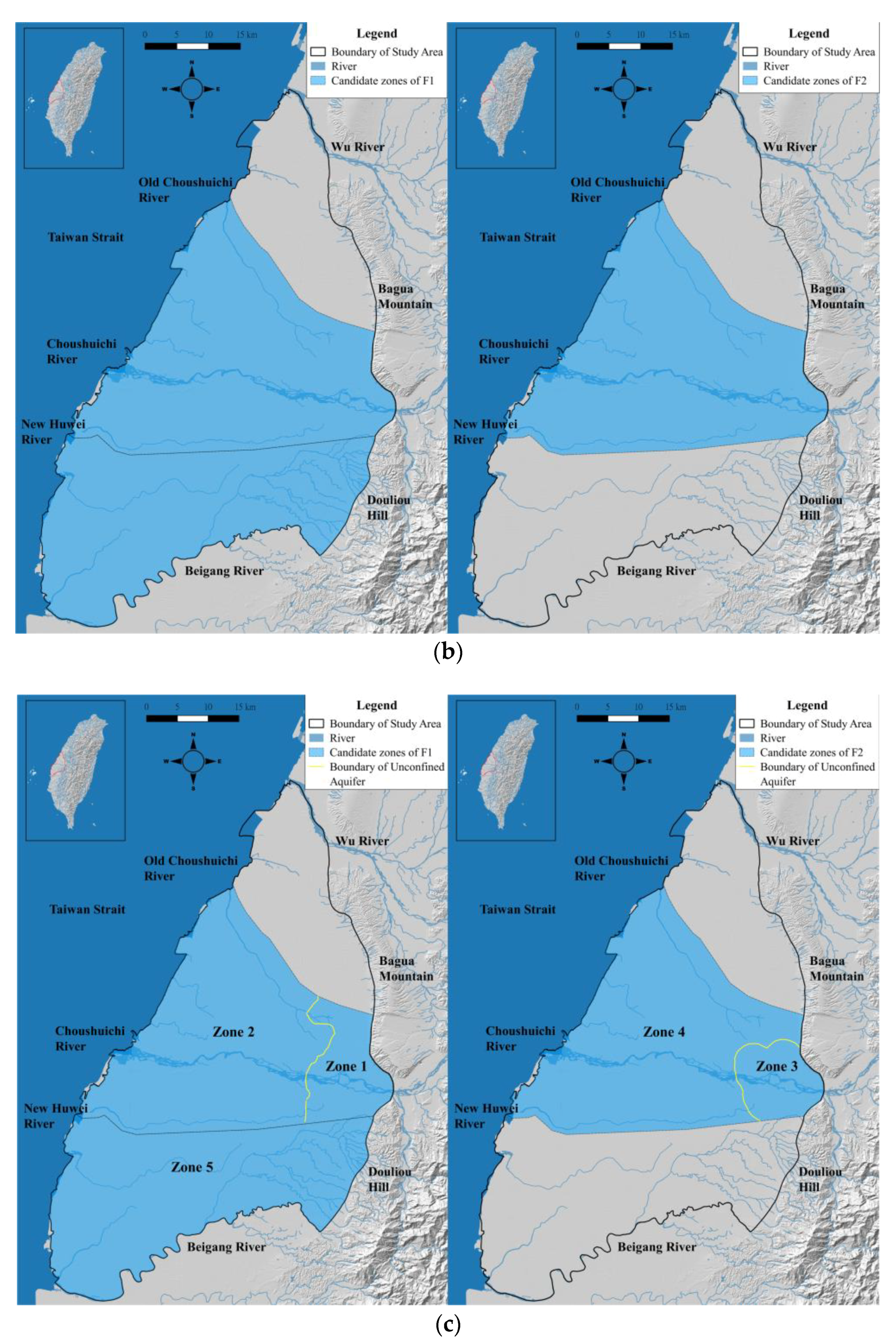
4.3. Data Classification Analysis
According to the proposed zonation method, the study area was divided into multiple zones. The original stratigraphy of the study area is presented in
Figure 7a; only aquifers 1 (F1) and 2-1 (F2-1) were considered in this study, due to the limitation of data resolution of VES. Using the three fan deltas in the study area, the Wu river, Beigun river, and Chuoshui River fan deltas, the aquifer was refined into six zones. However, because of the data limitation shown in
Section 4.2, the Wu River fan delta and the second aquifer of Beigun river fan delta were eliminated.
CGS collected 88 core samples from the wells, shown in
Figure 7a, for C-14 dating in the study area. According to the C-14 dating records, the deposition chronology of F1 was less than 10,000 years; that of F2-1 was in the range between 20,000 and 30,000. Therefore, F1 and F2-1 of the Chuoshui River fan delta (i.e., the area between the Old Chuoshui River and the New Huwei River) were divided into two different zones. The selected candidate areas are shown in
Figure 7b.
The shallow aquifer of Beguin River fan delta is a confined aquifer, and the aquifers of Chuoshui River fan delta can be further divided into confined and unconfined aquifers. Based on the analysis results of the decision tree, an F* value of around 10 was used as the criteria to access the boundary of the unconfined aquifer. Accordingly, we set the contour line of F* = 10 to distinguish the aquifers into unconfined and confined aquifers for the Chuoshui River fan delta (
Figure 6).
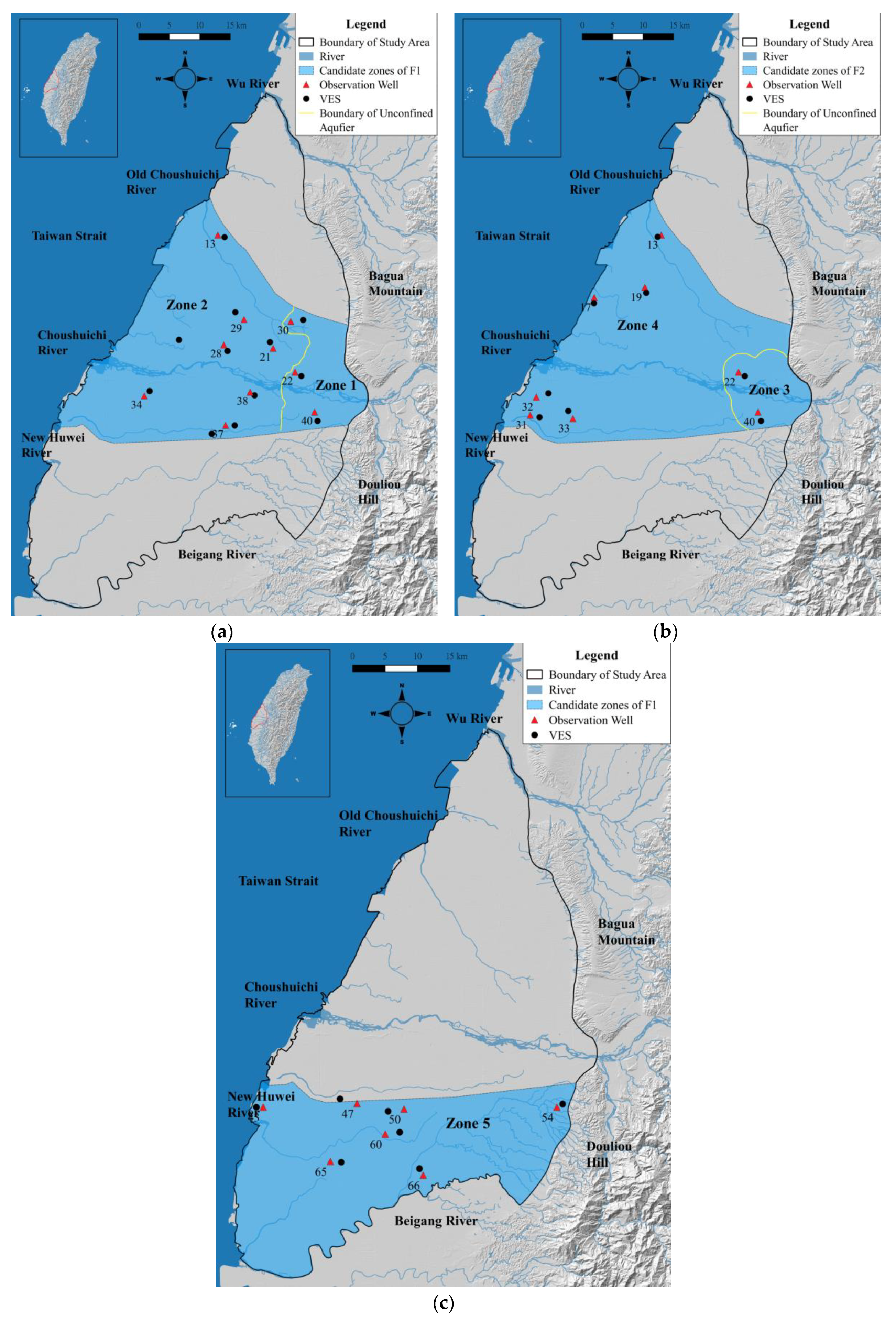
As a result of the data classification, the study area was classified into five zones, which are shown in
Figure 7c. The data pairs were classified into five groups based on the five zones, as shown in
Table 2.
Figure 8a–c show the five zones and the locations of the selected wells and VES survey points. Due to the limited data within zone 3 (i.e., only two data pairs), this zone was eliminated from the candidate zones. Finally, the selected four zones for data pair classification are zone 1, zone 2, zone 4, and zone 5. The selected K-F* data pairs are shown in
Table 2.
The correlation coefficients between the F* and K data pairs improved after the zonation method was applied for the selected data pairs. The cross correlation of the original data set was 0.61. After the zonation method was applied to the data pairs, the cross correlations of zones 1, 2, 4, and 5 improved to 0.81, 0.85, 0.87, and 0.91, respectively.
4.4. Mappings between Hydraulic Conductivity and Formation Factor
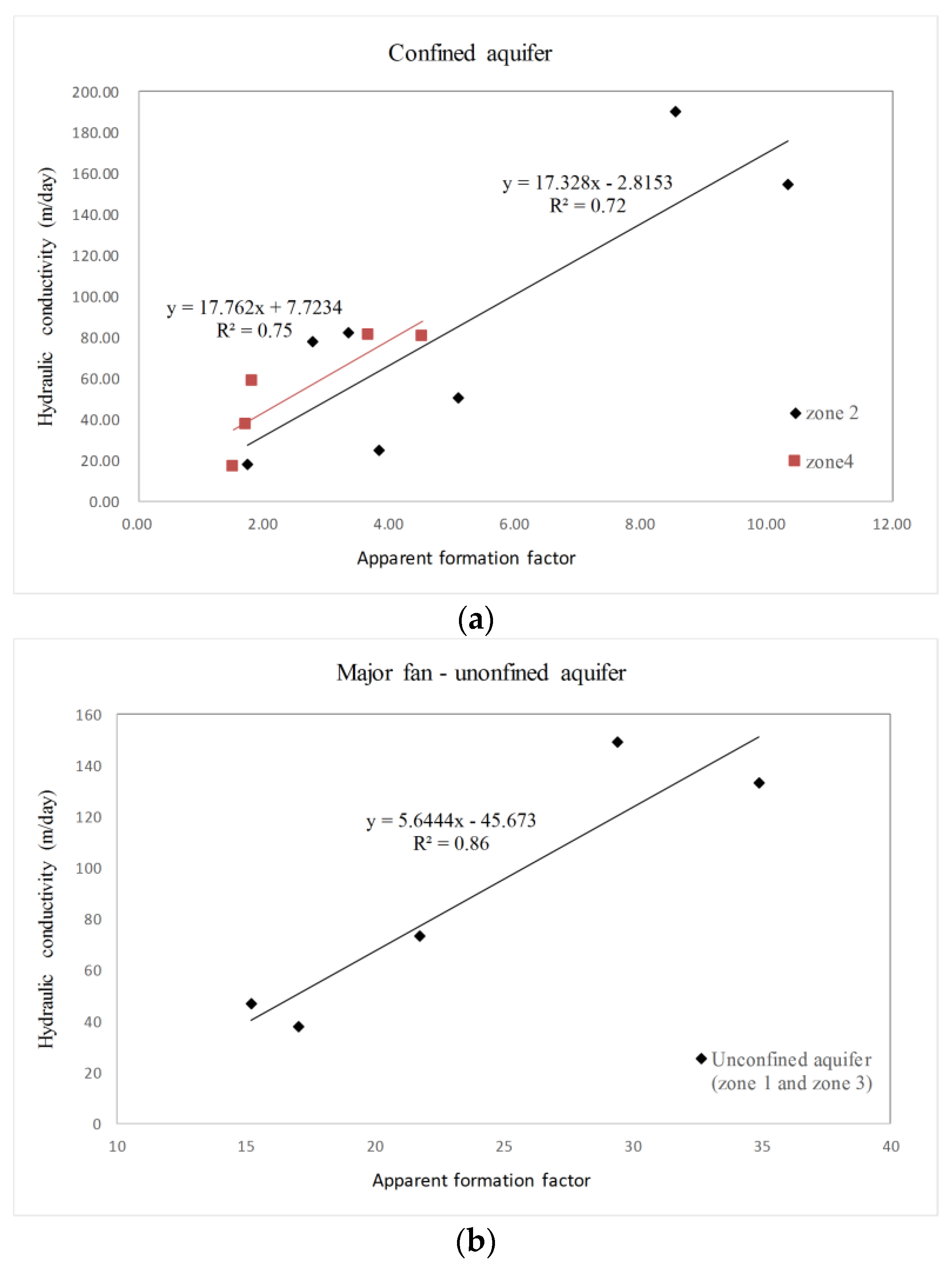
Linear regression of K-F* data pairs from selected zones provided the framework to develop a set of K-F* mappings. The regression results are presented in
Figure 9, and Equations (8)–(11). In
Figure 9a, the red and black solid circles denote the data pairs of zone 2 and zone 4, respectively. The regression results for R
2 values of the two regression equations (i.e., Equations (8) and (9)) were 0.72 and 0.75, respectively. In addition, the two regression equations showed that their slopes are very close. This reveals that ‘deposition chronology’ was insensitive to the K-F* mappings, and might not be necessary to be considered as a classification factor. This result might have been caused by the insignificant variance of the sediment composition: less than the VES exploration depth of 100 m in this study.
Figure 9b shows the regression result of zone 1 and zone 3. Since the deposition chronology was not necessary to be considered in the data classification, the K-F* data pairs in unconfined aquifer areas, zone 1 and zone 3, were integrated to develop K-F* mapping for the unconfined aquifer. The regression equation of unconfined aquifer is shown in Equation (10), with an R
2 value of 0.87.
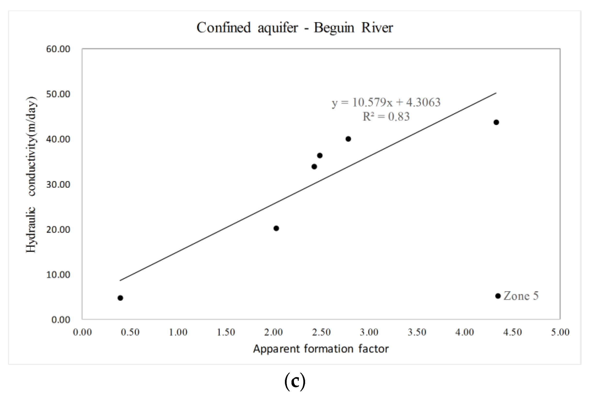
Figure 9c shows the regression result of zone 5. The regression equation of zone 5 is presented in Equation (11) with an R
2 value of 0.84. By comparing the slopes of Equations (8) and (11), the difference between the two values (i.e., 10.58 and 17.33) is obvious, which resulted from different sediment composition between the two zones (i.e., zone 2 and zone 5 are located in different fan deltas). The sediment composition of the Begun river area (zone 5) consists of more muddy matters than that of the major fan areas (zone 1 to zone 4). Therefore, considering fan delta as a classification factor was necessary for better regression results.
4.5. Spatial Distribution of Hydraulic Conductivity
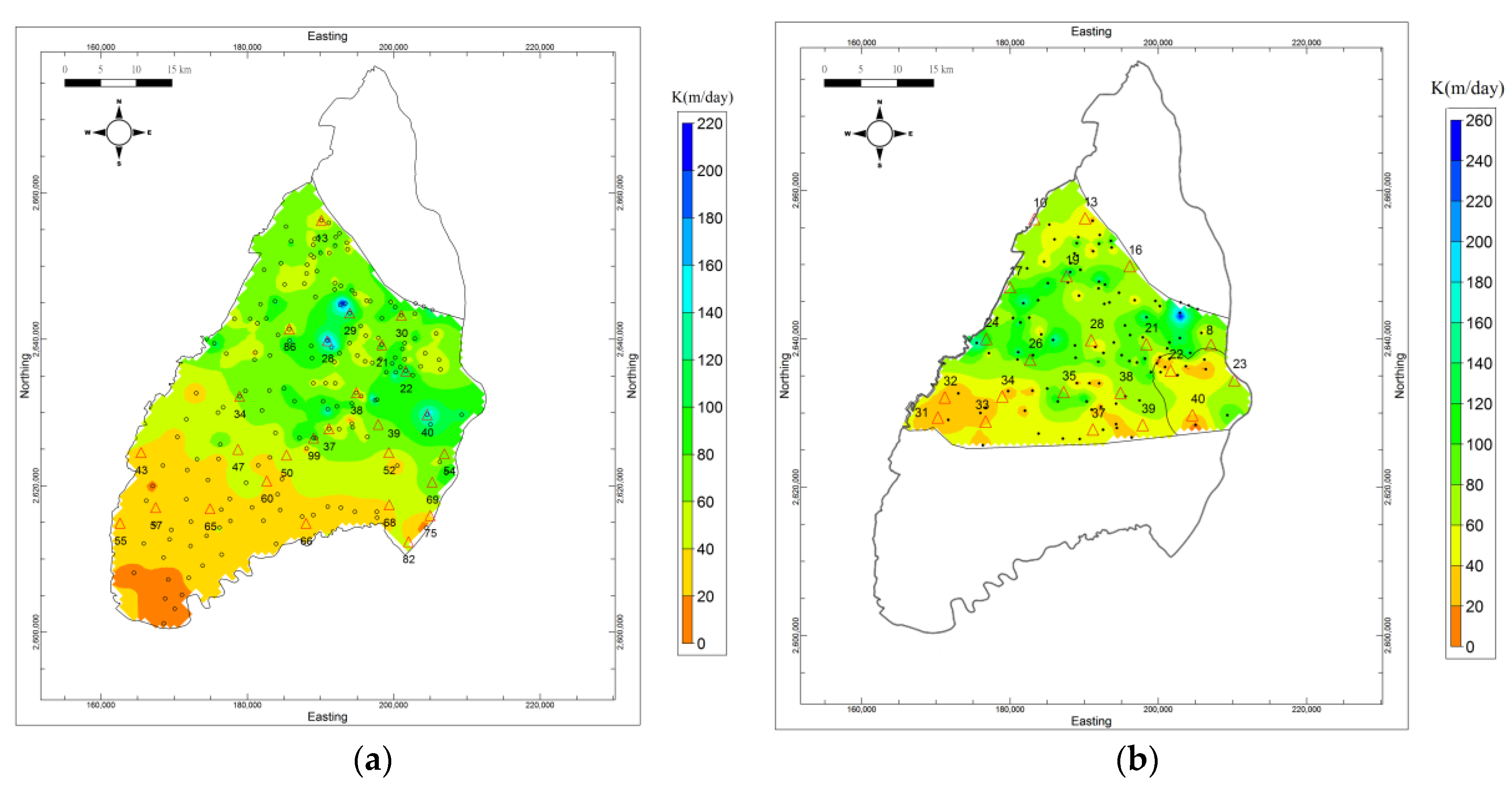
The estimated spatial distribution of K for zone 1 to zone 5 is shown in
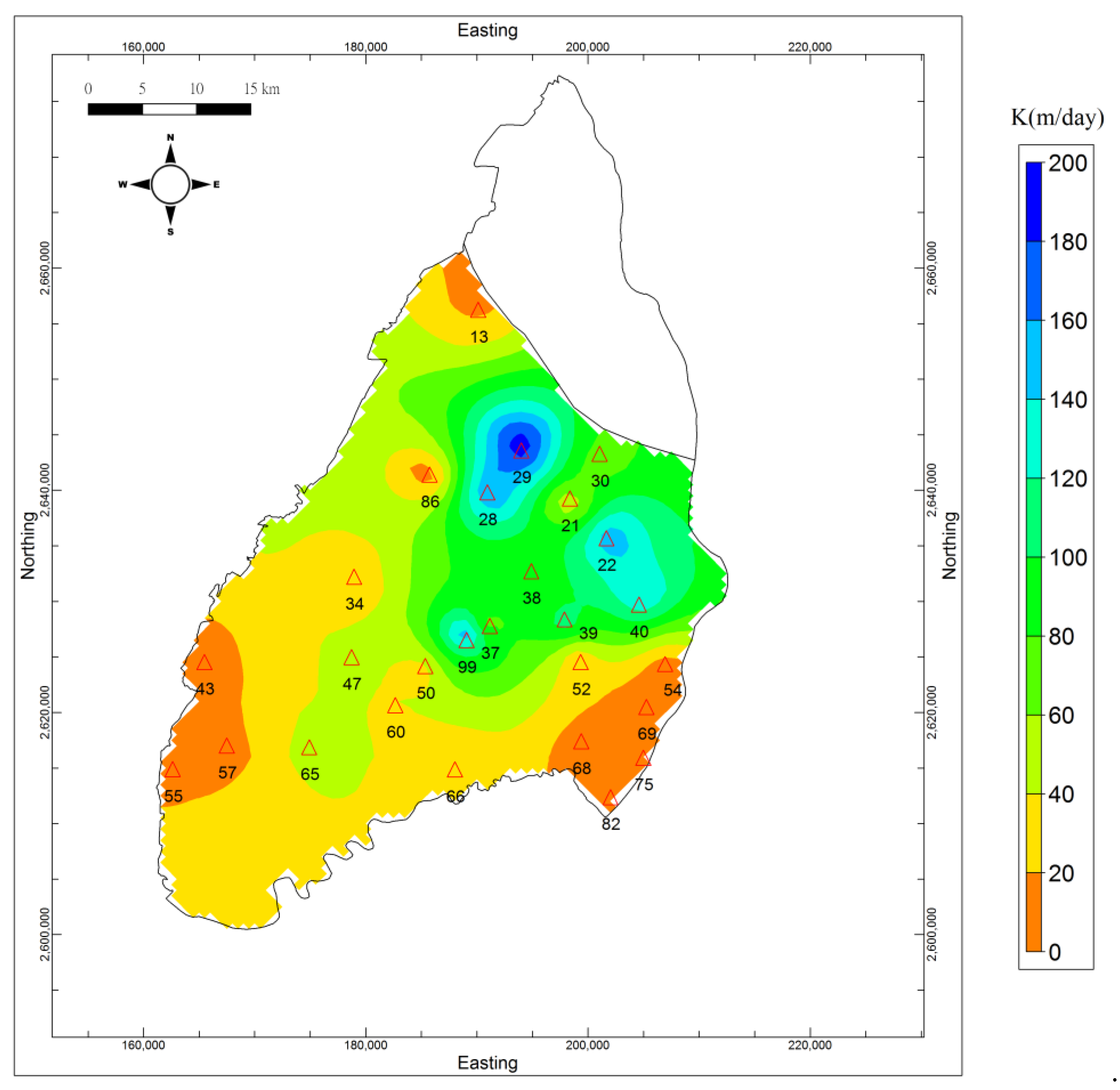
Figure 10.
Figure 10a shows that most of zone 1’s K values were greater than 60 m/day, while the maximum K value approximated at 160 m/day. Within zone 2, the K values in the areas between wells 13 and 34 ranged from 20 to 120 m/day, the K values between wells 30 and 38 ranged from 20 to 80 m/day, and the K values between wells 28 and 29 ranged from 100 to 200 m/day. The spatial variation of K values in zone 5 was much less than that of the zone 1 and zone 2. The majority of zone 5’s K values were in the range of 20–40 m/day, and parts of the K values in the south area were even less than 20 m/day, which reveals the features of the hydraulic property of clayey sediments.
Figure 10b shows the spatial K for zone 3 and zone 4. The K values were relative low in the zone 3 area, while the K values were relative high in the zone 4 area. We supposed that the unconfined aquifer in the zone 3 would have high K values. However, the results were not consistent with our expectation. The reason why zone 3 had relative low K values was because the selected observation wells were close to the boundary of zone 3, and the interpolation of the
values from these wells were relative high, resulting in relatively low F* values, accompanied with relative low K values. Thus, the kriged K values in the zone 3 were dominated by these low K points, and represented a relative low-K area compared to zone 4. In addition to the low K values, we noticed that the VES survey points in zone 3 were not as dense as those in zone 4, and the estimated K field of zone 3 might have changed if we had increased the
measurements and VES survey points in the center area of zone 3.
4.6. Validation of the Estimated K Values with Field Test Data
The verification results show that the estimated K values were reasonable. This study used the data collected from the addition of nine pumping tests, which was conducted by the WRA, to verify the estimated results. The wells used for validation are listed in
Table 3, and their locations are shown in
Figure 1 with a green triangle.
Table 3 presents the verification of the K values estimated by the proposed method. The absolute difference between the measured and estimated K were in the range between 3.8 and 58.3 m/day, and the correlation coefficient between the two data sets reached 0.93. Most of the estimated K values fit the observed K values. Although the absolute difference of well 99 (58.3 m/day) was slightly high in the verification, the estimated results were within one order of magnitude. Schwartz and Zhang [
21] indicated that the K variation of each lithology can be three orders of magnitude. Therefore, the estimated results remain acceptable. Importantly, in addition to the direct comparison of the measured and estimated K, the high correlation coefficient of the two data sets (i.e., 0.93) indicated that the proposed method can catch the spatial trend/variation of the real K fields for a regional groundwater basin.
4.7. Comparison between the K Fields Estimated by the Developed Method and the Ordinary Kriging Method
The estimated experimental variograms between the original pumping test K values and our estimated K values were similar. The major and minor ranges of the two data sets were close (shown in
Table 1), and these results show that the amount and spatial distribution of groundwater wells were able to delineate K’s spatial correlation for the study area. Although the correlation scales of the two data sets were very close, the amount and spatial distribution of the two data sets were quite different resulting in different kriged spatial K with different resolution.
The spatial distribution of K, estimated by the proposed method, integrated both well data and VES measurements and was able to represent K variation with a much higher resolution than the one derived from kriging pumping test K values.
Figure 10a and
Figure 11 show the spatial K of the shallow aquifer estimated by the developed method and the kriging method, respectively.
Figure 10a shows that K varies significantly from the fan-top to the middle-fan areas, while
Figure 11 shows that K varies relatively smoothly everywhere in the study area. For example, in the areas between wells 28 and 38, the K values of
Figure 10a ranged from 20 to 200 m/day, with a relatively sharp spatial variation, while K values in
Figure 11 ranged from 100 to 140 m/day with a smoothly spatial variation. Moreover, the high K zones of
Figure 11 include zone 1, zone 2, and part of zone 5, while in
Figure 10a, high K zones only existed in zone 1. These two examples show that the proposed method can delineate more detailed features of the K fields in both local and regional scales than the ordinary kriging method can.
The study results reveal that the developed method is an efficient and economical method to increase the amount of K for a regional groundwater system. A pumping test was necessary for collecting K, which was the solid data. However, relying on pumping tests results in limited estimates of K, due to it being time consuming and it having high well installation costs. By properly integrating the VES and well data, the developed method can delineate the relative detailed features of K fields for regional aquifers. This results in a faster, less expensive improvement on K estimates as compared to constructing additional wells and conducting pumping tests.
5. Conclusions
This study developed a method to estimate the spatial distribution of K for a composite fan delta by integrating dense VES measurements with some pumping test data. The key component of this advanced approach is the developed data classification method, which was conducted using a physical-based zonation method and was used to divide the data pairs into several groups. The results showed good agreement between the regression models and the observed data pairs, and the correlation coefficient of each grouped K-F data pairs reached 0.8+. With this small estimation error and a high correlation coefficient, this zonation method was practicable for our data classification. Additionally, the deposition chronology was insensitive to the K-F mapping. Thus, only two factors, fan delta and aquifer type, need to be considered in the developed zonation method.
By integrating highly dense electrical resistivity measurements and some pumping test data, the developed approach makes spatial K estimation for a regional groundwater system more efficient and economical than only relying on traditional pumping tests. Moreover, the local and regional features of K in a composite fan delta can be clearly delineated. This will lead to an accurate flow field prediction in various scales, and thus, the accuracy of the groundwater analyses will be significantly improved.


