Abstract
Steps effectively dissipate the energy of water along a path and reduce the size of the stilling basin but are rarely used in curved spillways. The shore spillway of a reservoir, which is restricted by topography, must be arranged in a curved shape. At high flow velocity and low water depth, some areas of the base plate of the curved spillway were not covered by the water. The water flow into the stilling basin did not form a submerged hydraulic jump. It was proposed that a step with bottom non-uniform heights be placed in the smooth base plate of the curved spillway to improve these undesirable hydraulic phenomena. A physical model experiment with a length scale of 1:40 verified the feasibility of the curved stepped spillway in engineering. Based on the k-ε model and volume-of-fluid (VOF) method, a three-dimensional numerical model was established, and the reliability of the numerical model was verified by measured data. The main flow region, velocity field, cavitation on a step, and the energy loss rate of steps were discussed. The comparison between a curved spillway with and without steps shows that the steps balance the partial centrifugal force in the curved section, making the water depth of the cross-section evenly distributed, and the base plate was no longer covered by water. The flow pattern on the steps was skimming flow, and the velocity of the flow into the stilling basin was greatly reduced. The elevation of the concave bank of the base plate was raised, resulting in the formation of transverse flow, which in turn constituted a three-dimensional energy dissipation pattern with the longitudinal flow. The energy loss was significantly higher than that of the smooth curved spillway. However, the triangular region near to the concave bank on the base plate experienced negative pressure, and an aeration device in front of the steps was needed.
1. Introduction
Spillways are a major part of hydraulic engineering for the prevention or control of floods. A reservoir’s shore spillway is located in mountainous terrain. Due to the restriction of its topography and geology, the spillway must be arranged in a curved shape with a slope of 1:3.5. The flow in this spillway is affected by centrifugal force, resulting in secondary flow, as well as an apparent difference in the water level between the concave bank and convex bank [1]. Additionally, there are parts of the base plate in the bend that are not covered by the water. Furthermore, the velocity of the water flow into the stilling basin is large and the flow state is poor. The steps with non-uniform heights at the bottom were placed in the curved spillway to improve these undesirable hydraulic phenomena.
Although there are few practical engineering and research achievements in the inclusion of steps in curved conduit flow, a considerable number of published works have been devoted to the straight stepped spillway, which can provide a reliable reference for this study. A stepped spillway can effectively dissipate energy and thus reduce the size of the stilling basin in the downstream area [2,3]. A hydraulic model experiment by Sorensen [4] suggested that the stepped spillway has a good energy dissipation effect and that the flow from the crest to the part of the step can easily and smoothly transition. Additionally, Shvainshtein [5] conducted a series of hydraulic model tests to estimate the total energy loss from a stepped spillway and found that the energy dissipation rate was maximum in a nappe flow regime and that the dissipation rate can reach 75% of the total in a skimming flow regime. Furthermore, Christodoulou showed that in the skimming flow condition, the energy loss was primarily dependent upon the ratio of the critical depth of flow passing over the spillway to the step height, as well as on the steps’ number [6]. Moreover, Felder et al. studied a moderate slope stepped spillway with non-uniform step heights (26.6°); five stepped configurations in were tested, where is the critical water depth measured by the step edges and is the vertical step height. The results indicated that the energy dissipation rate of uniform and non-uniform step height was basically the same [7]. Further studies of air entrainment and pressure and velocity fields were conducted by Pegram et al. [8], Ostad et al. [9], Meireles et al. [10], and Zhang G et al. [11].
Numerical models are a good supplement to capture the characteristics of intricate flow, and significantly decrease costs compared with physical experiments. Such models have been applied to simulate the flow characteristics of a stepped spillway. For example, Chen et al. [12] presented a three-dimensional (3D) calculation method for applications to the irregular boundaries of the stepped spillway and to simulate the complex turbulence overflow. An unstructured grid was applied to fit the boundaries and the overflow was simulated by the 3D k-ε turbulence model. Ye et al. [13] adopted the volume-of-fluid (VOF) method to track the water surface, and the k-ε model to simulate the 3D turbulent flow of an s-shaped stepped spillway. Tabbara et al. [14] also used the 3D k-ε turbulence model to predict the main performance of the flow and found that the predicted water surface profile and energy dissipation were in close agreement with experimental results. The hydraulic characteristics of stepped spillways have also been simulated by other turbulence models. For instance, Toro et al. [15,16] numerically modeled the non-aerated skimming flow over a stepped spillway using the Detached Eddy Simulation (DES) model, and paid more attention to the 3D instantaneous velocity and vorticity fields on the step cavities.
The purpose of this study was to experimentally and numerically analyze the energy dissipation effect of non-uniform-height steps applied in a curved spillway, and to analyze the effect of ensuring that the base plate is completely covered by water. The feasibility of the curved spillway with non-uniform-height steps in engineering and the accuracy of the numerical model were verified by a physical model experiment. More comprehensive hydraulic characteristics, such as the velocity distribution in cross-section, the shape of the free surface, and the pressure distribution along the path, were investigated through numerical simulation.
The experimental model and the non-uniform-height steps are introduced in the next section (Section 2), followed by the numerical methodology (Section 3). In the numerical methodology section, the reliability of the numerical model is verified by comparison with measured data. In the results section (Section 4), the main flow region is presented and the 3D flow structure on the steps is analyzed by velocity fields in different coordinate axes. The position where cavitation may occur is indicated according to the pressure on the wall and the base plate of the step. The energy dissipation rate is also given in the results section.
2. Physical Model and Problem Description
2.1. Physical Model
The shore spillway was of a curved type due to topographic restrictions, as shown in Figure 1a. The curved spillway of the prototype was composed of a control section, a constriction section, a curved section, a chute rear section, and a stilling pool. The total length of the spillway was 212.74 m, excluding the stilling basin, and the slope was 1:3.5. In the constriction section, the width of the base plate narrowed from 14 to 10 m, with the constriction angle being 1.35°. The radius of the curved section was 150 m after projection to the horizontal plane, and the angle of curvature was 33.85°. The width of the chute rear section was 10 m. The maximum discharge flow was 448 m3/s, the maximum flow of the unit width was 44.8 m3/s, and the maximum head was 518.36 m.
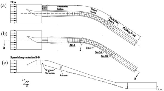
Figure 1.
Diagram of a reservoir spillway. (a) Top view of smooth spillway; (b) top view of stepped spillway; (c) side view of stepped spillway. “A” denotes step No. 9.
For the curved spillway with non-uniform step height, 28 steps were placed in the base plate, as shown in Figure 1b,c. The origin of the Cartesian coordinate system was located at the weir crest, and the x, y, and z axes were aligned in the cross-section direction, along the path, and in the water depth direction, respectively. The design of the non-uniform-height steps, shown in Figure 2, meets the following two requirements:
where and are the bottom elevations of the concave bank steps, and and are the bottom elevations of the convex bank steps.
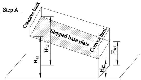
Figure 2.
Schematic of step No. 9 with non-uniform heights at the bottom.
The physical model was constructed to a length scale of 1:40; the overall arrangement is shown in Figure 3. The experimental conditions for both spillways are shown in Table 1. The spillway of the prototype was made of concrete and had a roughness of 0.014, so the corresponding model roughness was 0.0076. To meet the roughness requirement, the physical model was made of plexiglass.
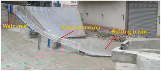
Figure 3.
The experimental arrangement of the reservoir.

Table 1.
The conditions of the prototype and physical experimental model.
The physical model experiments were conducted at the State Key Laboratory of Hydraulics and Mountain River Engineering, Chengdu, China. The results of the physical model at a discharge rate of 272.0 m3/s of the prototype is presented in this study. The velocity was measured using a propeller-type current meter and pitot tube, and the time-averaged pressure was measured using a piezometer tube. The accuracy of the gauge used for measuring water depth was ± 1 mm. The flow visualizations were conducted with a digital video camera (Canon D800).
2.2. Problem Description
As a result of the inertial centrifugal force, the water surface elevation on the concave bank was higher than that of the convex bank in bends of the curved spillway, as shown in Figure 4. stands for the water level of the convex bank. The difference in water level between the concave bank and convex bank, , can be calculated by the Rozovskiĭ equation (seen in Equation (1)) [17].
where is the transverse gradient of the water surface at some point; and denote the gravity acceleration and von Karman constant, respectively; C represents the Chezy coefficient; is the mean velocity in the vertical direction; and R is the radius of curve curvature.
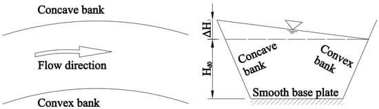
Figure 4.
Water levels on the concave bank and convex bank.
In Equation (1), when the radius R is constant, the transverse gradient will increase with the increase of velocity . If the velocity is large enough, will also become larger, and even extreme hydraulic phenomena will occur for the conditions in Table 1. This phenomenon is that the water level () on the concave bank will be extremely high, while there is no water on the base plate near the convex bank, as shown in Figure 5a. This phenomenon was also observed in the engineering experiment of Wu et al. [18]. Additionally, the adverse water flows from the curved section into the stilling basin, resulting in a lower water depth and unformed submerged hydraulic jump in the stilling basin, as shown in Figure 5b.
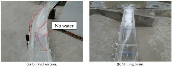
Figure 5.
Flow regime in the curved section and stilling basin of the smooth spillway.
2.3. Effects of the Non-Uniform Steps
To improve these undesirable hydraulic phenomena, the steps with non-uniform height at the bottom were placed on the curved spillway. The flow pattern of the curved spillway was greatly improved, as shown in Figure 6. The difference in water level between the concave bank and the convex bank, , decreased in the curved section, and the base plate near the convex bank was covered with water, as shown in Figure 7a. The stable submerged hydraulic jump which formed in the stilling basin was able to effectively dissipate energy, as shown in Figure 7b.
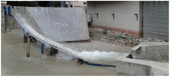
Figure 6.
Flow pattern of the curved stepped spillway.
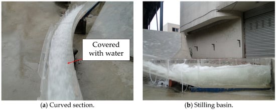
Figure 7.
Flow regime in the curved section and stilling basin of the stepped spillway.
The average water depths at different measuring points on the concave bank and convex bank of the curved section at a flow discharge rate of 272.0 m3/s of the prototype are given in Table 2. For the concave bank of the smooth spillway, the water level was obviously higher than that of the convex bank, and the water level was extremely low (0.08 m) at an axial distance of 161.35 m, which was close to the bad flow state without water covering the base plate. The non-uniform-height steps proposed in this study were placed in the smooth spillway, which caused the difference in the transverse water level on the cross-section to decrease obviously. The flow velocity distribution was more uniform, which significantly improved the flow regime in the curved section. The cross-section velocity distribution of the curved stepped spillway is given in Table 3.
Table 2.
The average water depths of each measuring point at a flow discharge rate of 272.0 m3/s of the prototype.
Table 3.
The cross-sectional velocity distribution of the curved stepped spillway at a flow discharge rate of 272.0 m3/s of the prototype.
3. Numerical Methodology and Model Validation
It is difficult to capture detailed information about complex flow using the physical model experiment. To understand the hydraulic characteristics of the curved spillway more intuitively and comprehensively, the numerical model was used to conduct further study. The reliability of the numerical model was verified by comparison with the measured data.
3.1. Numerical Methodology
Water flow is an incompressible Newtonian fluid. The continuity equation and Unsteady Reynolds-Averaged Navier–Stokes (URANS) equation system were adopted as the hydrodynamic model.
Continuity equation:
Momentum equation:
where t is time, is the density of water, the operation is time averaging, represents the different axes of the Cartesian coordinate system, represents the mean velocity component in coordinate, and represent the mean pressure and the kinematic viscosity coefficient, respectively, and denotes the Reynolds stresses, which have to be resolved to close the momentum equations. The Reynolds stresses are solved by Boussinesq’s formula:
where and denote eddy viscosity and the Kronecker sign, respectively. The eddy viscosity is given by the k-ε model.
Turbulence kinetic energy, k, equation:
Energy dissipation, ε, equation:
In the above equations, and are different constants; and the other details of the turbulence k-ε model are described by Rodi [19].
The VOF method was used to track the free surface, as proposed by Hirt and Nichols [20], which strictly complied with the mass conserving method. Cheng et al. [21] and Boes et al. [22] used the VOF method to track the free surface of air–water two-phase flow over a stepped spillway. The VOF method is performed by solving Equation (9):
where F is the average value in a cell volume fraction of water in the cell. A zero value of F corresponds to a cell with no fluid, and a unit value indicates that the cell is full of water. A cell with an F value of between zero and one must contain a portion of the free surface [23,24]. The isosurface of F = 0.55 is defined as the free surface location.
The governing equations were discretized based on the finite volume method (FVM) and solved by the semi-implicit method for pressure-inked equations consistent (SIMPLEC). The convection flux was computed by the second-order windward and the temporal discretization scheme was second-order implicit. The reconstruction of the free water surface adopted a geometry reconstruction method.
The inlet boundary that was located on the reservoir included the inlet of water and air. The uniform flow velocity boundary was used as the water inlet. The uniform velocity was calculated from the measured depth of the water on the weir crest and given the discharge. The pressure boundary adopted all air boundary conditions and the water outlet boundary condition. A no-slip boundary condition was applied at the sidewall and the base plate, respectively. The near-wall regions of the flow were analyzed using standard wall function
The computational domain was initially filled with water at rest, and the water was then gradually accelerated. The computations were continued until 500 s, with the time increment being 0.0016 s. The specific simulation conditions on the weir crest and the water flow into the curved section corresponding to the physical model of a flow rate of 272.0 m3/s are shown in Table 4 and Table 5. The simulated results at a flow rate of 272.0 m3/s that was converted to the prototype based on the similitude principle are presented. The simulation of air–water flow in the curved spillway with non-uniform-height steps was carried out using the ANSYS-FLUENT platform.
Table 4.
The flow conditions of the physical model on the weir crest. Fr: Froude number.
Table 5.
The conditions of flow into the curved section.
3.2. Mesh Tests and Model Validation
To ensure the accuracy of the numerical model validation, the geometric model was established with a length scale of 1:1 to the physical model. However, the results were nevertheless converted to the prototype based on the similitude (Froude) principle.
For all the cases, the cells were meshed by a hexahedral grid, as shown in Figure 8. In the turbulent boundary layer zone near the wall, the distance between the first grid node and the wall was controlled by the dimensionless Y+, the values of which were obtained by Equation (10). The value of this parameter is related to whether the grid density near the wall is appropriate. If the value is too large or too small, the computational accuracy of the flow field near the wall will be affected. Due to the complexity of the model and the flow, this value was maintained at between 30 and 300 in this study [25]. The over-dense grid is not conducive to the calculation in this project.
where is the distance between the first grid node and the wall, and denotes friction velocity.
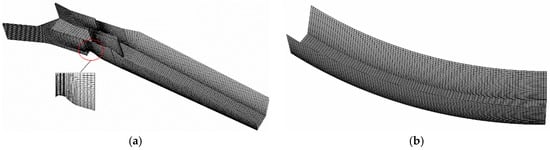
Figure 8.
Schematic of the grid: (a) in the weir crest; and (b) in the curved section of the smooth spillway.
The vertical velocity at position [x = 1.4, y = 0, z = −0.3] of the smooth spillway for three distances was used to test mesh independence, as shown in Figure 9. H stands for the wall height. As can be seen from Figure 9, the velocity distribution in the region of obeys a logarithmic law for and . The velocity in the region of , which is filled with air or a portion of water in a cell, is in accordance with the rule of the air–water interface given by Chanson et al. [26]. For , the distribution of velocity in deviates from the logarithmic law. The relative error of velocity at the first node between and is 3.62%. Thus, for the step and smooth spillway, the distance = 3.5 mm was adopted, and the numbers of total elements for the geometric model were 867,240 and 731,455, respectively.
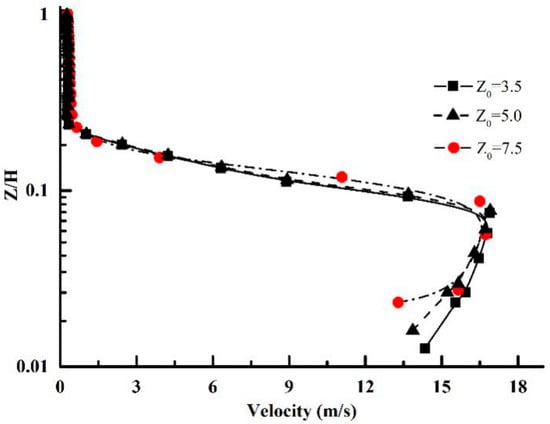
Figure 9.
The vertical velocity at position [x = 1.4, y = 0, z = −0.3] of the smooth spillway for , , and .
Figure 10 shows the flow pattern on the weir crest of the smooth spillway and the curved section measured by the experiment, and the numerically simulated shape of the free water surface. The numerical simulation successfully captured the water wing formed at the pier, and the area not covered by water on the base plate in the curved section was basically consistent with the experimentally measured range. Therefore, the VOF method can successfully simulate the important hydraulic characteristics of free water surface.
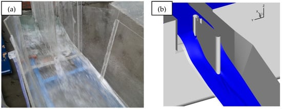
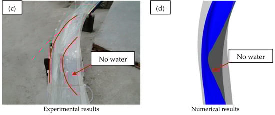
Figure 10.
The experimentally measured (left) and numerically simulated (right) flow regime. (a) and (b) are located on the weir crest and (c,d) are located in the curved section.
The flow pattern from step No. 21 to step No. 24 is shown in Figure 11, which further verifies the reliability of the flow characteristics of the curved spillway with non-uniform-height steps simulated by the numerical model in this study. Figure 11a shows that the water flow on the steps presents the skimming flow regime. The results of the numerical simulation clearly show that the free surface of the flow is relatively smooth, and that air is entrained in the water on the steps. These flow characteristics captured by the numerical model in this study are similar to our experimental results and those described by Chanson et al., Tabbara et al. [27] and Chatila et al. [28] on the skimming flow.
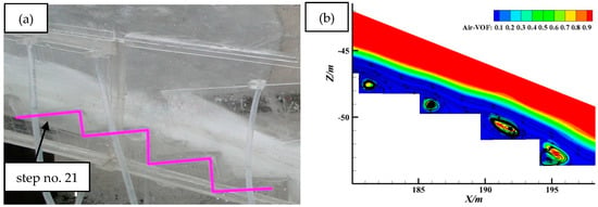
Figure 11.
Flow pattern on the steps. (a) The experimental measurement results; and (b) numerical results. VOF: volume-of-fluid.
Figure 12 shows the computed water level along the path compared to the corresponding measured data. When the volume fraction of water (F) is 0.55, the water level on the concave bank and the convex bank calculated by the numerical simulation is in good agreement with the measured data. Therefore, the VOF method can be used to accurately simulate the profile of the free surface, and the isosurface of a water volume fraction (F) of 0.55 is taken as the profile of free surface [14].
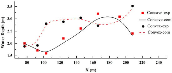
Figure 12.
The water depth in the experimental measurement (exp) and numerical simulation (com).
Figure 13 gives a comparison of the flow velocity near the concave bank, the convex bank, and the central axis on the cross-section as determined by numerical simulation and experiment. As can be seen from Figure 13, under the influence of centrifugal force, the velocity on the concave bank is greater than that on the convex bank, and the flow velocity calculated by numerical simulation is slightly larger than that of the experimental measurement at this point. The maximum difference between the velocity obtained in the numerical simulation and that obtained in the experiment is 8.5%, which meets the requirement of engineering accuracy.
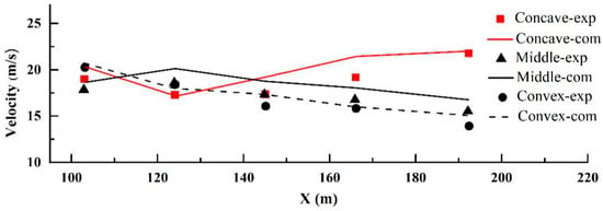
Figure 13.
The water flow velocity obtained by experimental measurement and numerical simulation.
In summary, the VOF model in conjunction with the Re-normalization group (RNG) k-ε turbulence model can successfully simulate the flow and the profile of the free surface. The numerical model is suitable for simulating the flow of the curved spillway with non-uniform-height steps.
4. Results and Discussion
4.1. Main Flow Region
The cross-sectional velocity distributions at the ends of steps Nos. 1, 17, 24, and 28 of the smooth spillway and stepped spillway are shown in Figure 14. The position of the main flow region is analyzed by the velocity distribution in these typical cross-sections.
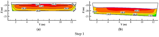
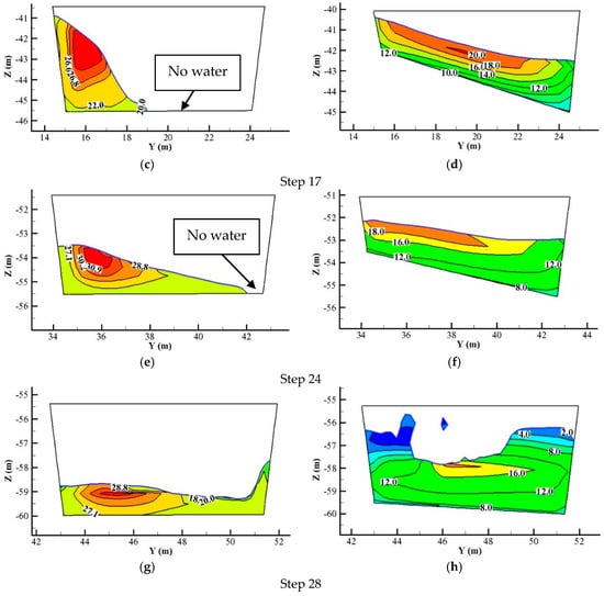
Figure 14.
The cross-sectional velocity distributions at the ends of steps No. 1, 17, 24, and 28 of the smooth spillway and step spillway. (a,c,e,g) are smooth spillways; and (b,d,f,h) are stepped spillways.
Figure 14a,b show the flow velocity distribution of step No. 1 for both spillways. The average velocity of the stepped spillway is lower than that of the smooth spillway, which is due to the loss part of the flow energy of the step. However, the flow velocity distribution in the main flow region is relatively uniform.
The cross-section velocity of step No. 17 after the flow into the curved section is shown in Figure 14c,d. Reinauer et al. [29] theoretically and experimentally studied the influence of the approach Froude number (Fr) on the maximum standing wave heights. For moderate and large Froude numbers (Fr = 4 and 6), the uneven distribution separate bend flow on the cross-section resulted in extremely high-water levels. These hydraulic phenomena were only observed in Figure 14c, in which the severe situation of the base plate of the convex bank not having water cover occurred, while the water flow was completely concentrated on the concave bank, making the water level extremely high. When the non-uniform-height steps were arranged on the smooth spillway, the flow velocity in the main flow region and the water level on both sides were more uniform, which improved the bad flow pattern in the smooth spillway, as seen in Figure 14d.
The velocity at step No. 24, shown in Figure 14e,f, is located where the water flows out of the curved section and into the chute rear section. The base plate of the smooth spillway was still completely uncovered by water, and the main flow region deviated seriously to the concave bank. However, after the non-uniform-height step was arranged, the main flow region was evenly distributed.
Step No. 28 is the last step and is the section where the water flows into the stilling basin. The velocity distribution in this section is shown in Figure 14g,h. As can be seen from Figure 14g,h, the water velocity in the smooth spillway into the stilling basin was very large, reaching about 30 m/s. However, the maximum flow velocity of the curved stepped spillway reached 18 m/s. Therefore, the flow velocity along the path decreased significantly. Additionally, the water level of the curved stepped spillway (2.0 m) was significantly higher than that of the smooth spillway (1.0 m), indicating that the water depth in the stilling basin was increased.
Through the analysis of the main flow region, it was found that the base plate was no longer uncovered by water, and the velocity along the path was significantly reduced after the non-uniform-height steps were placed in the curved spillway. The flow pattern of the water flowing into the stilling basin was improved.
4.2. Flow Pattern on a Step
The velocity fields at step No. 17 are presented in Figure 15 in order to demonstrate the water flow pattern on the steps. The flow patterns on the other steps are all similar.
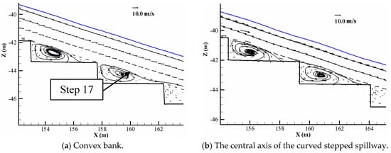
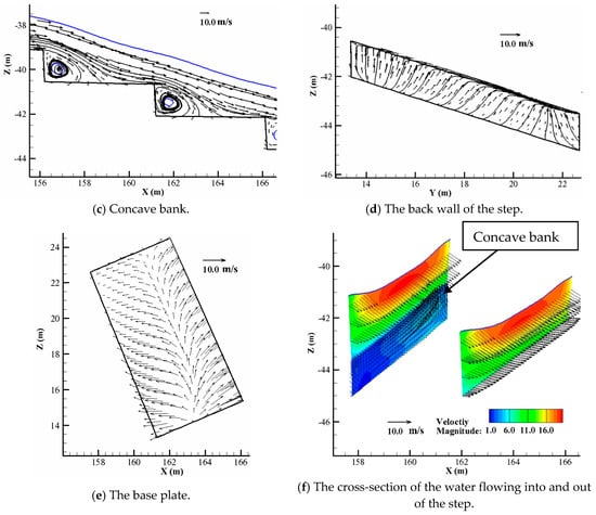
Figure 15.
The velocity field at step No. 17.
The velocity fields in the convex bank, the central axis, and the concave bank are shown in Figure 15a–c. The water flowed down the stepped face, formed a coherent stream that skimmed over the steps and was cushioned by the recirculating fluid trapped between them, and the flow pattern was skimming flow. This is consistent with the description of the air–water phase flow on a stepped spillway by Rajaratnam and Chamani [30,31]. A wide and stable vortex region was formed in the triangular area between the back wall of the step and the base plate. The flow in this vortex area was more disordered, which enhanced the momentum exchange and energy loss. The air was entrained in the water flow in the vortex area of the concave bank. Additionally, the flow velocity on the concave bank of the step was significantly higher than that on the convex bank, and the flow velocity gradually increased from the convex bank to the concave bank.
Figure 15d,e describes the velocity vector distribution of the back wall and the base plate of the step. The flow velocity near the back wall and the base plate was low. The upward flow from the bottom of the water body to the free surface was formed on the back wall. The transverse flow from the concave bank to the convex bank was formed on the base plate, which was caused by the base plate of the concave bank elevated. When the transverse flow was deflected by the convex bank, a stable lateral recirculation zone was formed near to the bank, as shown in Figure 15f.
The results of the velocity field analysis show that the flow pattern was skimming flow, and two stable recirculation zones existed along the path and the transverse. Due to the existence of the recirculation zones, a 3D energy dissipation region on the step was formed, which enhanced the energy dissipation.
4.3. Cavitation Characteristics
Compared with the smooth spillway, the stepped spillway is less prone to cavitation damage. However, for skimming flow on the stepped spillway, a high-intensity shear layer is formed along the connecting consecutive step tips. The flow structure within this shear layer supports cavitation formation along secondary flow features. Iyer et al. [32] and O’Hern [33] studied the development and inception of cavitation in this shear layer experimentally. The above velocity fields indicate that the flow pattern in this study is exactly the skimming flow, and an obvious secondary flow existed on the steps. Therefore, cavitation characteristics of the step must be considered.
Brennen [34] explained in detail the mechanism of cavitation—that is, when the pressure in a local region falls suddenly below the vaporization pressure corresponding to the water temperature in the region, part of the flow starts to vaporize to form a gas phase. Cavitation occurs when these gases escape. Frizell et al. [35] give the cavitation index related to the pressure in Equation (11):
where is absolute pressure, is vapor pressure, is the water density, and is mean velocity.
According to Equation (11), the pressure distribution can preliminarily predict the position and probability of cavitation damage. Chen et al. [36] simulated the pressure distribution on the stepped spillway, which was basically consistent with the data measured by experiment.
Whether or not cavitation may occur in the stepped spillway is determined by Equation (12):
where is incipient cavitation index.
The pressure isolines on step No. 17 are shown in Figure 16, and the pressure distribution on other steps is similar. The triangle region near to the concave bank on the base plate had negative pressure, as shown in Figure 16a. This region had a small range, and the maximum negative pressure value in the region reached 34 kPa. The negative pressure in this region was caused by the fully developed and stable secondary flow, which is consistent with the experimental results of Juny et al. [37] and Sanchez-Juny et al. [38].
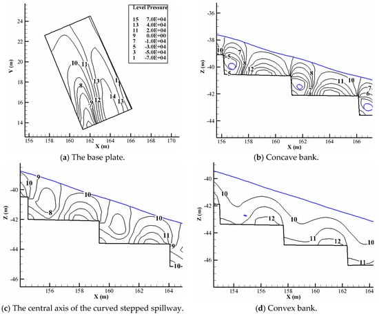
Figure 16.
Pressure isolines on step No. 17 (unit: Pa).
Figure 11b, c respectively show the pressure distribution in the concave bank and the central axis. The negative pressure decreases gradually from the concave bank (34 kPa) to the central axis (6.3 kPa). The pressure is positive from the central axis to the convex bank, and is always positive in the convex bank, as shown in Figure 16d.
The negative pressure zone was more likely to induce cavitation according to Equations (11) and (12). Therefore, after the non-uniform-height steps are arranged on the curved spillway, an aeration device should be set in front of the steps to avoid cavitation.
4.4. Energy Loss
The proposed steps with non-uniform heights not only improve the flow state in the curved spillway, but also need to dissipate the energy along the path as much as possible, thus reducing the size of the stilling basin in the downstream. Different flow states correspond to different energy loss estimation methods. Sorensen [4] and Rajaratnam et al. [30] defined three patterns: (1) isolated roughness flow; (2) wake interference flow; and (3) skimming or quasi-smooth flow. The flow pattern on the step in this study is skimming flow. The energy loss of skimming flow was estimated using the method proposed by Ohtsu et al. [39].
The energy of the curved stepped spillway is:
where is the water depth at the toe of the stepped curved spillway and is the mean velocity. The results of Shvainshtein [5] indicate that total energy losses within a stepped spillway can be considered by the mean velocity.
The energy of the smooth curved spillway is:
where and are the corresponding water depth and mean velocity at the toe of the smooth curved spillway, respectively.
The relative energy loss is defined by Equation (15):
In Equations (13) and (14), the water depth and mean velocity are both numerical values on the cross-section of step No. 28, and the water flows out from the end of step No. 28 directly into the stilling basin.
The relative energy losses are given in Table 6. The energy loss of the stepped spillway is about 44% more than that of the smooth spillway. From the above discussion, the stable vortex formed by shear stress dissipated part of the energy, which is the main form of energy loss. For the curved spillway with the step with non-uniform heights at the bottom, a 3D energy dissipation area was formed due to the transverse velocity, and the flow was sufficiently turbulent to enhance the energy loss along the path.
Table 6.
Relative energy loss of the curved spillway.
5. Conclusions
The reservoir’s shore spillway must be arranged in a curved shape due to the restriction of topography. The flow in this spillway, from the weir crest to the spillway, has a high velocity, a low water depth, and has the characteristics of a curved flow. The water depth in the cross-section was not evenly distributed due to centrifugal force in the curved section, the concave bank was usually larger than the convex bank, and some areas on the base plate were not covered by water. The step with non-uniform heights at the bottom proposed in this study was placed in the smooth curved spillway of this reservoir to improve the flow characteristics. The position of a main flow region, the velocity field and pressure distribution, and the energy loss rate of steps were studied by experiments and numerical simulation.
The non-uniform-height step, which was elevated at the bottom of the concave bank, effectively balanced the partial centrifugal force in the curved section and significantly improved the position of the main flow region. The water flow along the cross-section direction was more uniform, and the adverse water flow phenomenon of the base plate not being covered by water was eliminated completely. Additionally, the maximum velocity of water flowing into the stilling basin decreased from 30 to 18 m/s, and the average water depth increased from 1 to 2 m, which significantly improved the flow regime of water flowing into the stilling basin.
The flow pattern on the steps presented a skimming flow. The water flowed down the stepped face and formed a coherent stream that skimmed over the steps and a stable and fully developed vortex region (secondary recirculation flow region) along the connecting step tips. Owing to the different elevation of the base plate, the water flow from the concave bank to the convex bank also formed a transverse flow, which constituted a 3D energy dissipation region. Comparing the relative energy loss of the stepped spillway with that of the smooth spillway, the energy loss of the stepped spillway was greater by 66%. Therefore, the steps effectively dissipated parts of the energy.
The triangular region near to the concave bank on the base plate had negative pressure, which easily led to cavitation. It is therefore necessary to examine the placement of an aeration device. Additionally, this study only verified the feasibility of this type of step in the project through the case, and the detailed design method was not given, which can be further improved upon in future work.
Author Contributions
Conceptualization: D.L. and G.D.; Methodology: Q.Y.; Software, D.L.; Validation: D.L., Q.Y. and X.M.; Formal Analysis: G.D.; Investigation: D.L.; Resources: Q.Y.; Data Curation: X.M.; Writing—Original Draft Preparation: D.L.; Writing—Review and Editing: X.M.; Visualization: Q.Y.; Supervision: Q.Y.; Project Administration: Q.Y.; and Funding Acquisition: G.D.
Funding
This APC was funded by G.D.
Conflicts of Interest
The authors declare no conflicts of interest.
References
- Ye, J.; McCorquodale, J.A. Simulation of curved open channel flows by 3D hydrodynamic model. J. Hydraul. Eng. 1998, 124, 687–698. [Google Scholar] [CrossRef]
- Chanson, H. Hydraulics of skimming flows over stepped channels and spillways. J. Hydraul. Res. 1994, 32, 445–460. [Google Scholar] [CrossRef]
- Chinnarasri, C.; Wongwises, S. Flow Patterns and Energy Dissipation over Various Stepped Chutes. J. Irrig. Drain. Eng. 2006, 132, 70–76. [Google Scholar] [CrossRef]
- Sorensen, R.M. Stepped spillway hydraulic model investigation. J. Hydraul. Eng. 1985, 111, 1461–1472. [Google Scholar] [CrossRef]
- Shvainshtein, A.M. Stepped spillways and energy dissipation. Hydrotech. Constr. 1999, 33, 275–282. [Google Scholar] [CrossRef]
- Christodoulou, G.C. Energy dissipation on stepped spillways. J. Hydraul. Eng. 1993, 119, 644–650. [Google Scholar] [CrossRef]
- Felder, S.; Chanson, H. Energy dissipation down a stepped spillway with nonuniform step heights. J. Hydraul. Eng. 2011, 137, 1543–1548. [Google Scholar] [CrossRef]
- Pegram, G.G.S.; Officer, A.K.; Mottram, S.R. Hydraulics of skimming flow on modeled stepped spillways. J. Hydraul. Eng. 1999, 125, 500–510. [Google Scholar] [CrossRef]
- Ostad Mirza, M.J.; Matos, J.; Pfister, M.; Schleiss, A.J. Effect of an abrupt slope change on air entrainment and flow depths at stepped spillways. J. Hydraul. Res. 2017, 55, 362–375. [Google Scholar] [CrossRef]
- Meireles, I.C.; Bombardelli, F.A.; Matos, J. Air entrainment onset in skimming flows on steep stepped spillways: An analysis. J. Hydraul. Res. 2014, 52, 375–385. [Google Scholar] [CrossRef]
- Zhang, G.; Chanson, H. Hydraulics of the developing flow region of stepped spillways. II: Pressure and velocity fields. J. Hydraul. Eng. 2016, 142, 04016016. [Google Scholar] [CrossRef]
- Chen, Q.; Dai, G.; Liu, H. Volume of fluid model for turbulence numerical simulation of stepped spillway overflow. J. Hydraul. Eng. 2002, 128, 683–688. [Google Scholar] [CrossRef]
- Ye, M.; Wu, C.; Chen, Y.; Zhou, Q. Case study of an S-shaped spillway using physical and numerical models. J. Hydraul. Eng. 2006, 132, 892–898. [Google Scholar] [CrossRef]
- Tabbara, M.; Chatila, J.; Awwad, R. Computational simulation of flow over stepped spillways. Comput. Struct. 2005, 83, 2215–2224. [Google Scholar] [CrossRef]
- Toro, J.P.; Bombardelli, F.A.; Paik, J. Detached eddy simulation of the nonaerated skimming flow over a stepped spillway. J. Hydraul. Eng. 2017, 143, 04017032. [Google Scholar] [CrossRef]
- Toro, J.P.; Bombardelli, F.A.; Paik, J.; Meireles, I.; Amador, A. Characterization of turbulence statistics on the non-aerated skimming flow over stepped spillways: A numerical study. Environ. Fluid Mech. 2016, 16, 1195–1221. [Google Scholar] [CrossRef]
- Rozovskiĭ, I.L. Flow of Water in Bends of Open Channels; Academy of Sciences of the Ukrainian SSR: Kiev, Ukraine, 1957. [Google Scholar]
- Wu, Y.F.; Zhu, J.Y. Exposed bottom phenomenon of curved channels with rapid flows. Adv. Sci. Technol. Water Resour. 2011, 31, 9–12. (In Chinese) [Google Scholar]
- Rodi, W. Turbulence Models and Their Application in Hydraulics; Routledge: London, UK, 2017. [Google Scholar]
- Hirt, C.W.; Nichols, B.D. Volume of fluid (VOF) method for the dynamics of free boundaries. J. Comput. Phys. 1981, 39, 201–225. [Google Scholar] [CrossRef]
- Cheng, X.; Chen, Y.; Luo, L. Numerical simulation of air-water two-phase flow over stepped spillways. Sci. China Ser. E Technol. Sci. 2006, 49, 674–684. [Google Scholar] [CrossRef]
- Boes, R.M.; Hager, W.H. Two-phase flow characteristics of stepped spillways. J. Hydraul. Eng. 2003, 129, 661–670. [Google Scholar] [CrossRef]
- Li, D.; Yang, Q.; Ma, X.; Dai, G. Free Surface Characteristics of Flow around Two Side-by-Side Circular Cylinders. J. Mar. Sci. Eng. 2018, 6, 75. [Google Scholar] [CrossRef]
- Jin, X.; Lin, P. Viscous effects on liquid sloshing under external excitations. Ocean Eng. 2018. [Google Scholar] [CrossRef]
- Pope, S.B. Turbulent Flows; Cambridge University Press: Cambridge, UK, 2001. [Google Scholar]
- Chanson, H.; Brattberg, T. Experimental Study of the Air-Water Shear Flow in a Hydraulic Jump. Int. J. Multiph. Flow 2000, 26, 583–607. [Google Scholar] [CrossRef]
- Chanson, H. Hydraulics of skimming flows on stepped chutes: The effects of inflow conditions? J. Hydraul. Res. 2006, 44, 51–60. [Google Scholar] [CrossRef]
- Chatila, J.; Tabbara, M. Computational modeling of flow over an ogee spillway. Comput. Struct 2004, 82, 1805–1812. [Google Scholar] [CrossRef]
- Reinauer, R.; Hager, W.H. Supercritical bend flow. J. Hydraul. Eng. 1997, 123, 208–218. [Google Scholar] [CrossRef]
- Rajaratnam, N. Skimming flow in stepped spillways. J. Hydraul. Eng. 1990, 116, 587–591. [Google Scholar] [CrossRef]
- Chamani, M.R.; Rajaratnam, N. Characteristics of skimming flow over stepped spillways. J. Hydraul. Eng. 1999, 125, 361–368. [Google Scholar] [CrossRef]
- Iyer, C.O.; Ceccio, S.L. The influence of developed cavitation on the flow of a turbulent shear layer. Phys. Fluids 2002, 14, 3414–3431. [Google Scholar] [CrossRef]
- O’Hern, T.J. An experimental investigation of turbulent shear flow cavitation. J. Fluid Mech. 1990, 215, 365–391. [Google Scholar] [CrossRef]
- Brennen, C.E. Cavitation and Bubble Dynamics; Cambridge University Press: Cambridge, UK, 2013. [Google Scholar]
- Frizell, K.W.; Renna, F.M.; Matos, J. Cavitation potential of flow on stepped spillways. J. Hydraul. Eng. 2012, 139, 630–636. [Google Scholar] [CrossRef]
- Chen, Q.; Dai, G.; Liu, H. Turbulence numerical simulation for the stepped spillway overflow. Tianjin Daxue Xuebao/J. Tianjin Univ. Sci. Technol. 2002, 35, 23–27. [Google Scholar]
- Juny, M.S.; Pomares, J.; Dolz, J. Pressure field in skimming flow over a stepped spillway. In Proceedings of the International Workshop on Hydraulics of Stepped Spillways, Zurich, Switzerland, 22–24 March 2000; Minor, H.E., Hager, W.H., Eds.; AA Balkema: Rotterdam, The Netherlands, 2000; pp. 137–146. [Google Scholar]
- Sanchez-Juny, M.; Blade, E.; Dolz, J. Pressures on a stepped spillway. J. Hydraul. Res. 2007, 45, 505–511. [Google Scholar] [CrossRef]
- Ohtsu, I.; Yasuda, Y.; Takahashi, M. Flow characteristics of skimming flows in stepped channels. J. Hydraul. Eng. 2004, 130, 860–869. [Google Scholar] [CrossRef]


© 2018 by the authors. Licensee MDPI, Basel, Switzerland. This article is an open access article distributed under the terms and conditions of the Creative Commons Attribution (CC BY) license (http://creativecommons.org/licenses/by/4.0/).