Investigation of Flow, Erosion, and Sedimentation Pattern around Varied Groynes under Different Hydraulic and Geometric Conditions: A Numerical Study

Abstract

Groynes are popular hydraulic structures often used to control the erosion of banks by altering flow and sediment transport. In this paper, the effects of altering groyne orientation and spatial setup (from large to small and vice versa) on flow patterns, bed erosion, and sedimentation are numerically investigated. Studied groynes were parallel to each other, non-submerged, and impermeable. Numerical simulations were conducted in FLOW-3D. A nested mesh configuration combined with Van-Rijn formula on sediment transport yielded more accurate results when comparing numerical results to experiments. Groynes arranged from large to small at an angle of 45° decreased the scour depth by up to 55%, and an arrangement from small to large at an angle of 135° reduced the scour depth by up to 72%. Additionally, it was observed that simulations with an orientation closer to 90 degrees needed more equilibrium time when compared to other simulations.

1. Introduction

Scouring around hydraulic structures (such as piers, abutments, levee, groynes, etc.) has been one of the most significant problems in their design. Predicting and reducing scour has posed several challenges to engineers in the last decades. In this study, the emphasis is on groynes. These are structures which may be of different shape and length, submerged or non-submerged, deflecting flow current with the purpose of protecting river banks [1]. Several studies have been undertaken on groynes and their influence. For example, Vaghefi, et al. [2] investigated the effect of the shape of groynes on flow pattern. Zaid, et al. [3] looked into groyne materials by studying the effects of stone and wooden groynes in a restored river reach. Uijttewaal [4] tested four types of groynes found among the largest rivers in Europe to determine efficient alternative designs, while considering the physical, economical, and ecological aspects [4]. Other researchers, such as Garde, et al. [5], Melville [6], Saneie [7], Zhang and Nakagawa [8], Ghodsian and Vaghefi [9], Al-Khateeb et al. [10], Radan and Vaghefi [11], and Gualtieri [12] have investigated erosion and sedimentation patterns, scour hole depth, and riverbed stress variation around groynes under various conditions. Through simulation experiments, Uijttewaal et al. [13] studied the exchange processes between a river and its groyne fields. To increase their efficiency, groynes are applied in groups instead. Their inter-distance, length, and height affect performance, which influences factors such as shear stress and subsequently alters the channel morphology. Karami et al. [14], Acharya and Duan [15], Koken and Gogus [16], McCoy et al. [17], and Yossef and Vriend [18] are among researchers to study flow characteristics and scour hole in a group of groynes.

Limitations of physical models and advancements in computational power has increased the adoption of numerical solutions in solving complex flow dynamics and related phenomena. Ning et al. [19] numerically investigated the effects of time on turbulent flows to simulate the scour depth around a single groyne. Abdulmajid et al. [20] studied hydraulic conditions and velocity distribution around L shaped groynes at a river arc utilizing a numerical model. Vaghefi et al. [21] probed local scouring around T shaped groynes in a 90° bend of a channel. Giglou et al. [22] investigated the impacts of various groyne group orientations, lengths, and distances on flow, erosion, and sedimentation patterns.

In the present study, the impacts of varying groyne length and orientation angle on scouring depth in groups of parallel groynes (each group having 3 groynes) of non-equal lengths are investigated. An advanced numerical simulation software, FLOW-3D, is used to simulate the problem, and numerical simulations are validated with laboratory experiments.

2. Governing Equations

Fluid motion equations include conservation of mass and momentum equations (Equations (2)–(4)), which FLOW-3D solves to calculate flow hydraulics. Besides these, FLOW-3D applies the volume of fluid (VOF) equation to ensure that proper boundary conditions are applied at the free surface (Equation (5)).

$$V_F\frac{\partial \rho }{\partial t}+\frac{\partial }{\partial x}\left(\rho u{A}_x\right)+R\frac{\partial }{\partial y}(\rho v{A}_y)+\frac{\partial }{\partial z}\left(\rho w{A}_z\right)=R_{SOR}$$

(1)

$$\frac{\partial u}{\partial t}+\frac{1}{V_F}\left(u{A}_x\frac{\partial u}{\partial x}+v{A}_{y}R\frac{\partial u}{\partial y}+w{A}_z\frac{\partial u}{\partial z}\right)-\xi \frac{A_y{v}^2}{x{V}_F}=-\frac{1}{\rho }\frac{\partial \rho }{\partial x}+G_x+f_x$$

(2)

$$\frac{\partial v}{\partial t}+\frac{1}{V_F}\left(u{A}_x\frac{\partial v}{\partial x}+v{A}_{y}R\frac{\partial v}{\partial y}+w{A}_z\frac{\partial v}{\partial z}\right)-\xi \frac{A_{y}uv}{x{V}_F}=-\frac{R}{\rho }\frac{\partial \rho }{\partial y}+G_y+f_y$$

(3)

$$\frac{\partial w}{\partial t}+\frac{1}{V_F}\left(u{A}_x\frac{\partial w}{\partial x}+v{A}_{y}R\frac{\partial w}{\partial y}+w{A}_z\frac{\partial w}{\partial z}\right)=-\frac{1}{\rho }\frac{\partial \rho }{\partial z}+G_z+f_z$$

(4)

$$V_F\frac{\partial F}{\partial t}+\nabla .\left(AUF\right)=0$$

(5)

where V_F = open volume ratio to flow, $\rho$ = fluid density, (u, v, w) = velocity components in (x, y, z), R_SOR = source function, (A_x, A_y, A_z) = fractional areas, (G_x, G_y, G_z) = gravitational force, (f_x, f_y, f_z) = body force per unit mass in (x, y, z) directions, respectively. The final part of Equations (2) to (4) show mass injection in zero velocity. In Equation (5), A = average flow area, U = average velocity in (x, y, z) direction, and F is volume flow function. When the cell is filled with fluid, the value of F is 1, and when it is empty, F is 0. In FLOW 3D, two methods are utilized for simulations; Volume of Fluid (VOF) and Fractional Area Volume Obstacle Representation (FAVOR) methods [23]. As earlier stated, VOF is used to show the performance of fluid in a free surface and FAVOR is utilized to simulate the surfaces and rigid bodies, such as complex geometric boundaries. To analyze sediment transport, suspended load and bed load are evaluated separately. Suspended load is achieved via the calculation of transient Advection-diffusion equation (ADE) (Equation (6)).

$$\frac{\partial c}{\partial t}+U_i\frac{\partial c}{\partial x_i}+W_s\frac{\partial c}{\partial z}=\frac{\partial }{\partial x_i}\left(\mathsf{\Gamma }\frac{\partial c}{\partial x_i}\right)$$

(6)

In which $c$ is concentration of the suspended load, U is Reynolds-averaged water velocity, Ws is fall velocity of the sediment, x is general space dimension, z is the vertical direction, and $\mathsf{\Gamma }$ is diffusion coefficient (which is the ratio of turbulent viscosity to turbulent Schmidt number). Based on Gualtieri et al. [24], there are no universally accepted values of the Schmidt number.

In near bed cells, the concentration of sediment and bed load are achieved by utilizing van Rijn [25] equations (Equations (7) and (8), respectively):

$$c_{bed}=0.015\ast \frac{d^{0.3}{(\frac{\tau -{\tau }_c}{{\tau }_c})}^{1.5}}{g{(\frac{{\rho }_s-{\rho }_w}{{\rho }_w{\vartheta }^2})}^{0.1}}$$

(7)

In which d is sediment particle diameter, $\tau$ is bed shear stress, ${\tau }_c$ is critical shear stress for the motivation of sediment particles based on Shields diagram, ${\rho }_s$ and ${\rho }_w$ are the sediment particle and water densities, respectively, $\vartheta$ is kinematic viscosity of water, and g is gravitational acceleration. Bed load is evaluated using van Rijn equation:

$$\frac{q_b}{d^{1.5}\sqrt{\frac{{\rho }_s-{\rho }_w}{{\rho }_w}g}}=0.053\ast \frac{{(\frac{\tau -{\tau }_c}{{\tau }_c})}^{1.5}}{d^{0.3}{(\frac{{\rho }_s-{\rho }_w}{{\rho }_w{\vartheta }^2})}^{0.1}}$$

(8)

In which $q_b$ is the bed load.

It should be noted that a correct prediction of sediment transport improves the accuracy of a scour predictive model. For example, Dodaro et al. [26] and Dodaro et al. [27] modified an available sediment transport equation to improve scour depth prediction.

3. Numerical Simulation and Validation

3.1. Laboratory Experiment

Karami, Basser, Ardeshir, and Hosseini [14] constructed a rectangular flume of 14 m length, 1 m width and 1 m depth with poly glass, stabilized with a metal frame, and placed three non-submerged and impermeable groynes of 0.25 m length transverse to flow. They placed the first groyne at 6.16 m from the flume entrance and selected distances twice the length of the groynes. These values were selected based on the recommendations of Zhang [28] and Gisonni et al. [29]. Flow depth was maintained at 0.15 m. The flume was filled with 0.35 m thick uniform sediments having a median size $({\mathrm{d}}_{50})$ of 0.91 mm, specific gravity, ${\mathrm{s}}_{\mathrm{s}}$, of 2.65, and geometric standard deviation, ${\mathsf{\sigma }}_{\mathrm{g}}$, of 1.38. At the beginning of each experiment, the laboratory flume was first gradually filled with water to saturate the bed material. Then the sluice gate located at the end of the flume for controlling water level was raised to achieve the desired discharge (Q). Velocity profile and bed profile changes around the groynes were measured using an Acoustic Doppler Velocimetry (ADV) and a Laser Bed Profiler (LBP), respectively. LBP had an accuracy of ±1 mm in width and ±0.1 mm in depth. As the flow pattern has a significant effect on sediment transport, 50 points of velocity measurements were taken at z = 2 cm above the bed for flow characteristics. Details and results of some experiments utilized for validation are showed in Table 1, whereby Q is flow discharge (m³/s), Y is flow depth (m), U is flow velocity (m/s), U/U_cr is a proportion of flow velocity to critical velocity of Shields, Fr is Froude number, d_s1, d_s2, and d_s3 are maximum scour depth beneath the first, second, and third groynes in meters, respectively, and V represents the eroded sediment volume (m³).

Table 1. Specifications and results of Karami, Basser, Ardeshir, and Hosseini [14] simulation.

Test Number.	Q (m3/s)	Y (m)	U (m/s)	U/Ucr	Fr	ds1 (m)	ds2 (m)	ds3 (m)	V (m3)
E1	0.035	0.150	0.233	0.650	0.190	0.156	0.000	0.026	0.0165

3.2. Numerical Setup

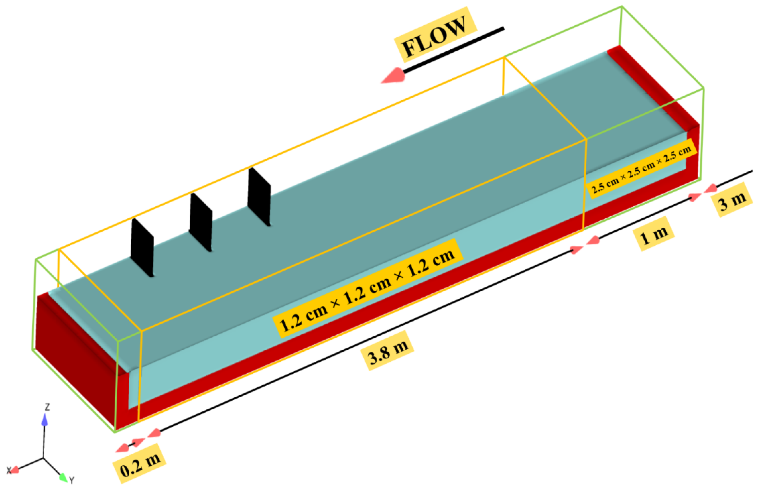
In this study, the flow field was computed by solving the Reynolds-averaged Navier-Stokes equations using the $k-\epsilon$ turbulent closure model. To initialize the model, water depth was fixed at 0.5 m. At the inlet, constant discharge was set to 0.035 m³/s, while a continuative boundary was applied at the outlet. A continuative boundary condition consists of zero normal derivatives at the boundary for all quantities. The zero-derivative condition is intended to represent a smooth continuation of the flow through a boundary [23]. Wall boundary conditions were applied on the sides, and on the remaining sides (bottom and top) a symmetry boundary was assigned (Figure 1).

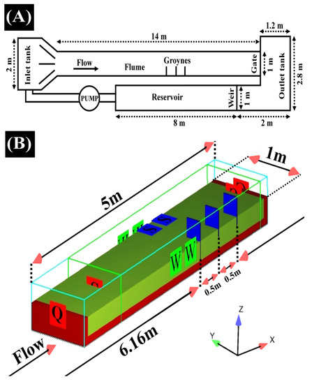
Figure 1. (A) Sketch of laboratory experiment and (B) Utilized Boundary conditions of the numerical simulation.

Based on preliminary investigations, the length of the channel was considered to be 5 m and the distance between 3 m to 8 m was simulated numerically. From 3 m to 6.16 m, where the first groyne was placed, the fully developed current would be formed, and from 7.18 m to 8 m, the vortices of the last groyne would be fully created, making it possible to depict the profile of erosion and sedimentation in the last groyne as well. After initial tests, the nested mesh was found to be the most appropriate simulation for this case. A comparison on scour on the first, second, and third groynes, and the maximum scour depth with experimental data, was made. Two mesh boxes of different size were utilized; closer to the groynes, a finer mesh box was utilized, while farther from the groynes, a coarse mesh box was used (Figure 2). In total, there were 192,000 coarse cells (2.5 cm in all directions) and 1,315,550 fine cells (1.2 cm in all directions). All simulated groynes were within the finer mesh block to fully resolve flow dynamics and enhance accuracy.

Figure 2. Sketch of mesh setup.

Sensitivity analysis was carried out on the mesh size (Table 2). In this Table, d_s1, d_s2, and d_s3 are maximum scour depth at the first, second, and third groynes, respectively. A computer with a Core i7-5820K GHz processor and 32GB RAM was used for the simulations.

Table 2. Mesh size sensitivity analysis.

Test Number	Coarser Mesh Size (m)	Finer Mesh Size (m)	Total Number of Cells	Numerical Simulation			Laboratory Experiment			Computational Time (hour)
				ds1 (m)	ds2 (m)	ds3 (m)	ds1 (m)	ds2 (m)	ds3 (m)
1	0.030	0.020	395880	0.091	0.016	0.020	0.156	0.000	0.026	71
2	0.025	0.012	1507550	0.133	0.005	0.023	0.156	0.000	0.026	146

Sensitivity analysis indicates better results with mesh refinement at a computational cost (Table 2).

3.3. Data Validation

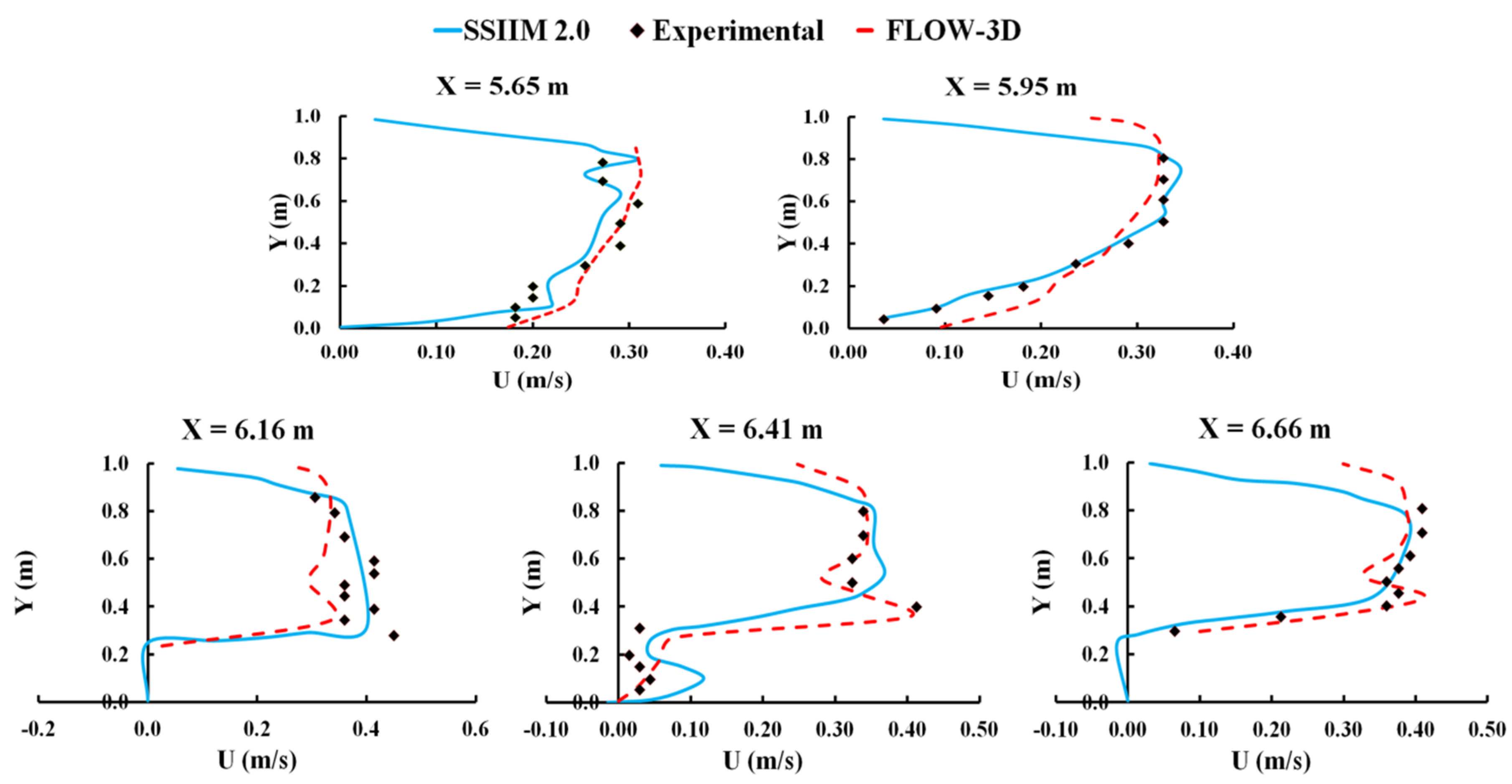
Flow velocity was measured at 50 points in a horizontal plane of z = 2 cm over the bed and at distances 5.65, 5.95, 6.16, 6.41, and 6.66 m from the channel inlet. As Karami, Basser, Ardeshir, and Hosseini [14] chose $k-\epsilon$ RNG turbulence simulation in their numerical simulation, for comparison between FLOW-3D, SSIIM 2.0, and laboratory experiments results, the $k-\epsilon$ RNG turbulence simulation was applied in our study. Comparison of simulated absolute velocity in Computational Fluid Dynamics (CFD) simulations and experimental data is shown in Figure 3 and Table 3.

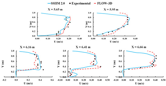
Figure 3. Velocity in horizontal sections; z = 2 cm, x = 5.65, 5.95, 6.16, 6.41, and 6.66m.

Table 3. Comparison of simulated absolute velocity in Computational Fluid Dynamics (CFD) simulation and experimental data.

Cross Section	FLOW-3D	SSIIM 2.0	FLOW-3D	SSIIM 2.0
	* R2	R2	** RMSE	RMSE
X = 5.65m	0.776	0.790	0.031	0.022
X = 5.95m	0.960	0.970	0.055	0.019
X = 6.16m	0.428	0.157	0.117	0.078
X = 6.41m	0.819	0.858	0.071	0.066
X = 6.66m	0.897	0.967	0.038	0.051

Note: * R² is Coefficient of determination and ** RMSE is Root mean square error.

The differences between numerical and experimental observation may be due to complexities of flow pattern and vortexes, or other factors that are not considered in the turbulence formula. At some cross-sections differences are seen, which would be the result of complexities and high vortex intensities. Nonetheless, based on the accuracy parameters applied (R² and RMSE in Table 3), the numerical results are acceptable.

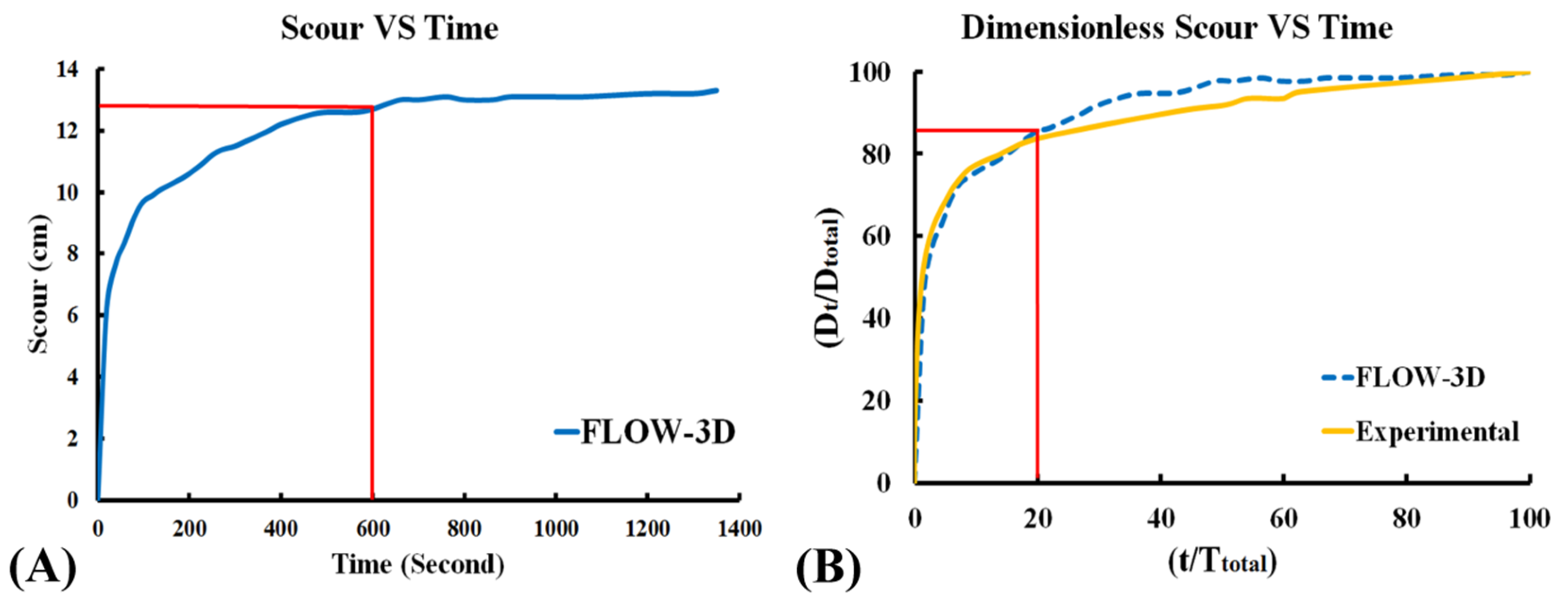
The laboratory experiments of Karami, Basser, Ardeshir, and Hosseini [14], using Chiew [30] criterion, reached their equilibrium state in 3000 min. Hence, a change in bed elevation of less than 1% during 15% of the modelling time was set to be the simulation stop time criterion. Based on the scouring-time chart of the numerical simulation (Figure 4A), the simulation equilibrium was evident, and the modeling time was therefore set to 1350 s.

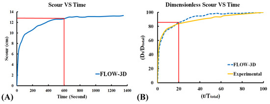
Figure 4. Scouring-time chart.

Comparison of two numerical and laboratory experiments was performed using dimensionless time. The scouring process chart in the experimental work of Karami, Basser, Ardeshir, and Hosseini [14], Jahangirzadeh et al. [31], and numerical simulation of this paper is shown in Figure 4B.

Comparison of the two charts shows good performance of the numerical simulation in simulating the scouring process. The charts further show that more than 85% of scouring occurred within 20% of the scouring time, and until that time, the experiment and numerical results are almost overlapping. Equilibrium scour is reached after 600 s, as shown in Figure 4A.

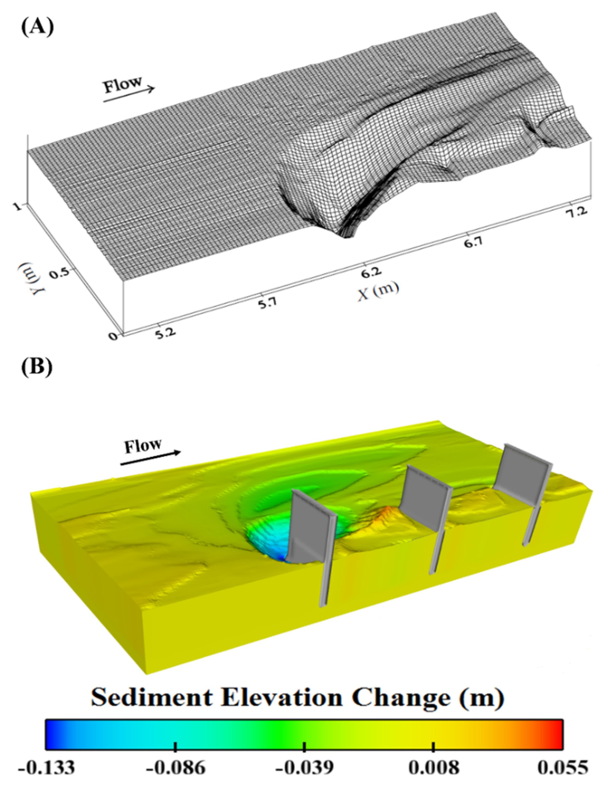
After the equilibrium state, the maximum scour in FLOW-3D was slightly underestimated at 0.133 m when compared to the maximum scour of 0.156 m from the laboratory experiments. The scour pattern is shown in Figure 5.

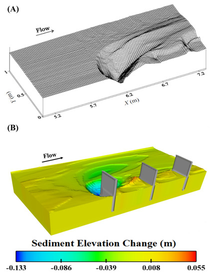
Figure 5. Bed elevation changes from (A) laboratory experiments and (B) FLOW-3D.

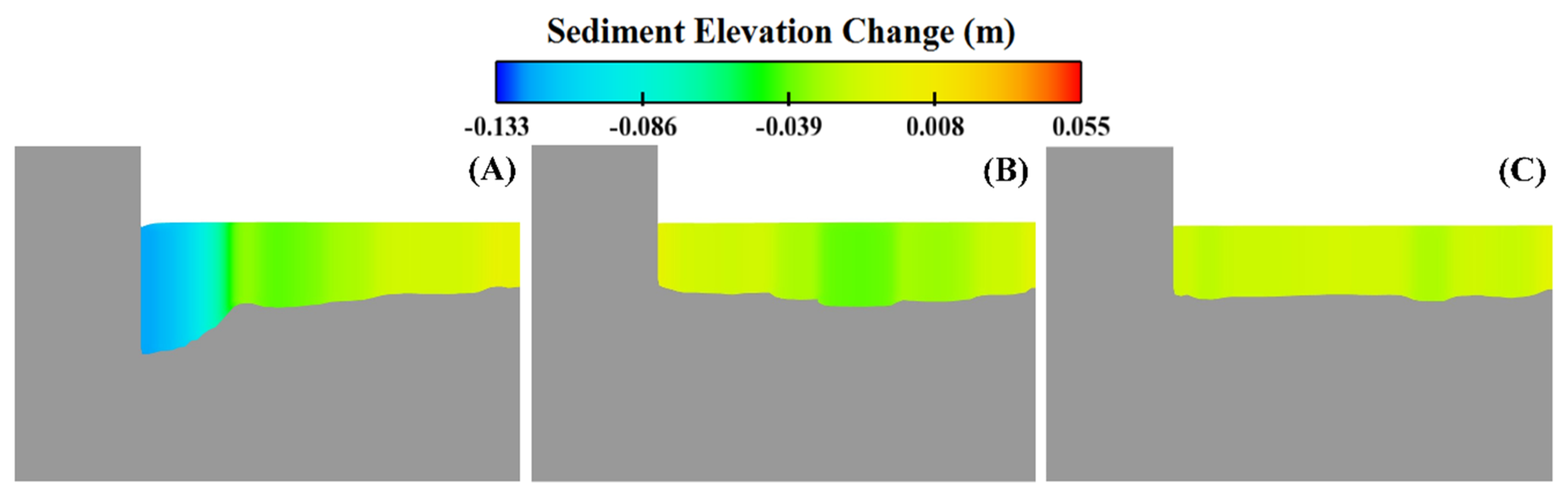
Figure 6 and Table 4 show the maximum scour beneath the first, second, and third groyne of 0.133 m, 0.005 m, and 0.023 m, respectively.

Figure 6. Scour beneath (A) first, (B) second, and (C) third groynes.

Table 4. Maximum scour comparison beneath the three groynes between FLOW-3D and experimental results [14].

	ds3(m)	ds2(m)	ds1(m)
Experimental	0.026	0.0	0.156
FLOW-3D	0.023	0.005	0.133

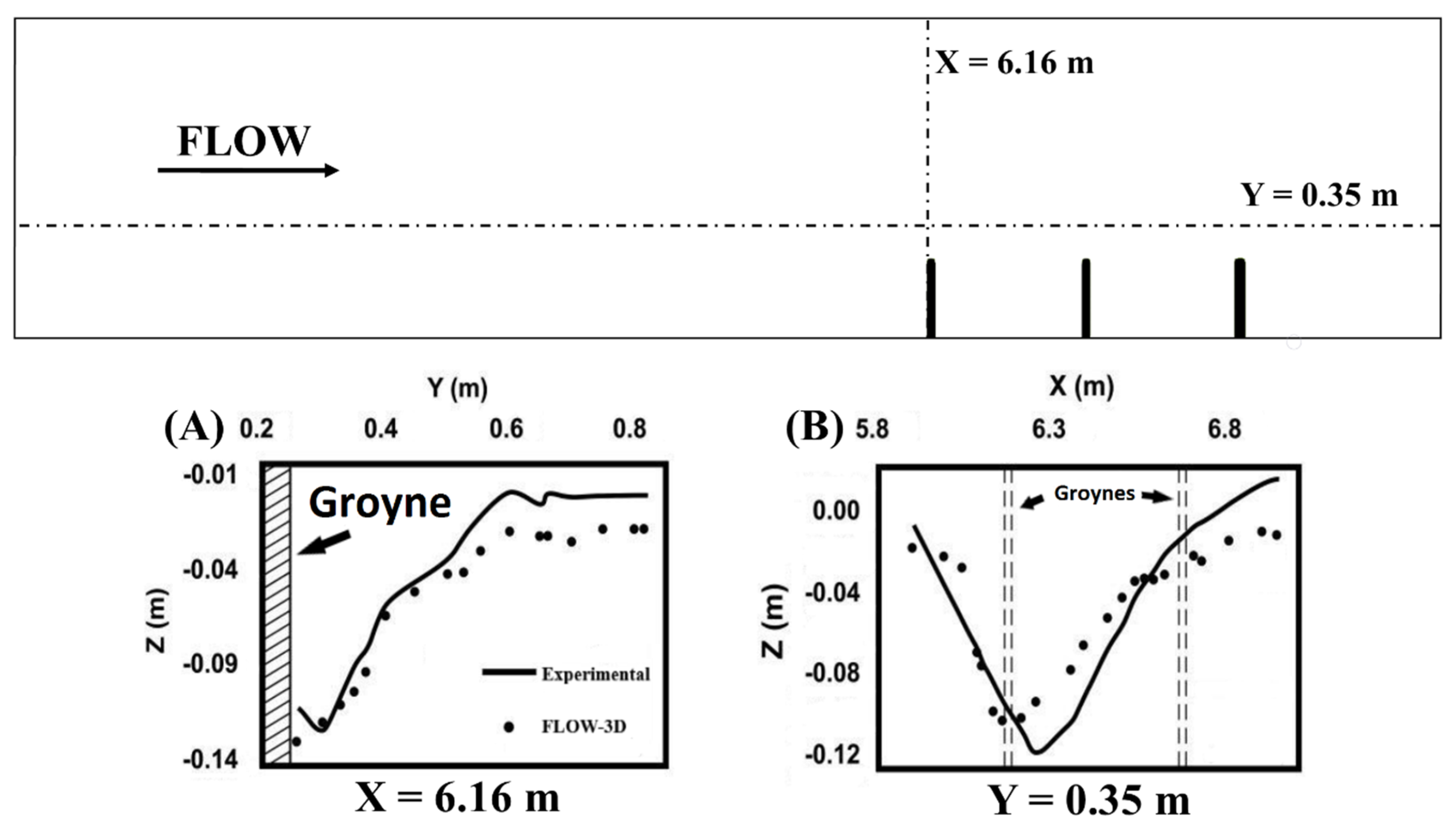
To monitor bed elevation changes, four cross- and longitudinal sections after the constriction were selected, from which 160 points were monitored. In Figure 7, the scour depth at a cross- and longitudinal section around the groyne is shown for both laboratory experiment and the numerical simulation (about 20 points per section). Three statistical parameters were used for assessment, including a coefficient of determination (R²) = 0.91, mean absolute error (MAE) = 0.0162, and root mean squared error (RMSE) = 0.0214. Despite the slight differences in bed elevation changes between FLOW-3D and the experimental data in Figure 7, statistical parameters suggest satisfactory results.

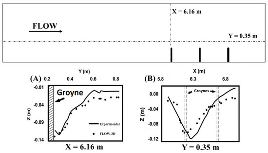
Figure 7. Experiment and FLOW-3D scour profiles, (A) cross section at x = 6.16 m, (B) longitudinal section at y = 0.35 m.

3.4. Numerical Simulations Description of Groynes with Different Length and Orientations

To understand the influence of orientation and length variation, 15 simulations (Table 5) were used, in which three parallel impermeable and non-submerged groynes with distances of 60 cm and 3 cm thickness were located. Groynes in the table were of the same length (30 cm) and were located on the flow route at an angle of 90°. This simulation served as a reference simulation for other cases. All the angles are measured from downstream and vary between 45° and 135° to maintain a constriction ratio of less than 25%.

Table 5. Characteristics of the simulations.

Simulation Number.	Simulation Description	Groynes Orientation (with Respect to Flow Direction) in (°)	First Groyne Length (cm)	Second Groyne Length (cm)	Third Groyne Length (cm)	Constriction Ratio (%)
1	90D.30.30.30	90	30	30	30	30
2	45D.20.30.40	45	20	30	40	28
3	60D.20.30.40	60	20	30	40	35
4	75D.20.30.40	75	20	30	40	37
5	90D.20.30.40	90	20	30	40	40
6	105D.20.30.40	105	20	30	40	37
7	120D.20.30.40	120	20	30	40	35
8	135D.20.30.40	135	20	30	40	28
9	45D.40.30.20	45	40	30	20	28
10	60D.40.30.20	60	40	30	20	35
11	75D.40.30.20	75	40	30	20	37
12	90D.40.30.20	90	40	30	20	40
13	105D.40.30.20	105	40	30	20	37
14	120D.40.30.20	120	40	30	20	35
15	135D.40.30.20	135	40	30	20	28

Note: D is degrees.

In the second to eigth simulations, the groynes were arranged in the order 20, 30, and 40 cm length from the first to third groyne, respectively. In order to investigate the impacts of groyne arrangement, in simulations 9 to 15, groynes were arranged in the reverse order, with the first groyne being 40 cm and the last 20 cm. These cases are placed at angles (45°, 60°, 75°, 90°, 105°, 120°, and 135°) similar to the previous arrangement. In all the simulations, the simulation setup was similar to that of validation.

4. Results

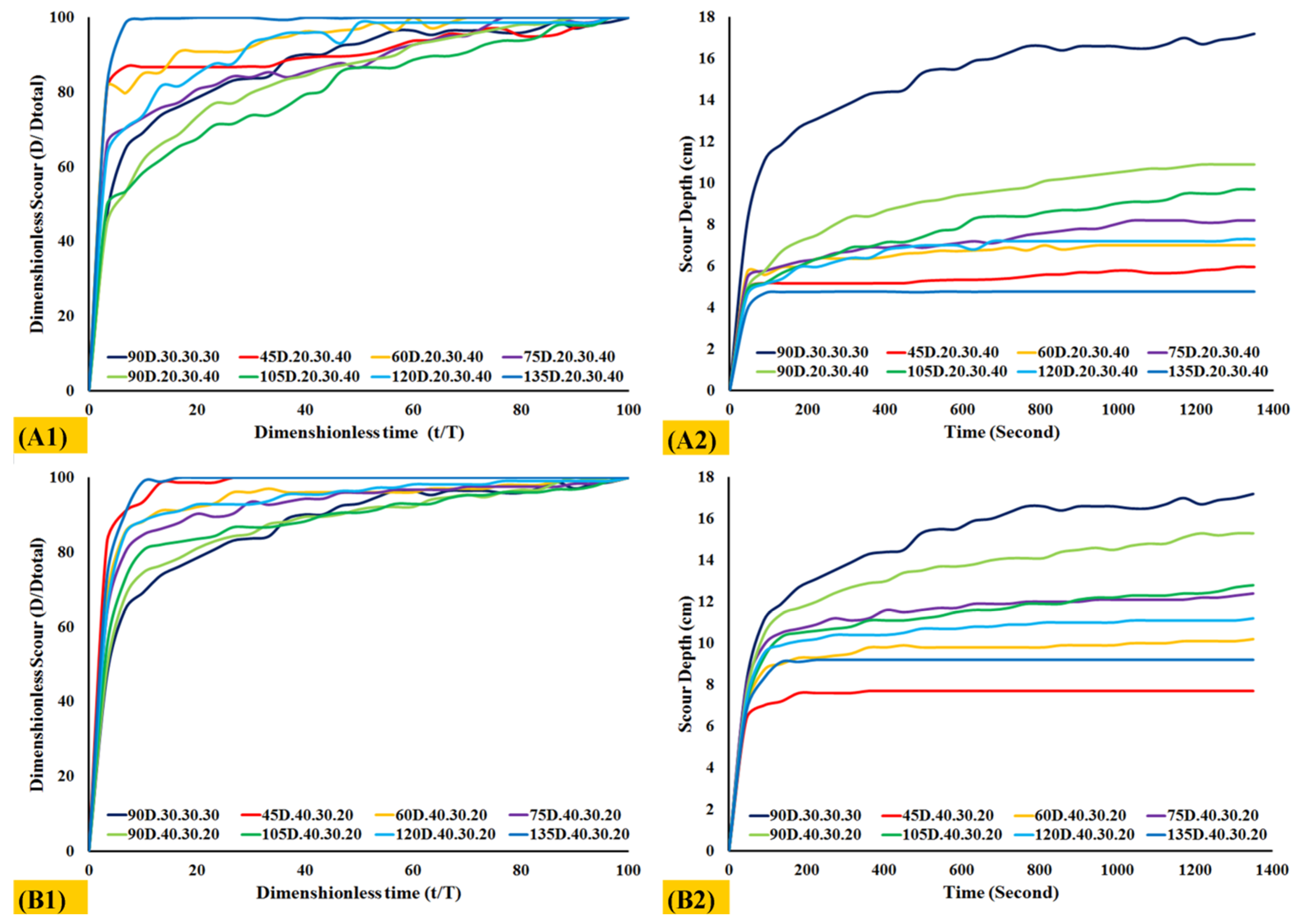
Figure 8 shows the scour equilibrium times and the dimensionless scour versus time in simulation 1/15, indicating that more than 50% of erosion occurred in the first 10% of the total simulation time. Simulations 5 and 6 achieved their equilibrium time later when compared to other simulations.

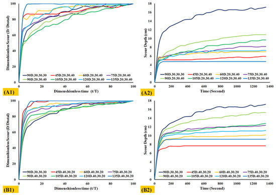
Figure 8. (A1) Dimensionless scour versus time in the simulation 2/8. (A2) Scour depth versus time in the simulation 2/8. (B1) Dimensionless scour versus time in the simulation 1/9. (B2) Scour depth versus time in the simulation 1/9. D is maximum scour depth at each time and D_total is maximum scour depth at the end of the simulation time.

Numerical results indicate continued scouring in some simulations after 1350 s, such as in simulation 1, 5, 6, and 12. The simulation scour equilibrium time considered 1350 s because of computational time and the validation part.

In other simulations, more than 70% of scour occurred within 19% of the simulation time. In simulations 9/15, about 70% of scour occurred within 10% of the simulation time. It is evident from all the simulations that the equilibrium time is less than that of the reference simulation. In all the groyne arrangement, it is observed that as the angle of the groynes approached 90°, the equilibrium time increased. Groynes arranged in an ascending order reached an equilibrium state earlier than their counterparts. Scour depth and sedimentation in the first, second, and third groynes are shown in Table 6.

Table 6. Scouring results from the simulation 1/15.

Simulation Number.	Simulation Description	Maximum Scour Depth (cm)			Maximum Scour Depth (cm)	Maximum Deposition Depth (cm)
S		First Groyne	Second Groyne	Third Groyne
1	90D.30.30.30	17.2	2.78	4.61	17.2	5.80
2	45D.20.30.40	5.96	4.27	5.42	5.96	2.19
3	60D.20.30.40	7.00	4.77	6.96	7.00	2.51
4	75D.20.30.40	8.20	4.48	7.51	8.20	2.22
5	90D.20.30.40	10.90	4.77	6.15	10.90	3.00
6	105D.20.30.40	9.70	3.79	6.82	9.70	1.95
7	120D.20.30.40	7.30	2.68	5.96	7.30	2.96
8	135D.20.30.40	4.77	2.08	3.66	4.77	1.67
9	45D.40.30.20	7.70	2.41	2.50	7.70	2.93
10	60D.40.30.20	10.20	2.12	2.51	10.20	3.73
11	75D.40.30.20	12.40	0.35	2.37	12.40	5.39
12	90D.40.30.20	15.30	0.10	1.90	15.30	4.53
13	105D.40.30.20	12.80	−0.10	2.56	12.80	4.23
14	120D.40.30.20	11.20	0.00	1.72	11.20	4.59
15	135D.40.30.20	9.20	0.65	1.80	9.20	2.26

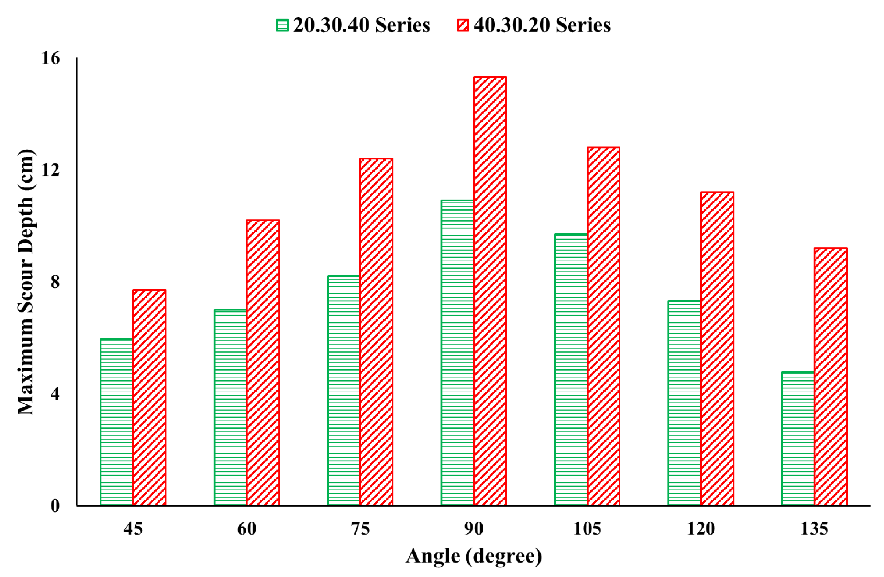
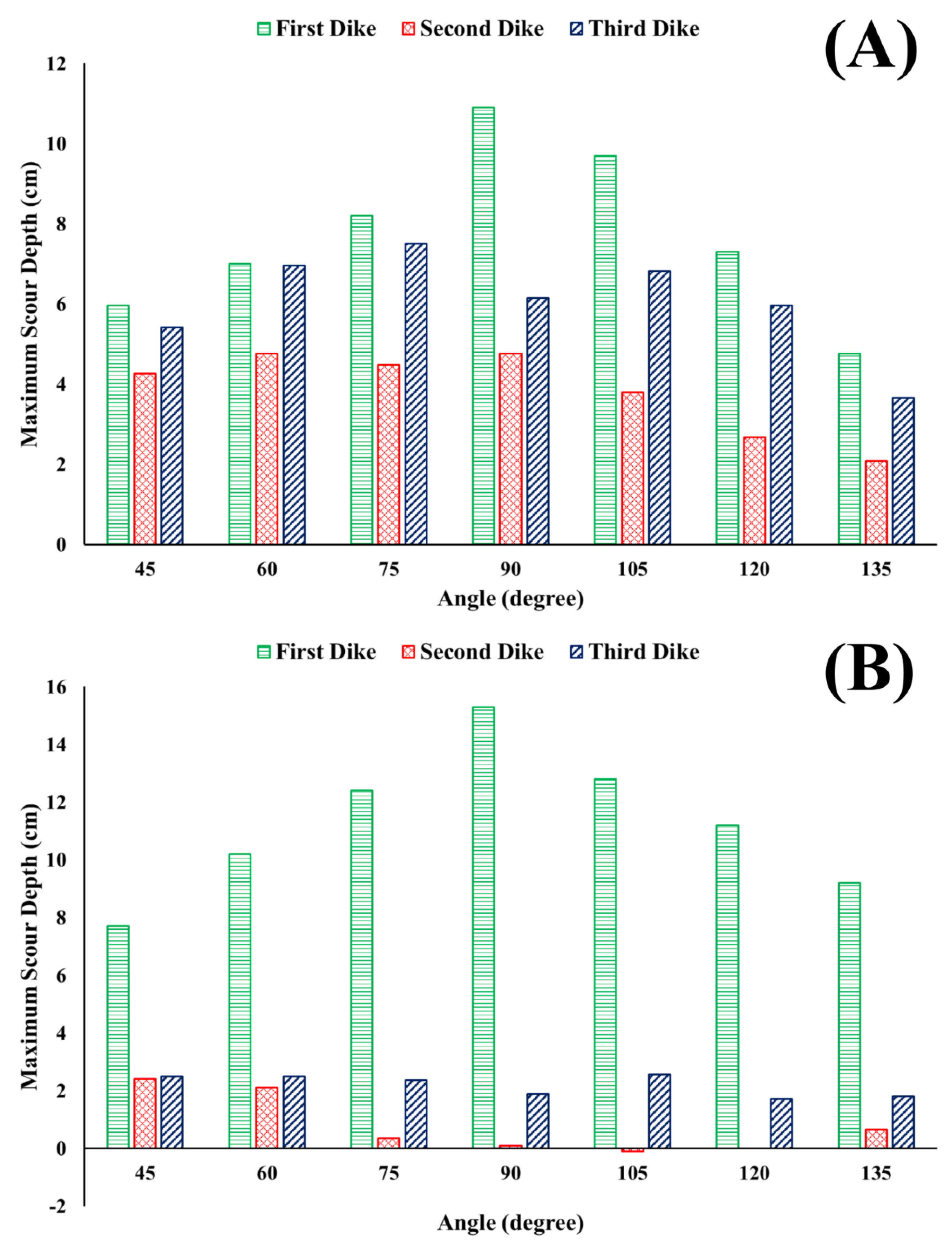
Based on Table 6, Figure 9, and Figure 10, the maximum scour depth increased with an increase in angle until 90°, after which it decreased. Varying the lengths of groynes in an ascending order decreased the scour depth, while a descending order increased the scour depth. Moreover, as was anticipated, the maximum scour depth in simulations 9–15 occurred around the first dike due to the strength of vortices. Scour variation on the second and third groynes are shown in Table 6 and Figure 10. Figure 11 shows the variation of the vortex strength, which decreased due to back flows in farther dikes, (2–7 simulations) while the dike angle increased from 45° to 135°. The strength of these vortices is a function of flow characteristics and shape, and arrangement of the obstacle elements [32,33].

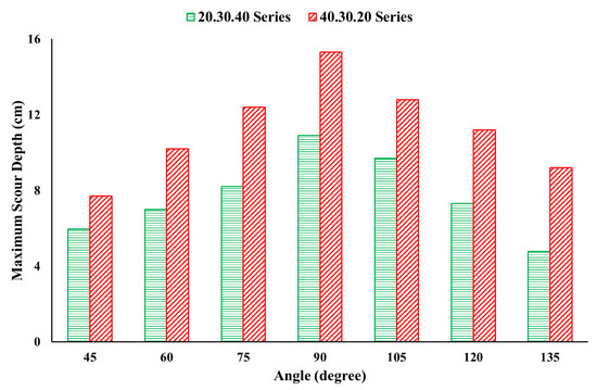
Figure 9. Maximum scour depth in the group of groynes, ascending (green bars), and descending arrangement (red bars).

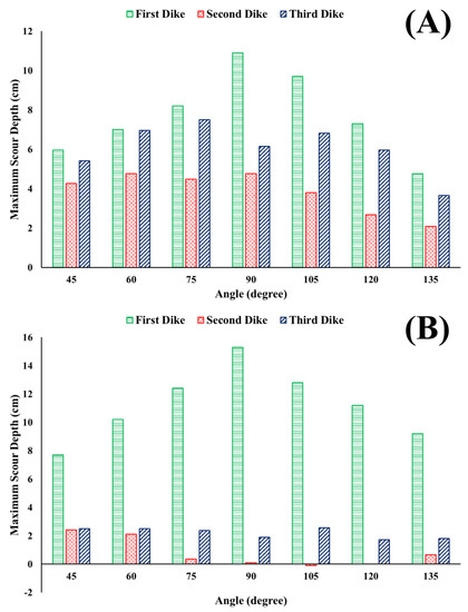
Figure 10. Maximum scour depth under (A) descending and (B) ascending arrangement.

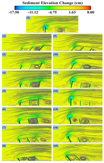
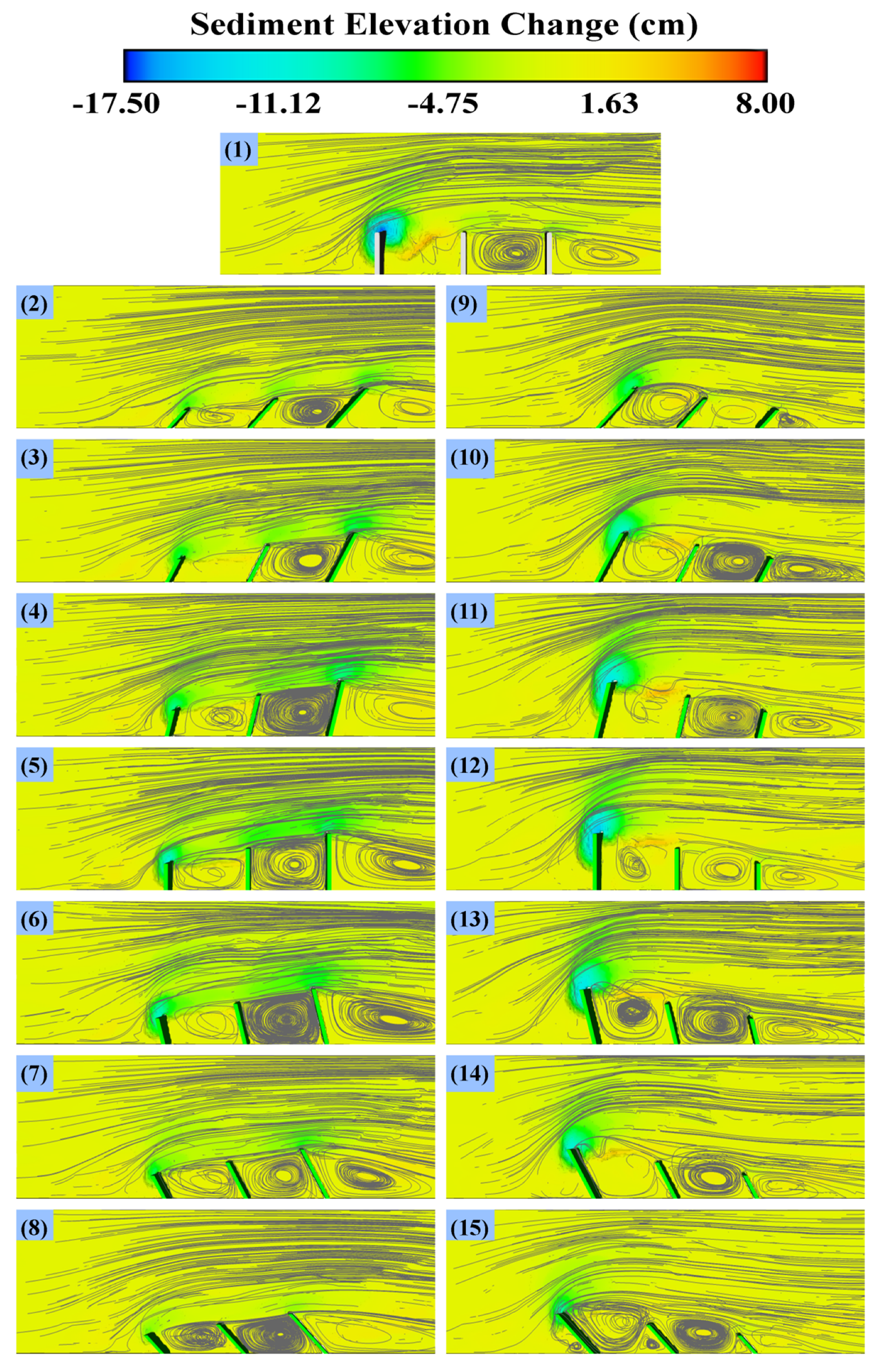
Figure 11. Vortices around groynes under simulations 1–15.

Generally, at an angle of 120° the strength of vortices is minimal compared to other simulations. In simulations 9–15, the length of vortices is weak and shorter. At 75° and 120° angles, the first vortex is not completely established and in these series of simulations, the small and secondary vortices are presented in an orientation of 135°.

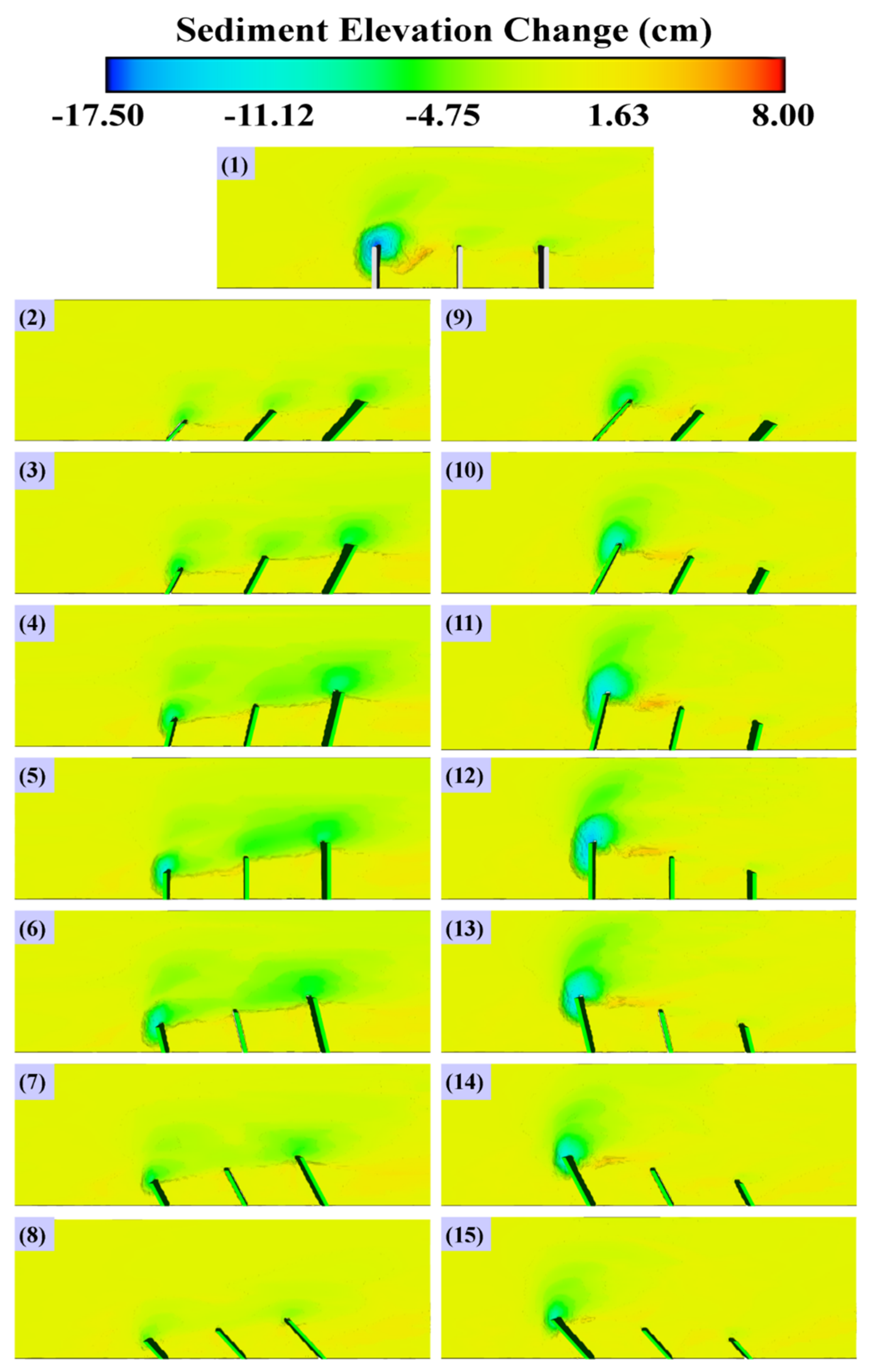
Under simulations 2–7, deposition for all orientations is almost 2 cm. An increment of the groyne angle from 45° to 90° produced a sediment line between the groynes, which is more obvious at 90° (Figure 12). Increasing the angle until 135° removes this sediment line. Besides the deposition between the groynes in all simulations, scour increased beneath the groynes at angles from 45° to 90° to a point where scour holes in the groynes merged.

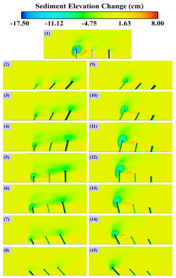
Figure 12. Scour variation under simulations 1–15.

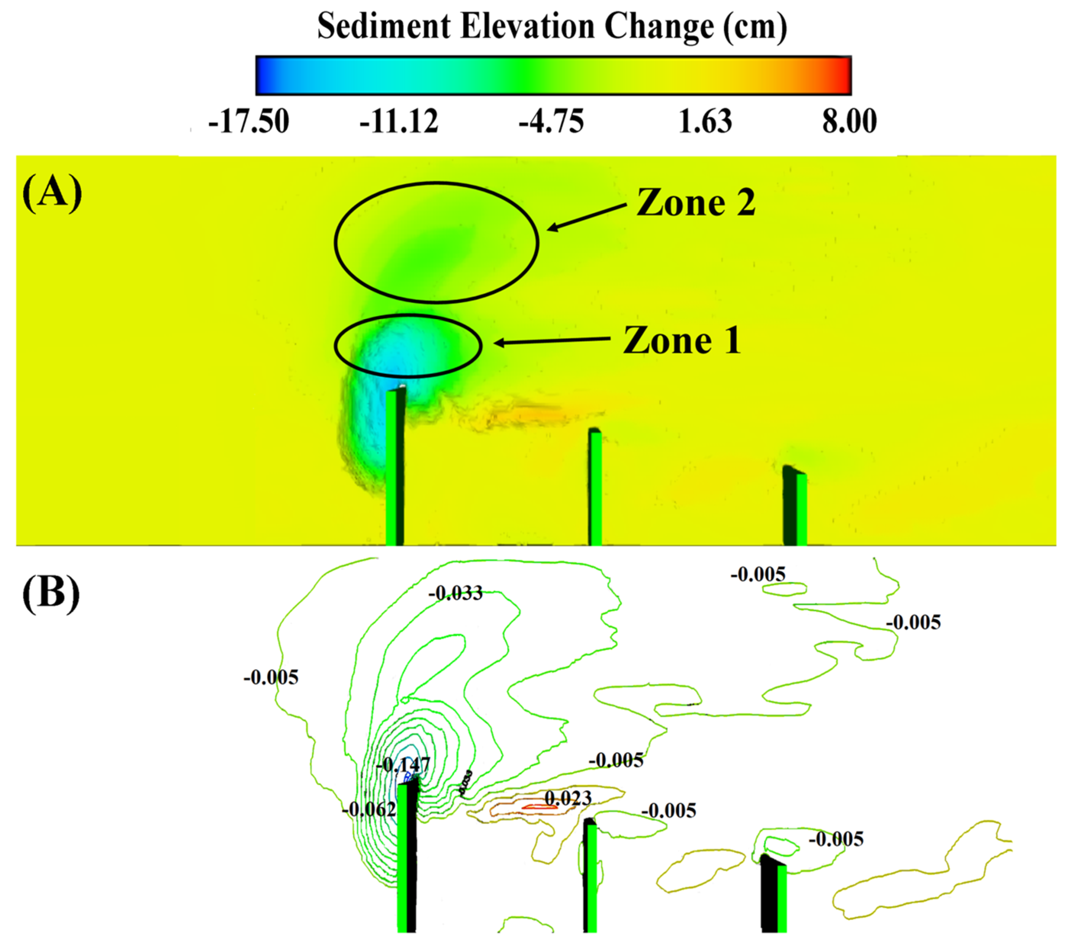
At an angle of 135° these holes are completely separated and the sediment line disappears. In simulations 9–15, the maximum deposition is 3.5 cm, exceeding that of simulations 2–8. Similarly, in Figure 13, the scour hole at zone 1 is greater than in zone 2, due to the strength of vortices in that zone, as discussed in earlier sections.

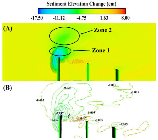
Figure 13. (A) Erosion zone 1 and 2, and (B) erosion and sedimentation contours in simulation 12.

5. Discussion

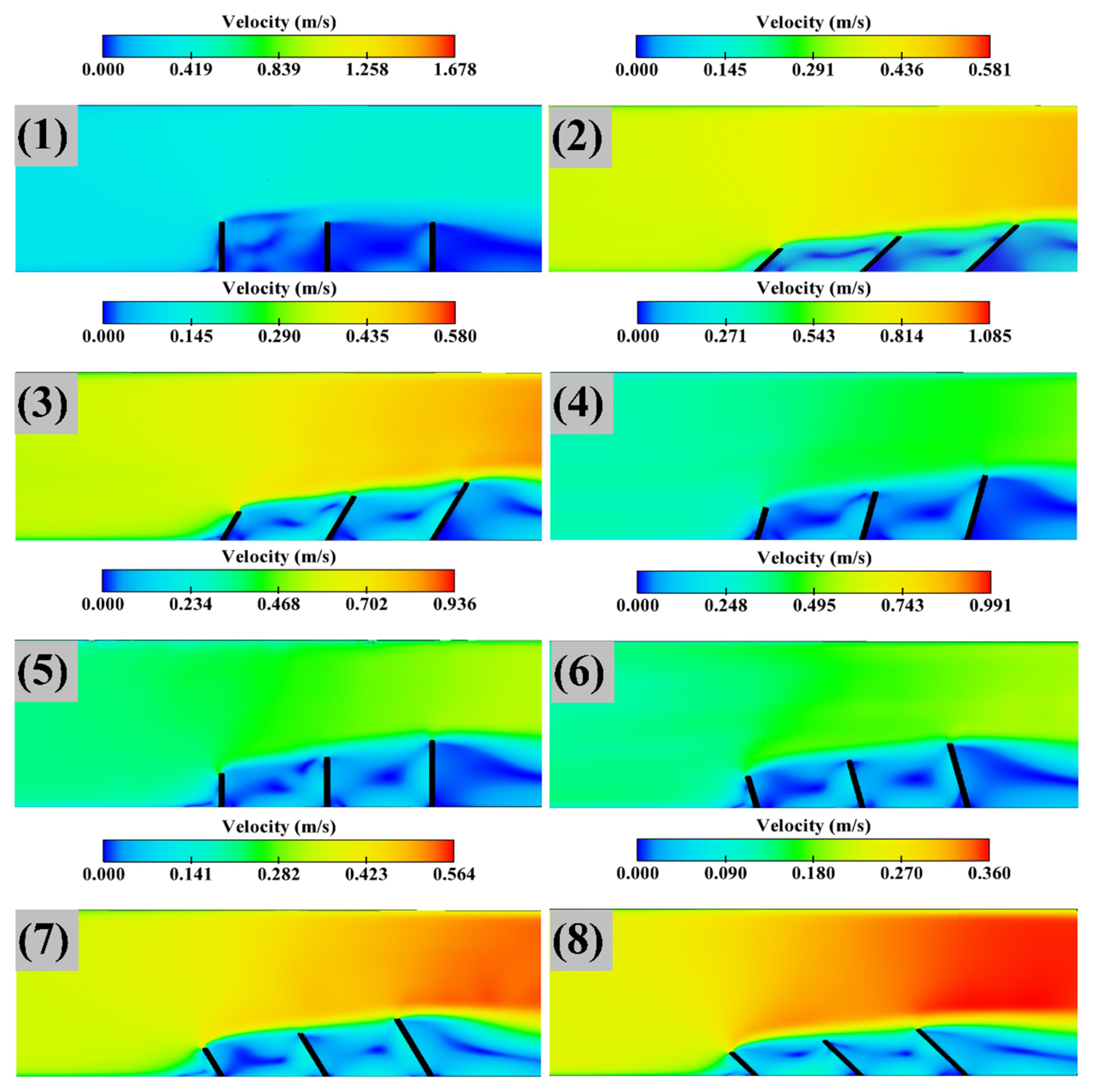
One of the most important dead zones are groyne fields. Dead zones change the velocity profile in a channel and these changes bring profound effects on sedimentation and scour. The flow structure in a dead zone consists of a mixing layer, a primary gyre, and a core region within this gyre. A smaller gyre would exist depending on the aspect ratio of W/L, where W and L are length and distance between them, respectively [12]. The above classification is mainly for a classic groyne or groyne fields, which have the same length, or where a protective groyne exists in the groyne field. Moreover, applying different groyne lengths would yield unique dead zone and flow structure, resulting in special patterns of sedimentation and scour. Illustration is provided for velocity distributions under simulations 1–8 and 9–15, in Figure 14 and Figure 15, respectively.

Figure 14. Velocities in 1–8 simulation.

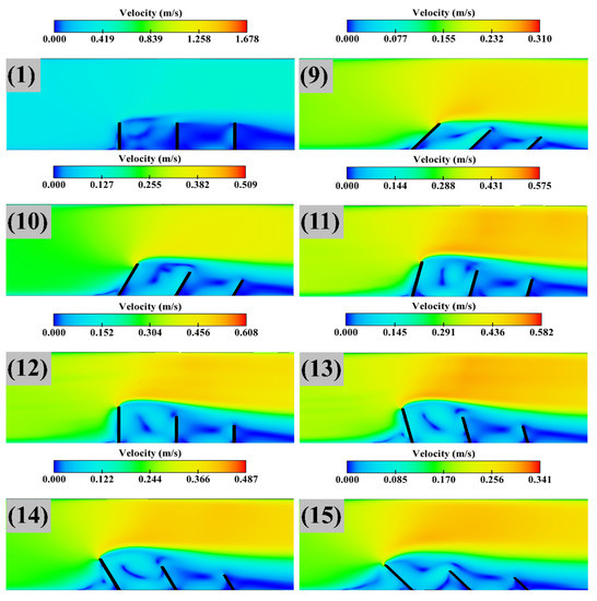
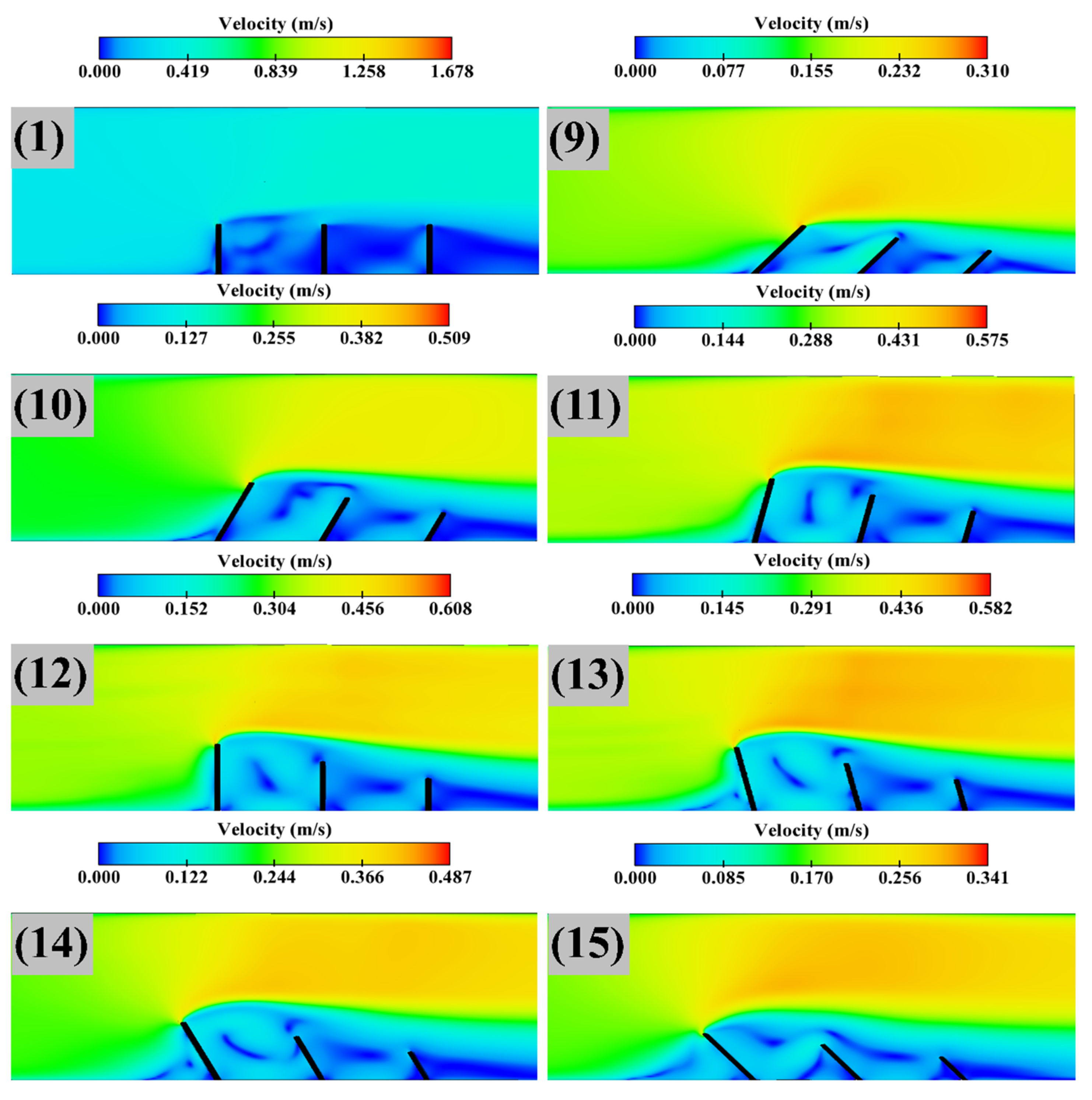
Figure 15. Velocities in simulations 1 and 9–15.

From Figure 14 and Figure 15, the core of the gyres is shown in the regions of low velocity (blue colour). Changing the orientation from 45 to 135 degrees increased the dead zone before the first groyne upstream. This is more obvious in simulations 8 and 15, and the increased dead zone decreased the scour in the order of the orientation angle increase. Under simulations 9–15, the dead zone covers the second and third groynes, and the velocities are lower than the main stream. Hence, the scour becomes smaller as further illustrated by Table 6. On the contrary, in simulations 2–8, the mixing layer would affect the second and third groynes and increase the scour.

Storage time is another important effect of the dead zone, which could be raised by the groyne fields. Dead zones trap large amounts of sediment, which are released back into the main channel after a period. Since the descending simulations had larger dead zones, they trapped more sediment, subsequently increasing the equilibrium times compared to ascending configurations.

Groyne fields with different lengths and orientations have different characteristics compared to classic groyne fields having the same length. One of the main differences between real groynes in the rivers and ideal groynes is that real groynes have 1:3 slopes on their side and nose, whereas ideal groynes are vertical on the side walls [13]. In future studies, the effects of the slopes and the different nose shapes should be investigated. Furthermore, most of the groynes in the rivers are permeable, whereas in this article impermeable groynes were studied. Studying the combined effects of these variables should be sought, i.e., length of groynes, permeability, distance between groynes, orientation, etc.

6. Conclusions

In this paper, a new arrangement of impermeable parallel groynes with non-equal lengths is proposed. The effects of varying the orientation of these groynes and their arrangement on erosion, sedimentation, and flow patterns are discussed. From the numerical assessments, the following conclusions are drawn.

-

When groynes are arranged in an ascending order, more than 50% of scour occurs within 10% of the simulation time, while in a descending order, more than 70% of the scour occurred within a similar time.

-

Simulations with an orientation close to 90° had longer sediment scour equilibrium time.

-

Simulations with an ascending order have larger vortices after the third groyne than those of descending arrangement.

-

Under groynes of 135° with descending arrangement (first groyne: 40 cm; second groyne: 30 cm; third groyne: 20 cm), some small vortices are produced around the groynes.

-

Maximum deposition height when groynes are arranged in an ascending order is higher than in the reverse direction

-

An ascending arrangement produces a sediment line, contrary to a descending orientation

-

Arranging groynes in a descending order could reduce the maximum scour depth by 55%, and ascending arrangement by up to 72%.

References

- Zaid, B.A.; Tait, S. Development of Design Guidelines for Shallow Groynes; Technische Universität Carolo-Wilhelmina zu Braunschweig: Braunschweig, Germany. [CrossRef]
- Vaghefi, M.; Radan, P.; Akbari, M. Flow pattern around attractive, vertical, and repelling t-shaped spur dikes in a mild bend using cfd modeling. Int. J. Civ. Eng. 2018, 1–11. [Google Scholar] [CrossRef]
- Zaid, B.A.; Nardone, P.; Nones, M.; Gerstgraser, C.; Koll, K. Morphodynamic Effects of Stone and Wooden Groynes in a Restored River Reach. In Proceedings of the River Flow 2018-Ninth International Conference on Fluvial Hydraulics, Lyon-Villeurbanne, France, 5–8 September 2018. [Google Scholar]
- Uijttewaal, W.S. Effects of groyne layout on the flow in groyne fields: Laboratory experiments. J. Hydraul. Eng. 2005, 131, 782–791. [Google Scholar] [CrossRef]
- Garde, R.J.; Subramanya, K.S.; Nambudripad, K.D. Study of scour around spur-dikes. J. Hydraul. Div. 1961, 87, 23–37. [Google Scholar]
- Melville, B.W. Local scour at bridge abutments. J. Hydraul. Eng. 1992, 118, 615–631. [Google Scholar] [CrossRef]
- Saneie, M. Experimental Study on Effect of Minor Spur Dike to Reduce Main Spur Dike Scouring; The Food and Agriculture Organization (FAO): Rome, Italy, 2006; pp. 196–200. [Google Scholar]
- Zhang, H.; Nakagawa, H. Characteristics of local flow and bed deformation at impermeable and permeable spur dykes. Annu. J. Hydraul. Eng. 2009, 53, 145–150. [Google Scholar]
- Ghodsian, M.; Vaghefi, M. Experimental study on scour and flow field in a scour hole around a t-shape spur dike in a 90° bend. Int. J. Sediment Res. 2009, 24, 145–158. [Google Scholar] [CrossRef]
- Al-Khateeb, H.M.M.; AL-Thamiry, H.A.K.; Hassan, H.H. Evaluation of local scour development around curved non-submerged impermeable groynes. Int. J. Sci. Technol. Res. 2016, 5, 83–89. [Google Scholar]
- Radan, P.; Vaghefi, M. Flow and scour pattern around submerged and non-submerged t-shaped spur dikes in a 90° bend using the ssiim model. Int. J. River Basin Manag. 2016, 14, 219–232. [Google Scholar] [CrossRef]
- Gualtieri, C. Numerical Simulation of Flow Patterns and Mass Exchange Processes in Dead Zones. In Proceedings of the 4th International Congress on Environmental Modelling and Software, Barcelona, Spain, 6–10 July 2008. [Google Scholar]
- Uijttewaal, W.S.J.; Lehmann, D.; Mazijk, A.V. Exchange processes between a river and its groyne fields: Model experiments. J. Hydraul. Eng. ASCE 2001, 127, 928–936. [Google Scholar] [CrossRef]
- Karami, H.; Basser, H.; Ardeshir, A.; Hosseini, S.H. Verification of numerical study of scour around spur dikes using experimental data. Water Environ. J. 2014, 28, 124–134. [Google Scholar] [CrossRef]
- Acharya, A.; Duan, J.G. Three dimensional simulation of flow field around series of spur dikes. In Proceedings of the World Environmental and Water Resources Congress 2011, Palm Springs, CA, USA, 22–26 May 2011. [Google Scholar]
- Koken, M.; Gogus, M. Effect of spur dike length on the horseshoe vortex system and the bed shear stress distribution. J. Hydraul. Res. 2015, 53, 196–206. [Google Scholar] [CrossRef]
- McCoy, A.; Constantinescu, G.; Weber, L.J. Numerical investigation of flow hydrodynamics in a channel with a series of groynes. J. Hydraul. Eng. 2008, 134, 157–172. [Google Scholar] [CrossRef]
- Yossef, M.F.M.; Vriend, H.J.D. Sediment exchange between a river and its groyne fields: Mobile-bed experiment. J. Hydraul. Eng. ASCE 2010, 136, 610–625. [Google Scholar] [CrossRef]
- Ning, J.; Li, G.D.; Ma, M. 3D Numerical Simulation for Flow and Local Scour Around Spur Dike. In Proceedings of the IAHR World Congress, Kuala Lumpur, Malaysia, 13–18 August 2017. [Google Scholar]
- Abdulmajid, M.; Mohammad, H.; Javad, A. Effect of changes in the hydraulic conditions on the velocity distribution around a l-shaped spur dike at the river bend using flow-3d model. Tech. J. Eng. Appl. Sci. 2013, 3, 1862–1868. [Google Scholar]
- Vaghefi, M.; Ahmadi, A.; Faraji, B. The effect of support structure on flow patterns around t-shape spur dike in 90° bend channel. Arab. J. Sci. Eng. 2015, 40, 1299–1307. [Google Scholar] [CrossRef]
- Giglou, A.N.; McCorquodale, J.A.; Solari, L. Numerical study on the effect of the spur dikes on sedimentation pattern. Ain Shams Eng. J. 2017, 9, 2057–2066. [Google Scholar] [CrossRef]
- Flow Science. Flow-3d User Manual: V10.1; Flow Science, Inc.: Santa Fe, NM, USA, 2012. [Google Scholar]
- Gualtieri, C.; Angeloudis, A.; Bombardelli, F.; Jha, S.; Stoesser, T. On the values for the turbulent schmidt number in environmental flows. Fluids 2017, 2, 17. [Google Scholar] [CrossRef]
- van Rijn, L.C. Mathematical Modelling of Morphological Processes in the Case of Suspended Sediment Transport; Delft University of Technology: Amsterdam, The Netherlands, 1987. [Google Scholar]
- Dodaro, G.; Tafarojnoruz, A.; Sciortino, G.; Adduce, C.; Calomino, F.; Gaudio, R. Modified einstein sediment transport method to simulate the local scour evolution downstream of a rigid bed. J. Hydraul. Eng. 2016, 142, 04016041. [Google Scholar] [CrossRef]
- Dodaro, G.; Tafarojnoruz, A.; Stefanucci, F.; Adduce, C.; Calomino, F.; Gaudio, R.; Sciortino, G. An experimental and numerical study on the spatial and temporal evolution of a scour hole downstream of a rigid bed. In Proceedings of the International Conference on Fluvial Hydraulics, River Flow, Lausanne, Switzerland, 3–5 September 2014; pp. 3–5. [Google Scholar]
- Zhang, H. Study on Flow and Bed Deformation in Channels with Spur Dike; Kyoto University: Kyoto, Japan, 2005. [Google Scholar]
- Gisonni, C.; Hager, W.H.; Unger, J. Spurs in river engineering—A preliminary study. In Proceedings of the 31 IAHR Congress, Seoul, Korea, 11–17 September 2005; pp. 1894–1901. [Google Scholar]
- Chiew, Y.M. Scour protection at bridge piers. J. Hydraul. Eng. 1992, 118, 1260–1269. [Google Scholar] [CrossRef]
- Jahangirzadeh, A.; Basser, H.; Akib, S.; Karami, H.; Naji, S.; Shamshirband, S. Experimental and numerical investigation of the effect of different shapes of collars on the reduction of scour around a single bridge pier. PLoS ONE 2014, 9, e98592. [Google Scholar] [CrossRef] [PubMed]
- Calomino, F.; Tafarojnoruz, A.; Marchis, M.D.; Gaudio, R.; Napoli, E. Experimental and numerical study on the flow field and friction factor in a pressurized corrugated pipe. J. Hydraul. Eng. 2015, 141, 04015027. [Google Scholar] [CrossRef]
- Calomino, F.; Alfonsi, G.; Gaudio, R.; D’Ippolito, A.; Lauria, A.; Tafarojnoruz, A.; Artese, S. Experimental and numerical study of free-surface flows in a corrugated pipe. Water 2018, 10, 638. [Google Scholar] [CrossRef]
© 2019 by the authors. Licensee MDPI, Basel, Switzerland. This article is an open access article distributed under the terms and conditions of the Creative Commons Attribution (CC BY) license (http://creativecommons.org/licenses/by/4.0/).