Abstract
Water quality control remains an important topic of public health since some diseases, such as diarrhea, hepatitis, and cholera, are caused by its consumption. The microbiological quality of drinking water relies mainly on monitoring of Escherichia coli, a bacteria indicator which serves as an early sentinel of potential health hazards for the population. In this study, an electronic nose coupled to a volatile extraction system (was evaluated for the detection of the emitted compounds by E. coli in water samples where its capacity for the quantification of the bacteria was demonstrated). To achieve this purpose, the multisensory system was subjected to control samples for training. Later, it was tested with samples from drinking water treatment plants in two locations of Colombia. For the discrimination and classification of the water samples, the principal component analysis method was implemented obtaining a discrimination variance of 98.03% of the measurements to different concentrations. For the validation of the methodology, the membrane filtration technique was used. In addition, two classification methods were applied to the dataset where a success rate of 90% of classification was obtained using the discriminant function analysis and having a probabilistic neural network coupled to the cross-validation technique (leave-one-out) where a classification rate of 80% was obtained. The application of this methodology achieved an excellent classification of the samples, discriminating the free samples of E. coli from those that contained the bacteria. In the same way, it was observed that the system could correctly estimate the concentration of this bacteria in the samples. The proposed method in this study has a high potential to be applied in the determination of E. coli in drinking water since, in addition for estimating concentration ranges and having the necessary sensitivity, it significantly reduces the time of analysis compared to traditional methods.
1. Introduction
Water quality coming from drinking-water treatment plants (DWTPs) continues being a worldwide problem, especially in developing countries [1]. Deficiencies in water sanitation cause a serious impact on the population, as it affects health causing a large number of diseases caused by microorganisms [2]. Waterborne disease is a global problem. According to the World Health Organization (WHO), each year 3.4 million people, mostly children, die from water-related diseases [3]. This organization reported that more than 2.6 billion people cannot access to clean water of which is responsible for about 2.2 million deaths annually whereas 1.4 million were children [4]. Although water-associated diseases in developing countries are prevalent, they are also a serious challenge in developed countries [5].
The microbiological quality control of water for human consumption requires a simple and reliable assessment of the presence of pathogens [2,6]. One of the most abundant bacteria associated with the sanitary risk of water is Escherichia coli [6]. The presence of E. coli indicates that there is a high risk of the incidence of other bacteria and viruses of faecal origin in which many of them are pathogenic. For this reason, E. coli is used as an indicator organism to identify water samples that may contain unacceptable levels of faecal contamination [7,8]. That is why E. coli has become a quality parameter for the creation of regulations or standards where the maximum admissible limits of this bacterial indicator are established. For drinking water, the parameter is used to evaluate the efficiency of the disinfection process. In such case, the necessary corrective measures must be taken in order to offer water of optimum quality for human consumption and complying with the requirements of the regulations [8].
Nowadays, for the E. coli detection in water, standardized and regulated conventional techniques are used. These techniques are based on the cultivation of bacteria such as fermentation of multiple tubes, membrane filtration, and methods that use defined substrates, among others [9,10,11]. Membrane filtration is perhaps the most used method for the routine enumeration of coliforms in drinking water due to its practicality. In spite of that, all these techniques present important limitations. The most important is the prolonged incubation time for the final detection of E. coli, requiring at least 24–28 h [12,13]. It is worrisome that a positive result of this pathogen is detected when the water has already reached the distribution system of the different houses of the population being too late to generate a suitable response. Furthermore, some conventional methods are questioned for their sensitivity to the interference of microorganisms or antagonistic substances and the deficient detection of viable but non-cultivable bacteria. The above can lead to false negatives of E. coli in water samples [10]. In other cases, including molecular techniques, cannot differentiate between viable and non-viable bacteria; so, this tends to overestimate the contamination of the sample. Additionally, these are expensive methods that require complex equipment, specific reagents, and lack the standardization process to obtain protocols for the sample’s analysis [14]. These limitations can place public health at risk. This is why many research studies have focused on the development of fast and accurate methods for E. coli detection in drinking water [15,16,17,18,19,20].
The use of smell detection technology, well known such as the electronic nose has been investigated as an alternative instrumental method of great utility for the specific analysis, identification and recognition of volatile organic compounds (VOCs) emanated by bacteria [21,22,23,24,25,26,27]. The electronic noses (e-noses) are composed by a set of chemical gas sensors with overlapping sensitivities whereas each one responds differently to the composites emanating from the sample, obtaining a characteristic smell-print to be analysed.
In the samples collection, it requires that each sample in gas phase contains composites of the bacterial species in order to be measured using a sensor array with good sensitivity and selectivity. The sensor responses should be represented regarding the specific components of the bacterial species that makes up the sample as well as improving the quality of classification and robustness in the measurement. Some references of electronic noses applied in water quality control are listed below [28,29,30,31,32,33,34,35,36]. A way to increase the sensitivity and selectivity is to incorporate different sampler methods. For this, there are some techniques such as Solid Phase Microextraction (SPME) that consists of two steps: extraction and desorption of the analyte. Although this method is very effective, it depends on certain sampling parameters such as the type of fibre coating (this means that VOCs vary according to fibre type), extraction time, equilibrium time, extraction temperature, and desorption. Additionally, there are dynamic and static headspace methods. The first one consists of submitting a sample at a certain temperature by means of an inert gas [37]. The volatile compounds are subsequently retained in an adsorbent trap and then they are injected for its separation through gas chromatography.
Furthermore, the static headspace method is very simple to use and it is inexpensive. That is why in this research study a static headspace sampler system “home-made” was developed. This mechanism consisted of introducing the sample in a closed vial through a septum applying a determined temperature with the objective to extract an aliquot of the vapour fraction with a syringe for gaseous samples [38] that was injected in the gas-chromatographic and mass-spectrometry (GC-MS) [39,40].
In this study, a multisensory system was tested using samples collected from Pamplona and Toledo DWTPs located in the north of Santander department (Colombia). The tests were carried out in a parallel way. As a validation technique, the membrane filtration (MF) method was used to detect the E. coli concentration in water. Finally, the results obtained by means of both techniques were compared.
2. Materials and Methods
Figure 1 illustrates the general measurement and classification system: (1) sample preparation and suitability on the vials, (2) headspace sampler (Head sampler), (3) sensory perception system, and (4) a data acquisition card connected to the sensor chamber and the computer. The individual components are described below.
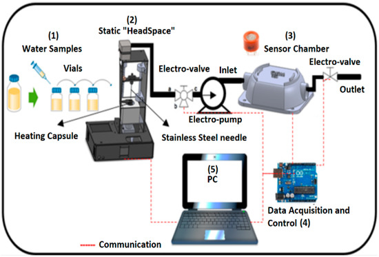
Figure 1.
Scheme of the measurement system.
2.1. Bacterial Strain and Control Samples Preparation
In this study, the bacterial strain Escherichia coli (ATCC 25922) was used. It was preserved in the microbiology collection centre of the University of Pamplona.
Initially 10 mL of a bacterial suspension was prepared on sterile water at a concentration of 3 × 10⁸ CFU/mL. For this, isolated colonies of E. coli that were grown in nutritive agar at 35 ± 2 °C for 18–24 h were taken.
This bacterial suspension was diluted to obtain the final concentrations: 1 × 10⁷, 1 × 10⁵, 1 × 10³, 1 × 10², 1 × 101, 1 × 100, 1 × 10⁻¹, and 1 × 10⁻² CFU/mL (see Figure 2) [41]. The choice of this final concentration (1 × 10⁻² CFU/mL) was due to the fact that the local regulations establish that there should not be presence of E. coli in 100 mL of sample. From each of the Erlenmeyer, 20 mL were taken in a vial to be analysed by the e-nose. This analysis was repeated ten times for each concentration. The negative control was prepared by sterilizing drinking water (121 °C/15 psi/15 min). As was mentioned above, the aim of this study was to verify the capability of the e-nose to discriminate different concentration of E. coli. The bacterial classification approach can be seen in the first study made by the authors of this research [42].
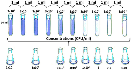
Figure 2.
Procedure carried out for the dilution of the control of E. coli.
2.2. Sampling and Treatment of Samples
As was mentioned above, this study was developed in the municipalities of Toledo and Pamplona located in North of Santander (Colombia). The samples were taken from both DWTPs of these municipalities. In order to make the comparison between the conventional methodology and the proposed method, several sampling points were selected in each treatment plant. Entrance of the plant, after the sedimentation and the outlet from the plant and water taken from the tap of a house were the sampling points for the Toledo plant. In Pamplona, the sampling points were the same, except the outlet from the plant.
The samples were analysed in parallel way by a Volatiles Extraction System (VES) coupled to the e-nose and the MF conventional method. These methodologies were tested to determine the E. coli concentration in the samples collected. When the analysis by VES coupled to the e-nose was carried out, the control samples were prepared as indicated in Section 2.1 (see above). The sterilized water from the respective treatment plant was used and the samples from the treatment plants were analysed together with the control samples. Furthermore, the membrane filtration method was performed as follows: a sample of 100 mL of water was passed through a 47-mm diameter cellulose sterile filter (0.45-μm, Millipore, Burlington, MA, USA) and transferred to a plate on a selective medium to allow the growth of bacteria for 24 h at 35 ± 2 °C. The selective medium used was Chromocult® Coliform Agar, (Merck, Darmstadt, Germany) [15].
Figure 3 illustrates the stages that were part of the drinking-water treatment plants.
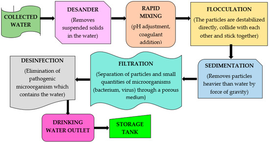
Figure 3.
Diagram of the unit operations that makes up the drinking-water treatment plant.
2.3. Generation of HeadSpace of the Samples
In this research, the VES technique for the extraction and concentration of composites emanating from the sterile water samples was applied and the water with E. coli samples were collected from the different points of the treatment plants.
Since there was no equipment to perform this procedure, a “home-made” volatile extraction system was constructed, taking into account the combination of incubation time and temperature to increase the concentration of volatile analytes in order to reach a balance before to be detected with the multisensory system (see Figure 4).
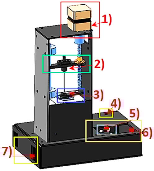
Figure 4.
Design of the volatiles extraction system (VES).
The operation of the VES was based on the temperature control of a heating capsule (3) and the operation of a stepper motor (1) for automatic control of the injector (2). The temperature of the heating capsule was regulated by a proportional, integral, and derivative (PID) controller of discrete-type implemented in a low-cost data acquisition card used in an embedded way (Arduino Mega, 2560). This flexible and easy process began when the sample was prepared. A 20 mL vial was sealed by a septum which was placed inside the capsule with the objective to apply and maintain the temperature at 50 °C and generate the volatile components to a vapour phase (upper space of the road known as “Headspace”). Through a user graphical interface (5, 6) (liquid crystal display (LCD)) the incubation time necessary to generate the volatilization of the compounds and temperature of the sample in a range of 0 to 110 °C was defined.
All components were energized by using two power supplies (4, 7) of 12 VDC and 24 VDC, respectively. Table 1 shows the parameters used to generate the headspace of the samples.

Table 1.
Parameters used in the experiments of Escherichia coli discrimination.
It should be noted that 10 mL of sample volume were used in this study since the electronic nose and the VES system (using vials of 20 mL) were conditioned to detect less amount of the sample. For this reason, although the international regulation recommends to evaluate the E. coli to 100 mL of volume, in this case 10 mL it was enough to test the sensibility and selectivity of the proposed system. It allowed to avoid the saturation of the sensors in order to improve the recovery time. Once the warm-up-time was reached (around 15 min) it was possible to make measurements in rapid way since all vials could also be heated in just a few minute (five minutes).
Once the desired temperature was reached, the stepper motor was activated. It moved down to a stainless-steel syringe in order to extract the volatile compounds from the vial. In this step, an electro-pump and a three-way solenoid valve were activated for a specific time that allowed all the generated volatile compounds to be drawn into the sensor chamber inlet.
2.4. Generation of Headspace.
A chamber composed by 16 metal oxide gas sensors (Taguchis from the Figaro company, Arlington Heights, IL, USA) was coupled to the headspace system. Table 2 describes the gas sensors implemented in this study. It is important to clarify that five duplicate-sensors (i.e., TGS 826, TGS 831, TGS 821, TGS 842, and TGS 880) were placed inside of the sensor chamber since they showed good sensitivity and selectivity. Although these duplicate-sensors belonged to the same model, their responses were different. Therefore, useful and reliable information in the dataset were obtained in order to achieve the expected results. These commercial gas sensors are manufactured by means of a resistive sensing material and its responses will never be equal to each other.
Table 2.
List of sensors that make up the sensor matrix of the e-nose.
The system was composed of three stages, such as: (1) the sampling stage (e.g., static headspace) which was replaced by the VES with flow control, (2) a sensor array and (3) a computational system. Table 3 shows the time parameters defined in the e-nose system.
Table 3.
Parameters.
2.5. Generation of Headspace of the Samples
Once the signals were acquired, a data pre-processing stage was applied to the samples [43]. This stage was applied since the outputs of the sensors could present drifts and redundant information that must be treated before obtaining the responses of the e-nose system. The signals obtained by the sensor matrix were adjusted. Furthermore, several static parameters were extracted from the sensor signals and data normalization.
It was considered the maximum conductance parameter (∆G = Gmax − Gmin) to extract the relevant information of each sensor where Gmax corresponded the maximum response value of the sensor to the reaction with the compound and Gmin was the baseline and/or the value of the steady state of the sensor. Once the parameters of the sensors were extracted, it was necessary to scale the information in order to apply the pattern recognition algorithms. There were several types of scaling: linear, logarithmic, variables or measures. It should be noted that for this research, four types of standardization methods were tested: auto-scaling, centring, and normalization by column and by matrix. All measurements were analysed using multivariate statistics techniques such as PCA and DFA. On the other hand, a PNN network was applied to the dataset. A short description of each method is shown below.
Principal Component Analysis (PCA): PCA is a multivariate analysis method that is widely useful in feature reduction, data compression, variable selection, and sometimes used for noise reduction. This statistical powerful procedure for data analysis was selected in this application since it is an effective linear unsupervised method to extract the most relevant information and project data from several sensors to a two-dimensional plane using scores plot. Therefore, it is possible to discriminate properly a data set, finding the directions of maximal variance. PCA returned a new basis which is a linear combination of the original basis [44]. Each vector (orthogonal) has an amount of variance in the data set with a different degree of importance. The scalar product of the orthogonal vectors gives the value of the principal component.
Discriminant Function Analysis (DFA): It is a supervised method unlike PCA analysis, which it is able to reduce the dimensionality and classify a dataset while preserving as much of the class discriminatory information as possible. DFA maximizes the ratio of between class variance to the within-class variance in any data set, further it provides maximal discrimination and usually a number of two latent variables (i.e., first two canonical variables) of a linear combination of independent variables can be selected for classification [45].
Probabilistic Neural Network (PNN): This method was applied in this study to classify the data set, it provides a solution to measure classification problems. It is a biologically-inspired process that works similar to the human brain and that uses a training set to generate distribution functions (i.e., Gaussian distribution) with different layers. The algorithm requires less computational cost and high training speed compared to other methods [46].
3. Results
To use the PCA statistical technique, the static parameter ∆G was applied. Afterwards, the matrix normalization method was obtained and applied to be used with the PCA analysis making all the sensors with equal weight. At the end of this procedure, a statistical PCA model was created in order to project a new group of measurements into the plot. Figure 5 presents the first analysis of the main components of sterile water samples and the contaminated samples with E. coli at different concentrations. This experiment was done in order to verify the performance of the e-nose to distinguish the different categories. For data processing, a number of representative information was acquired (10 measurements for each category) by means of the first two principal components (PC1 and PC2). It is very important to clarify that those 10 measurements were acquired with the VES and e-nose system, but there were some outliers due to the experimental problems (e.g., power supply fluctuations on temperature control of VES). Therefore, two and three measurements were removed from dataset.
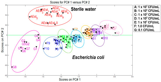
Figure 5.
PCA plot of sterile water and different concentrations of E. coli.
According to the plot, good discrimination between two study groups (sterile water and water inoculated with E. coli) was obtained. The separation of two categories (i.e., sterile water and E. coli) is clearly observed leaving in the upper part the free samples of any contaminant and in the lower part the contaminants samples with E. coli at different concentrations. The discrimination of the seven groups of different concentrations was clearly determined by obtaining a total variance of 98.03%.
In the same way to PCA, through analysing the results obtained with DFA (see Figure 6) there were some overlapping in some samples, especially at low concentrations. Therefore, the clusters corresponding to the categories under study could be clearly identified. By means of the first two factors a DFA analysis of 91.5% was obtained, getting a good response to the functioning of the system.
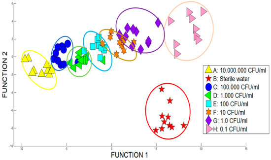
Figure 6.
DFA chart of sterile water and different concentrations of E. coli.
3.1. Comparison between the Samples Collected in the Treatment Plant
Table 4 summarizes the results obtained with the normalization and data processing methods from two plants, where P1 corresponds to the Pamplona plant and P2 to the Toledo plant. It can be seen that the best result for the discrimination of the measurements was obtained using the matrix normalization method and applying the PCA and DFA pattern recognition methods. Likewise, applying the PNN with the cross-validation technique (leave-one-out), a better success rate was obtained for the measurements classification using the matrix normalization method.
Table 4.
Results of the methods of normalization and data processing.
3.1.1. Pamplona Plant
Making the PCA plot, the data of the control samples (A, C–E, G, I) and the water samples from the water treatment plant (B, F, and H) were used. The comparison was made with the purpose of evaluating the capacity of the system to discriminate and separate the samples (see Figure 8). A good cluster discrimination could be observed between different categories by using PCA (80.4% of variance). Tap water samples (B) were discriminated close to the sterile water (A), indicating the bacteria absent. On the other hand, sediment (F) and input (H) water samples were differentiated with the measurements of inoculated concentrations by E. coli (see Figure 7).
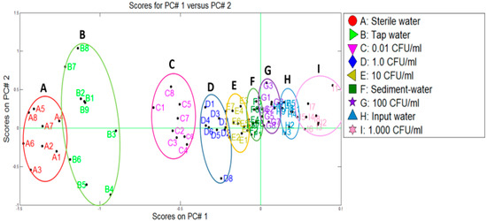
Figure 7.
PCA plot of the set of measurements of training samples and samples taken of Empopamplona plant.
3.1.2. Toledo Plant
In a similar way to the Pamplona plant, the data from the control samples (A, D–F, H, J) and water samples from the Toledo treatment plant (B, C, G, I) were used. Figure 8 depicts the two categories that were discriminated using PCA (uncontaminated water and the contaminated water with E. coli at different co-concentrations) where a variance of 90.2% was reached from the first two components. We could observe that Toledo plant presented a similar behaviour to the Pamplona one but in this case the samples of the outlet of the plant were added and grouped on the left part of the PCA plot with the sterile water samples and tap water samples, indicating that there was not E. coli presence. On the other hand, the samples of the settler and the inlet water were grouped in different concentration ranges on the right part of the PCA plot.
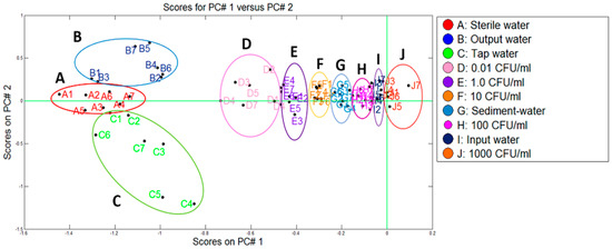
Figure 8.
PCA plot of the set of measurements of training samples from Toledo plant.
For the E. coli quantification of the collected samples from two plants, the membrane filtration technique was used. It was applied in parallel way with the VES and e-nose system. The E. coli counted in plates were reported in colony, forming units per millilitre (CFU/mL) which are listed in Table 5, where the P1 (Pamplona plant) data ranged from 0 to 345 CFU/mL and P2 (Toledo plant) between 0 to 125 CFU/mL.
Table 5.
Comparison of the results obtained by the two techniques.
It is important to note that MF values as well as e-nose ranges were matched in order to verify the amount of CFU/mL obtained in the sample. It was concluded that with more tests the e-nose might be able to estimate the number of colonies counted by MF.
4. Discussion
To evaluate the water quality, the microbiological requirements demanded by the Colombian regulations were taken into account. From a microbiological point of view, in both treatment plants, the population of E. coli presented similar behaviour. The water from the entrance of the plants showed an amount of E. coli greater than 100 CFU/mL. After the settler, the amount of E. coli was reduced between 5 and 10 times and, finally, the water of the outlet of the plant did not present viable cells of E. coli in 100 mL of water as required by the norm. It was also observed that the distribution system was not a contamination source by this bacterium because the samples of the taps in the houses presented negative results for E. coli.
On the other hand, from the results obtained by the two methodologies tested, it could be deduced that in both treatment plants, the samples of outlet water and tap water were grouped in the category of samples free of E. coli (left part of Figure 7 and Figure 8), that were located next to the reference sample of sterile water and matching with the obtained concentration by the membrane filtration method, <0.01 CFU/mL for both cases. Likewise, it was possible to discriminate the contaminated samples from the plants in ranges of concentrations of 100 to 1000 CFU/mL. This is the case of the samples of water from the entrance of the plants, for which the membrane filtration method generated counts of 345 CFU/mL and 145 CFU/mL, for plants P1 and P2, respectively. In the same way, through the response of the e-nose, concentrations between 10 and 100 CFU/mL were determined for the samples from the settler. When compared to the microbiological method, a total coincidence was observed, since in the P1 the count was of 31 CFU/mL and in the P2 of 26 CFU/mL. These results indicated an excellent correlation between the data obtained by both methodologies.
According to what is observed in the two plants, it can be seen that the proposed method has a degree of repeatability and reproducibility in the measurements, since the same procedure was applied for the two DWTP’s, the same operating conditions and the results achieved follow the same behaviours. In addition, the two methods implemented showed similarity in terms of detection capacity, identification and an approximation in concentration ranges.
Figure 9 shows the response time comparison among the two methods. By means the conventional method of membrane filtration (a) and their different stages, such as the mixture preparation process, followed by the detection and confirmation stages of the bacteria. Results were obtained around 24–28 h approximately. On the other hand, the proposed method (b) using the different electronic nose subsystems such as: gas sensors, feature extraction technique, and data discrimination/classification methods coupled to the VES system performed on this study. Results were obtained in 30 min. Therefore, it was possible to reduce the response time for concentration detection of E. coli in drinking water using the proposed method. It should be noted that to train the system was necessary to create a model (PCA or DFA) by using 10 measurements for each category (Total: 80 measurements). Therefore, this procedure took 15 h approximately. Afterwards, the analysis was done in just 30 min.
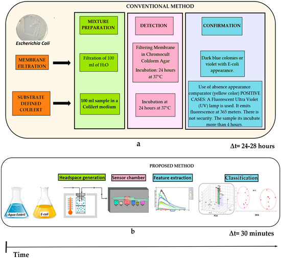
Figure 9.
Response time comparison: (a) Conventional method and (b) proposed method.
The procedure of the dilutions carried out also allowed us to make an approximation of the sensitivity for the proposed method. In the first instance, as can be seen in Figure 5 and Figure 6, regardless of whether the data were treated by PCA or DFA, our methodology generated a good discrimination between all tested concentrations, being able to discriminate very well between sterile water and water with concentrations of 1 and 0.1 CFU/mL of E. coli. Furthermore, these results were obtained in lower concentrations (i.e., 0.01 CFU/mL of E. coli). As mentioned in materials and methods (Section 2.1), in the election of this final concentration, the limit required by the regulations was taken into account. Thus, when testing this limit concentration, we observed how the e-nose, certainly, distinguished between water samples with concentrations of up to 0.01 CFU/mL and separated them from water samples free of the bacteria (see Figure 8 and Figure 9). These results showed the ability of the e-nose to discriminate samples with very low concentrations of E. coli, which indicates that the sensitivity of the proposed methodology is optimal for the analysis of this type of samples, especially from the point of view of public health.
In this study the e-nose was able to detect E. coli concentrations by using a sample volume of 10 mL due to the experimental design of the sensing system. The measurement protocol and tests performed with the VES coupled to e-nose were conducted taking into account others studies that used headspace sampler techniques such as gas sensors and others methods (GC-MS) [17,18]. In these experiments, different bacterial suspensions of 5 mL to 10 mL were transferred into standard 20 mL headspace vials. Regarding to e-nose, it was an easily-operated tool with a quickly-response and portable tool for bacterial samples detection. However, this methodology has some limitations since it is not able to detect VOCs in a specified way due that e-nose it is a “all or nothing” process in comparison with MF, which can detect bacterial colonies by count.
As a future work, it would be important to use conventional methods such as gas GC-MS in order to evaluate and validate the identification and classification of E. coli concentration in DWTP’s, by comparing with the MF technique and the proposed method.
5. Conclusions
As was mentioned, although the international regulation recommends to evaluate the E. coli to 100 mL of volume from drinking water samples for the determination of this bacteria, the results in the proposed methodology showed that the e-nose had a good sensitivity to detect the bacteria at the concentrations required by the standard. It should be noted, however, that the volume requirement was used to avoid false negatives, since the membrane filtration method was based on the cultivation of viable cells that were retained on the membrane surface. For its part, the proposed technique was able to analyse the gas phase generated by the sample, so it is not a crop-dependent procedure. With the obtained results we can infer that the potential use of the e-nose is to detect E. coli at low concentrations.
The results demonstrated that the proposed methodology allowed an effective evaluation between the contaminated samples and control samples. It is observed an excellent discrimination of the categories for the samples obtained from both drinking water treatment plants. The negative samples for E. coli were clustered together with the sterile water, while the test samples were located between concentration ranges that allowed to estimate the concentration of E. coli in water.
The system VES coupled to the e-nose allowed to discriminate sterile water samples from contaminated samples with E. coli at different concentrations. In the same way, it was possible to classify each of the seven groups belonging to the different concentrations (from 1 × 10⁷ to 0.01 CFU/mL) obtaining a total variance captured of 98.03% using the PCA technique. Additionally, the system demonstrated sufficient sensitivity to detect and discriminate contaminated samples with concentrations of 0.01 CFU/mL of E. coli from sterile samples. Moreover, this tool could be used for other purposes (e.g., spoilage of fruits, early detection of microbial contamination in processed food, screening of fungal species, pesticides detection, among others) in developing and developed countries.
By comparing the concentration ranges estimated by the VES coupled to the e-nose, with the results of the quantification of E. coli by using the membrane filtration method, the relation was observed through PCA statistical analysis. These results supported the capacity and certainty of the proposed method to estimate the concentration of this bacteria in drinking water samples.
Taking into account that the main disadvantage of conventional methods is the time it takes to obtain results due to the long periods of incubation, it can be said that the biggest advantage of the tested methodology was the rapid response time (i.e., 28 h with MF and 30 min with e-nose) to obtain results because once the system was trained, the analysis could be done in a few minutes. Likewise, the proposed method could save the operation costs as it does not require the purchase or preparation of culture media and everything related to conventional analysis.
The system VES coupled to the e-nose could be a promising analysis tool to be applied for bacterial detection due to its speed and ease of use.
Author Contributions
J.C. wrote and proofread the manuscript, C.D. arranged the materials and wrote the manuscript with provided technical feedback, and R.O performed the different microbiological analysis of contaminated water with E. coli and provided technical feedback.
Funding
This research was funded by H2020-MSCA-RISE-2017 “bTB-Test” project, grant number 777832.
Acknowledgments
The authors of the work acknowledge the collaboration and contribution in this study to the Pamplona and Toledo drinking-water treatment plants and H2020-MSCA-RISE-2017 “bTB-Test” project, of the European Commission.
Conflicts of Interest
The authors declare no conflict of interest.
References
- Bain, R.; Cronk, R.; Wright, J.; Yang, H.; Slaymaker, T.; Bartram, J. Fecal Contamination of Drinking Water in Low and Middle Income Countries: A Systematic Review and Meta-Analysis. PLoS Med. 2014, 11, e1001644. [Google Scholar] [CrossRef]
- Cabral, J.P. Water microbiology. Bacterial pathogens and water. Int. J. Environ. Res. Heal. 2010, 7, 3657–3703. [Google Scholar] [CrossRef] [PubMed]
- World Health Organization. Drinking-Water. Available online: https://www.who.int/news-room/fact-sheets/detail/drinking-water (accessed on 6 February 2019).
- Castillo, F.R.; Muro, A.L.; Jacques, M.; Garneau, P.; González, F.A.; Harel, J.; Barrera, A.G. Waterborne Pathogens: Detection Methods and Challenges. Pathogens 2015, 4, 307–334. [Google Scholar] [CrossRef] [PubMed]
- Arnone, R.D.; Walling, J.P. Waterborne pathogens in urban watersheds. J. Heal. 2007, 5, 149–162. [Google Scholar] [CrossRef]
- Levy, K.; Nelson, K.L.; Hubbard, A.; Eisenberg, J.N. Rethinking indicators of microbial drinking water quality for health studies in tropical developing countries: Case study in northern coastal Ecuador. Am. J. Trop. Med. Hygien 2012, 86, 499–507. [Google Scholar] [CrossRef]
- Edberg, S.C.; Rice, E.W.; Karlin, R.J.; Allen, M.J. Escherichia coli: The best biological drinking water indicator for public health protection. J. Appl. Microbiol. 2000, 88, 106S–116S. [Google Scholar] [CrossRef]
- Odonkor, S.T.; Ampofo, J.K. Escherichia coli as an indicator of bacteriological quality of water: An overview. Microbiol. Res. 2013, 4, 2. [Google Scholar] [CrossRef]
- Guidelines for the Prevention and Control of Infection from Water Systems in Healthcare Facilities Health Protection Surveillance Centre Prepared by the Prevention and Control of Infection from Water Systems in Healthcare Facilities Sub-Committee of the HPSC Scientific Advisory Committee. 2015. Available online: http://www.hpsc.ie/abouthpsc/scientificcommittees/publications/Water%20systems%20in%20healthcre%20facilities%20FINAL%20amended%20May%202017.pdf (accessed on 7 February 2019).
- Deshmukh, R.A.; Joshi, K.; Bhand, S.; Roy, U. Recent developments in detection and enumeration of waterborne bacteria: A retrospective minireview. MicrobiologyOpen 2016, 5, 901–922. [Google Scholar] [CrossRef]
- Rompré, A.; Servais, P.; Baudart, J.; De-Roubin, M.R.; Laurent, P. Detection and enumeration of coliforms in drinking water: Current methods and emerging approaches. J. Microbiol. Methods 2002, 49, 31–54. [Google Scholar] [CrossRef]
- Niemi, R.M.; Heikkilä, M.P.; Lahti, K.; Kalso, S. Comparison of methods for determining the numbers and species distribution of coliform bacteria in well water samples. J. Appl. Microbiol. 2001, 90, 850–858. [Google Scholar] [CrossRef]
- Mendes, D.; Domingues, L. On the track for an efficient detection of Escherichia coli in water: A review on PCR-based methods. Ecotoxicol. Environ. Saf. 2015, 113, 400–411. [Google Scholar] [CrossRef]
- Pitkänen, T.; Paakkari, P.; Miettinen, I.T.; Heinonen-Tanski, H.; Paulin, L.; Hänninen, M.L. Comparison of media for enumeration of coliform bacteria and Escherichia coli in non-disinfected water. J. Microbiol. Methods 2007, 68, 522–529. [Google Scholar] [CrossRef]
- Lange, B.; Strathmann, M.; Oßmer, R. Performance validation of chromogenic coliform agar for the enumeration of Escherichia coli and coliform bacteria. Lett. Appl. Microbiol. 2013, 57, 547–553. [Google Scholar] [CrossRef]
- McEntegart, C.M.; Penrose, W.R.; Strathmann, S.; Stetter, J.R. Detection and discrimination of coliform bacteria with gas sensor arrays. Sens. Actuators B Chem. 2000, 70, 170–176. [Google Scholar] [CrossRef]
- Siripatrawan, U. Rapid differentiation between E. coli and Salmonella Typhimurium using metal oxide sensors integrated with pattern recognition. Sens. Actuators B Chem. 2008, 133, 414–419. [Google Scholar] [CrossRef]
- Nayak, K.; Nayak, V. E-Nose System to Detect E. coli in Drinking Water of Udupi District. Int. J. Eng. Res. Dev. 2012, 1, 58–64. [Google Scholar]
- Canhoto, O.; Magan, N. Electronic nose technology for the detection of microbial and chemical contamination of potable water. Sens. Actuators B Chem. 2005, 106, 3–6. [Google Scholar] [CrossRef]
- Dixit, V.; Tewari, J.C.; Sharma, B.S. Detection of E. coli in water using semi-conducting polymeric thin film sensor. Sens. Actuators B Chem. 2006, 120, 96–103. [Google Scholar] [CrossRef]
- Carmona, E.N.; Sberveglieri, V.; Pulvirenti, A. Detection of microorganisms in water and different food matrix by Electronic Nose. In Proceedings of the 2013 Seventh International Conference on Sensing Technology (ICST), Wellington, New Zealand, 3–5 December 2013; pp. 699–703. [Google Scholar]
- Gibson, T.D.; Prosser, O.; Hulbert, J.N.; Marshall, R.W.; Corcoran, P.; Lowery, P.; Ruck-Keene, E.A.; Heron, S. Detection and simultaneous identification of microorganisms from headspace samples using an electronic nose. Sens. Actuators B Chem. 1997, 44, 413–422. [Google Scholar] [CrossRef]
- Green, G.C.; Chan, A.D.C.; Lin, M. Robust identification of bacteria based on repeated odor measurements from individual bacteria colonies. Sens. Actuators B Chem. 2014, 190, 16–24. [Google Scholar] [CrossRef]
- Green, G.C.; Chan, A.D.C.; Dan, H.; Lin, M. Using a metal oxide sensor (MOS)-based electronic nose for discrimination of bacteria based on individual colonies in suspension. Sens. Actuators B Chem. 2011, 152, 21–28. [Google Scholar] [CrossRef]
- Zambotti, G.; Sberveglieri, V.; Gobbi, E.; Falasconi, M.; Nunez, E.; Pulvirenti, A. Fast identification of microbiological contamination in vegetable soup by electronic nose. Procedia Eng. 2014, 87, 1302–1305. [Google Scholar] [CrossRef]
- Gardner, J.W.; Craven, M.; Dow, C.; Hines, E.L. The prediction of bacteria type and culture growth phase by an electronic nose with a multilayer perceptron network. Meas. Sci. Technol. 1998, 9, 120–127. [Google Scholar] [CrossRef]
- Westling, M. Microbial Processes and Volatile Metabolites in Cheese Detection of Bacteria Using an Electronic Nose. Bachelor’s Thesis, Örebro University, Örebro, Sweden, January 2015. [Google Scholar]
- Srivastava, A.K. Detection of volatile organic compounds (VOCs) using SnO2 gas-sensor array and artificial neural network. Sens. Actuators B Chem. 2003, 96, 24–37. [Google Scholar] [CrossRef]
- Gardner, J.W.; Shin, H.W.; Hines, E.L.; Dow, C.S. Electronic nose system for monitoring the quality of potable water. Sens. Actuators B Chem. 2000, 69, 336–341. [Google Scholar] [CrossRef]
- Shin, H.W.; Llobet, E.; Gardner, J.W.; Hines, E.L.; Dow, C.S. Classification of the strain and growth phase of cyanobacteria in potable water using an electronic nose system. IEE Proc. Sci. Meas. Technol. 2000, 147, 158–164. [Google Scholar] [CrossRef]
- Canhoto, O.F.; Magan, N. Potential for detection of microorganisms and heavy metals in potable water using electronic nose technology. Biosens. Bioelectron. 2003, 18, 751–754. [Google Scholar] [CrossRef]
- Catarina, A.; Magan, N. Potential of an electronic nose for the early detection and differentiation between Streptomyces in potable water. Sens. Actuators B Chem. 2006, 116, 151–155. [Google Scholar] [CrossRef]
- Bourgeois, W.; Hogben, P.; Pike, A.; Stuetz, R.; Stuetz, R. Development of a sensor array based measurement system for continuous monitoring of water and wastewater. Sens. Actuators B Chem. 2003, 88, 312–319. [Google Scholar] [CrossRef]
- Lambrou, T.P.; Anastasiou, C.C.; Panayiotou, C.G.; Polycarpou, M.M. A low-cost sensor network for real-time monitoring and contamination detection in drinking water distribution systems. IEEE Sens. J. 2014, 14, 2765–2772. [Google Scholar] [CrossRef]
- Zulhani, R.; Abdullah, M.R. Water quality monitoring system using zigbee based wireless sensor network. Int. J. Eng. Technol. IJET 2014, 9, 24–28. [Google Scholar]
- Mohamed, E.I. Electronic Nose Technology for Monitoring Water Treatment Plants and Quality of Drinking Water in EGYPT. J. Biomed. Sci. 2009, 2, 122–127. [Google Scholar]
- Sberveglieri, V.; Núñez, E.; Pulvirenti, A. Detection of Microorganism in Water and Different Food Matrix by Electronic Nose; Springer: Cham, Switzerland, 2015; Volume 11, pp. 243–258. [Google Scholar]
- Herrero, J.L.; Lozano, J.; Santos, J.P.; Suárez, J.I. On-line classification of pollutants in water using wireless portable electronic noses. Chemosphere 2016, 152, 107–116. [Google Scholar] [CrossRef] [PubMed]
- Guadayol, J.M.; Baquero, T.; Caixach, J. Aplicación de las técnicas de espacio de cabeza a la extracción de los compuestos orgánicos volátiles de la oleorresina de pimentón. Grasas y Aceites 1997, 48, 1–5. [Google Scholar] [CrossRef]
- Sauer, S.; Kliem, M. Mass spectrometry tools for the classification and identification of bacteria. Nat. Rev. Microbiol. 2010, 8, 74–82. [Google Scholar] [CrossRef]
- Preparation of Routine Media and Reagents Used in Antimicrobial Susceptibility Testing. In Clinical Microbiology Procedures Handbook, 3rd ed.; Garcia, L.S., Ed.; American Society of Microbiology Press: Washington, DC, USA, 2010; pp. 181–201. [Google Scholar]
- Carrillo, J.; Durán, C. Fast Identification of Bacteria for Quality Control of Drinking Water through a Static Headspace Sampler Coupled to a Sensory Perception System. Biosensors 2019, 9, 23. [Google Scholar] [CrossRef]
- Moreno, I.; Caballero, R.; Galán, R.; Matía, F.; Jiménez, A. La Nariz Electrónica: Estado del Arte, Rev. Iberoam. Automática e Informática Ind. RIAI 2009, 6, 76–91. [Google Scholar] [CrossRef]
- Martis, R.J.; Acharya, U.R.; Min, L.C. ECG beat classification using PCA, LDA, ICA and Discrete Wavelet Transform. Biomed. Process. Control. 2013, 8, 437–448. [Google Scholar] [CrossRef]
- Cova, T.; Pereira, J.; Pais, A. Is standard multivariate analysis sufficient in clinical and epidemiological studies? J. Biomed. Informatics 2013, 46, 75–86. [Google Scholar] [CrossRef][Green Version]
- Amari, A.; el Barbri, N.; Llobet, E.; el Bari, N.; Correig, X.; Bouchikhi, B. Monitoring the Freshness of Moroccan Sardines with a Neural-Network Based Electronic Nose. Sensors 2006, 6, 1209–1223. [Google Scholar] [CrossRef]


© 2019 by the authors. Licensee MDPI, Basel, Switzerland. This article is an open access article distributed under the terms and conditions of the Creative Commons Attribution (CC BY) license (http://creativecommons.org/licenses/by/4.0/).