2.1. Study Area, Pump Control, and Monitoring Total Suspended Solids
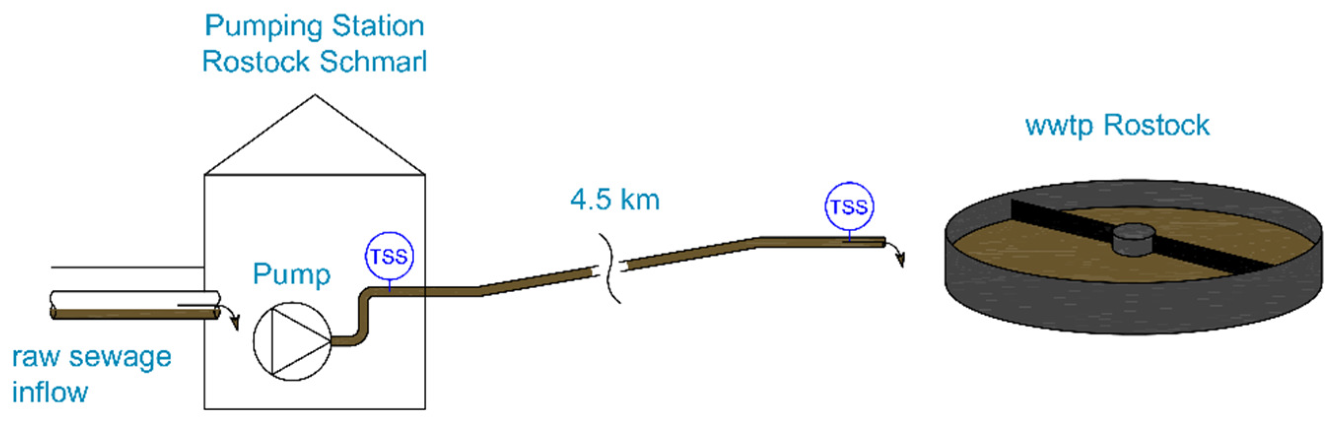
The supervision of solids transport under an energy efficient pump control was implemented in pumping station (PS) Rostock-Schmarl in the city of Rostock (northern Germany). PS Rostock-Schmarl conveys the raw sewage of ≈40,000 inhabitants directly, via two cast iron pipelines of 600 mm diameter and 4500 m length, to the central wastewater treatment plant (wwtp) in Rostock, by four pumps of 220 kW total pump power. The incoming sewage is filtered by a 20 mm rake at the inflow side of the PS. Under dry weather inflow the total suspended solids (TSS) concentration usually ranges from 150 mg/L up to 350 mg/L. The upstream, usually separating sewer sums up to 80 km. Under rainfall, the main roads storm runoff is connected to the upstream sewer (total suspended solids concentration then increases to >500 mg/L). A parallel storm sewer receives the residual surface and roof runoff. Additional information about the study area are provided by [
1,
2,
3] which includes a detailed schematic view of the sewer system and PS Rostock-Schmarl.
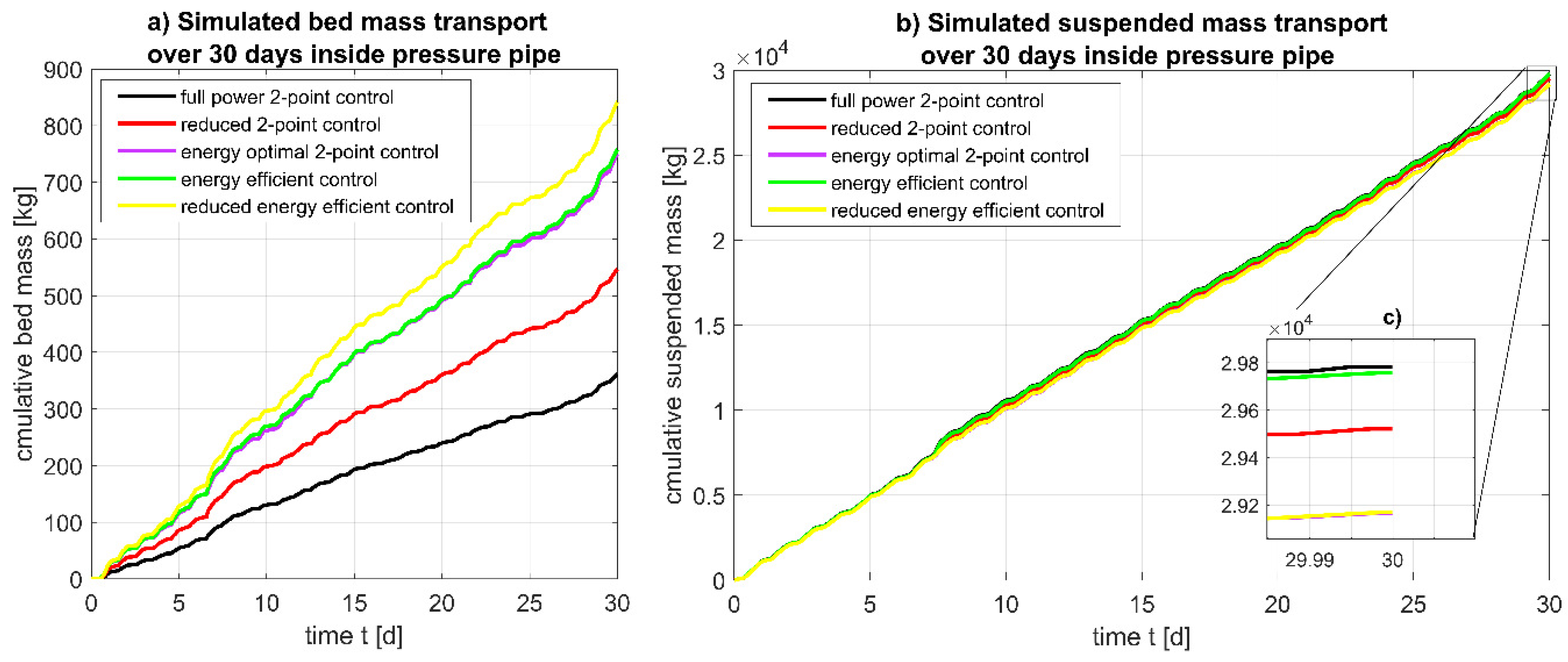
The usual operation mode of PS Rostock-Schmarl is a conventional two-point operation, where pumps switch on and off at pre-defined water levels inside the pump sump (sloped, squared geometry with a volume of 178 m
3). When pumps switch on, the variable frequency drive guarantees a soft start of the pumps. After a one minute soft start, the pumps operate at a defined duty point. In full power mode, the pumps duty point is then at ≈166 L/s (head loss ≈ 18.3 m) by ≈0.6 m/s flow velocity, respectively. The usual operation mode is the reduced two-point control where the flow decreases down to ≈100 L/s (head loss ≈ 17 m) by ≈0.35 m/s flow velocity, respectively. For a studied period of one year, an energy saving operation was implemented, to control two pumps and enhance energy efficiency. At low inflow, the duty point decreases to ≈76.5 L/s (head loss ≈ 16.7 m) at 0.27 m/s flow velocity. Energy savings amount to 11% compared to conventional operation. The following constraints mainly hindered additional energy savings: (i) minimum flow rate of ≈53 L/s (flow velocity ≈ 0.2 m/s) and (ii) pumps forced were to start up to maximum flow in each pump sequence, before regulating down to energy efficient flow. These rules are defined by the operator to ensure solids transport and to avoid blockages. For detailed information about the control modes, read [
1,
22,
23].
In parallel, measuring TSS by two turbidity sensors directly inside the pressure pipe (one at pumps pressure side and one at the outflow side in wwtp Rostock) ensured a continuous monitoring of solids transport. Furthermore, the measurements provided data for continuous determination of solids settling and erosion characteristics and subsequently data for model calibration. The monitoring system is explained in depth in [
3].
Figure 1 shows a simple schematic view of the study side.
2.2. Sediment Transport Basics
The transportation of solids inside a fluid is mainly influenced by two main physical effects: (i) sedimentation and (ii) erosion. Equally to those two effects, two operation modes can be distinguished in pressurized flow: (i) pump pauses (shut-off mode), where only sedimentation occurs, and (ii) pump sequences (shut-on mode), where solids eroded and subsequently transported under adequately hydraulic conditions.
In pump pauses, solids are settling according to their settling velocity at different speeds, mainly determined by their density and size. The sediment layer at pipes invert is then a superposition of different solid fractions. The settling behavior of various particle fractions can be described as a settling velocity distribution, as conducted in [
1]. The computation of several particle fractions is useful for dealing with pollutant transport when specific fractions contain more pollutants than other components (see [
24]). However, modelling various velocity classes also requires larger coding and computing effort. In contrast, pure mass growth of solids, when only TSS fluxes are of interest, can be modeled and calculated easily as an appropriate solution of a usual differential equation, e.g., as an exponential decay of solids concentration inside the fluid, as introduced in [
3].
In pump sequences, solids eroding due to the force exerted by the turbulent fluid flow inside the pressure pipe (Reynolds number of 240,000 at 0.4 m/s flow velocity). The force is expressed by the shear stress τ (N/m2) or indicated more exactly by the bed shear stress. When pumps speed up, flow velocity increases until τ reaches the critical shear stress level of the particles τcrit (N/m2). Because of the different densities of particles, solids are eroding successively after τcrit level of the lightest particle fraction is reached, until all particles are eroded. Solids are then transported either as bed load (sliding, rolling, and leaping of single particles) or suspended load, where particles are following the swirled streamlines of the turbulent flow. Suspended solids are then also moving transverse to the flow direction. The physical processes within the erosion are by far more complex as pure sedimentation of particles. So, the implementation into a simulation results in high computation effort. If the flow is always turbulent (here Reynolds number of 120,000 by a minimum flow velocity of 0.2 m/s) and only a mass balance is required for a simulation, swirls and micro effects can be neglected.
2.3. Mathematical Approximation
The solid transport is simulated for the above described pressure pipe (length
l = 4500 m, diameter
d = 0.6 m), conveying (mechanical pre-treated) raw sewage and sequentially combined sewage to the wwtp Rostock. The mathematical model is based on the advection-dispersion equation, Equation (1).
In Equation (1), the advective transport is represented by the first term
(kg/(m
3 s)), the dispersive transport is represented by the second term
(kg/(m
3 s)), and the reaction of a substance is represented by the third term
r (kg/(m
3 s)). With
u being the concentration of a substance to be transported (kg/m
3),
t the time coordinate (s),
v the flow velocity in flow direction (m/s),
x the space coordinate (m), and
Dxx the dispersion coefficient (m
2/s). The reaction of substances
r is defined by Equation (2). With
P being the production of a substance to be transported (kg/(m
3 s)) and
S the sinking or degradation of a substance to be transported (kg/(m
3 s)).
The complex physical processes during sedimentation and erosion are unnecessary for pure modelling of the sediment flux. Hence, the following simplifications are assumed for the simulation. The sedimentation of different solid fractions, as described in [
1], is not considered. The settling process is described as an exponential decay of solids, similar to [
3]. This minimizes the particle fractions to simulate and approximates the settling of solids adequately. The erosion of solids is described by a single particle fraction as well. Once eroded, the particles are distributed homogeneously over the pipes bottom, as the mean flow velocity is uniformly distributed over the pipes cross section in the model. As already mentioned in [
15] (p. 193) “longitudinal dispersion is usually not an important transport mechanism under most operating conditions” (with regard to dissolved substances). As a result, dispersion effects of contiguous grid sections is neglected completely (similar to [
15] p. 193). Further simplifications are: No attention is paid to biogenic processes inside the fluid or deposits phase, the pipes geometrical shape is ignored as the 1 D sediment transport is computed in longitudinal direction, the pipes negative or positive slope, and curvature has been ignored too. As a result of the simplification, the advection-dispersion equation simplifies to the one-dimensional advection equation with only the production and sinking left, Equation (3) (similar to [
15] p. 193).
The transportation of solids is simulated as a mass balance (conservation of mass) for the suspended load and bed load along the pressure pipe. Equation (4) describes the conservation of mass for suspended load transport. Equation (5) describes the conservation of mass for bed load:
The suspended load transport is defined as feeding minus loss. Therefore, the production P is replaced by the erosion of solids a(w,v) (kg/(m s)) and the degradation S is replaced by the particle loss inside the fluid s(u) (kg/(m3 s)). Thus, eroded mass per pipe length and time a(w,v) divided by pipes cross section A (m2) minus the particle loss inside the fluid s(u) represents the suspended load.
The bed load (Equation (5)) is as well defined as feeding minus loss. Here, the feeding is described by the particle loss
s(u) multiplied by
A minus the eroded mass
a(w,v). Erosion
a(w,v) is described by Equation (6), with
τpipe(v) (N/m
2) the current bed shear stress inside the pressure pipe,
τcrit(w) (N/m
2) the critical shear stress level of the raw sewage dependent on the particle mass on pipes invert
w (kg/m) and the erosion parameter
d (s), which describes the strength of the erosion (see [
2]).
The sedimentation is described as a first order decay process modeled by Equation (7).
The differential equation is approximated by the particle loss
s(u) by Equation (8), with the settling parameter
α (1/s), which determines the exponential decay and the particle concentration inside the fluid section,
u (kg/m
3) (see also [
3,
25]):
2.4. Numerical Method
The partial differential equations (PDE) are solved by a finite difference method (FDM) (partial derivatives are approximated as finite differences). FDM’s within water-quality modelling were i.a. investigated by [
26]. The authors conclude, that the FDM method is, next to others, “capable of adequately representing observed water-quality behavior” ([
26], p. 146).
The FDM method applied here is an explicit/implicit finite difference scheme centered in time (discretization in time) and backward in space (discretization in space). The centered in time scheme taking the average value between time steps n and n + 1 (also known as the Crank–Nicolson scheme). The first value n is calculated based on the previously computed value n − 1 (explicit), while the second value n + 1 is calculated based on the formerly computed value n within the same time step (implicit). The advective transport with the mean flow velocity results in the backward in space (or upwind) scheme, where only transport in the flow direction (from backward grid point) is allowed.
For the 1 D sediment transport model, the pipe is separated into 900 segments, with a length of ∆l = 5 m. For a stable solution, the Courant–Friedrichs–Lewy condition is defined as . The time increment ∆t for a simulation step is then defined as . Hence, the advective transport cannot be faster than one grid point per time step. Assuming a flow velocity of v = 0.5 m/s, the time increment of a simulation step is then calculated to ∆t = 10 s.
The numerical simulation is realized in several Matlab functions. The pump control strategies of PS Rostock-Schmarl (several regular and energy efficient control modes) are implemented into the transport simulation to investigate the particle transport under various control modes. Hence, the sediment transport simulation is based on the mean flow velocity, computed by a previous pumping simulation.
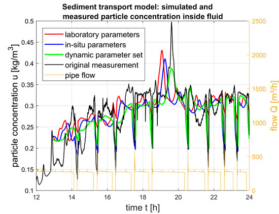
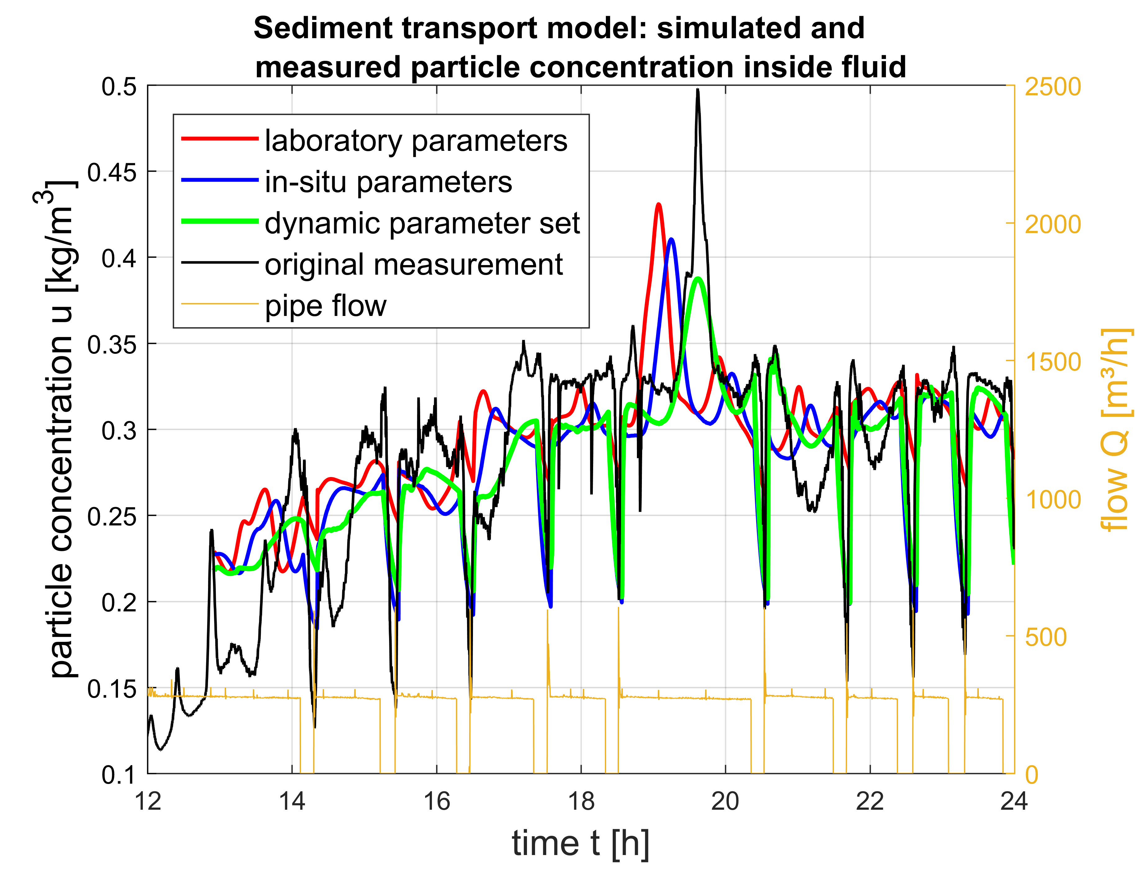
2.5. Calibration Parameters
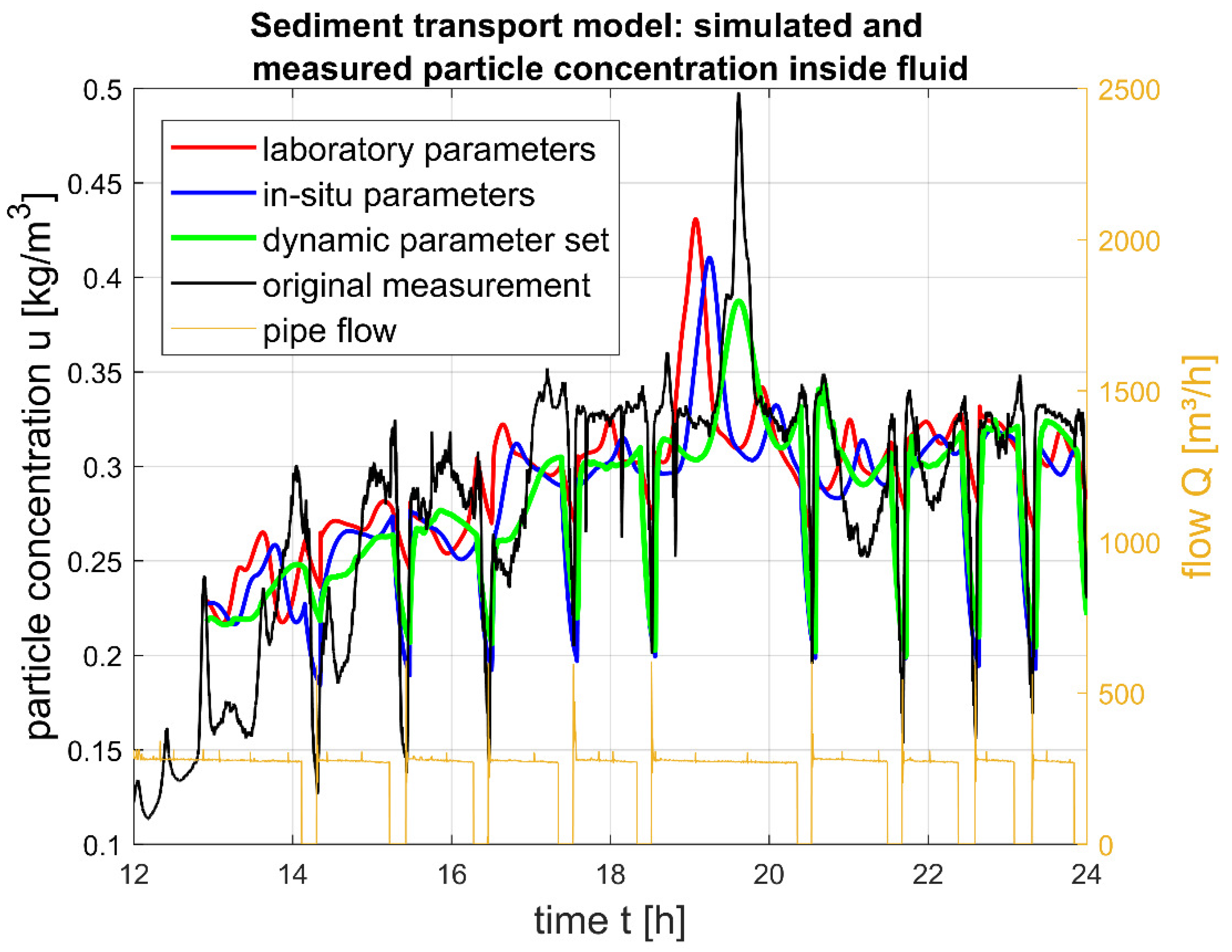
As described by Equations (6) and (8), the parameters α, d, and τcrit are mainly responsible for the sedimentation and erosion behavior and subsequently important for model calibration. The calibration of the transport simulation is based on two parameter sets: (i) ex situ parameters, resulting from laboratory experiments and (ii) in situ parameters, resulting from continuous turbidity measurement.
Ex situ parameters are provided by laboratory experiments, dealing with sedimentation [
1] and erosion [
2] of raw sewage samples from PS-Rostock Schmarl. Both experiments are explained in a few words: (i) the sedimentation tests are conducted in a vertical cylinder, the deposited mass is determined after various settling durations, and the main outcome are growth curves for settled solids mass. (ii) the erosion is tested in a vertical cylinder, the raw sewage is stirred until particles eroding from the ground level, the resulting erosion rates are detected by a continuous turbidity measurement, and the calibration parameters are derived from the growth curves and erosion rates. Hence, the parameters are based on a great simplification of real-world conditions. For the settling parameter
α, values between 0.0036 s
−1 and 0.032 s
−1 were determined, for settling periods of 24 h. The erosion parameter
d was determined between 0.057 s and 0.56 s after settling for 24 h.
Another calibration parameter is
τcrit. The critical bed shear stress defines the erosion limit and depends on the previous settling duration (long settling periods resulting in high
τcrit values). The determination of
τcrit results in values of 0.08 N/m
2 for settling periods up to one hour and <0.2 N/m
2 for settling periods of up to three days (see [
2]). The bed shear stress inside the studied pressure pipe is calculated by Equation (9), based on the fluid density
ρ (kg/m
3), the flow velocity
v (m/s), and the friction factor
λ (calculated by the Colebrook–White equation).
τpipe is calculated for the minimum flow velocity of ≈0.2 m/s to ≈0.1 N/m
2. Hence, the minimum flow velocity reaches the
τcrit value for one hour prior settling (0.08 N/m
2). At PS Rostock-Schmarl, pump pauses above one hour are prevented by a control regulation: At least one pump starts per hour to avoid blockages. But due to pumps soft start, the motor speed is regulated from zero flow up to full flow within 60 s, which results temporarily in flow velocities <0.2 m/s. To always have the correct
τcrit value before pumps start,
τcrit is implemented into the simulation as a function of the prior settling duration. The present value of
τcrit is received during the simulation by an interpolation between the laboratory
τcrit results of [
2].
The second parameter set are the in situ parameters, provided by a continuous turbidity measurement, as described in [
3]. Mass growths and erosion rates are determined inside the pressure pipe, as the pump pauses and pump sequences representing the settling and erosion experiments, respectively. By this, a wide range of calibration parameters are derived under real world conditions. After analyzing 6733 single settling events (or pump pauses), the settling parameter
α is calculated to an average value of 0.0026 s
−1. The erosion parameter
d is calculated to an average value of 0.018 s, after an analysis of 6653 single erosion events (or pump sequences).
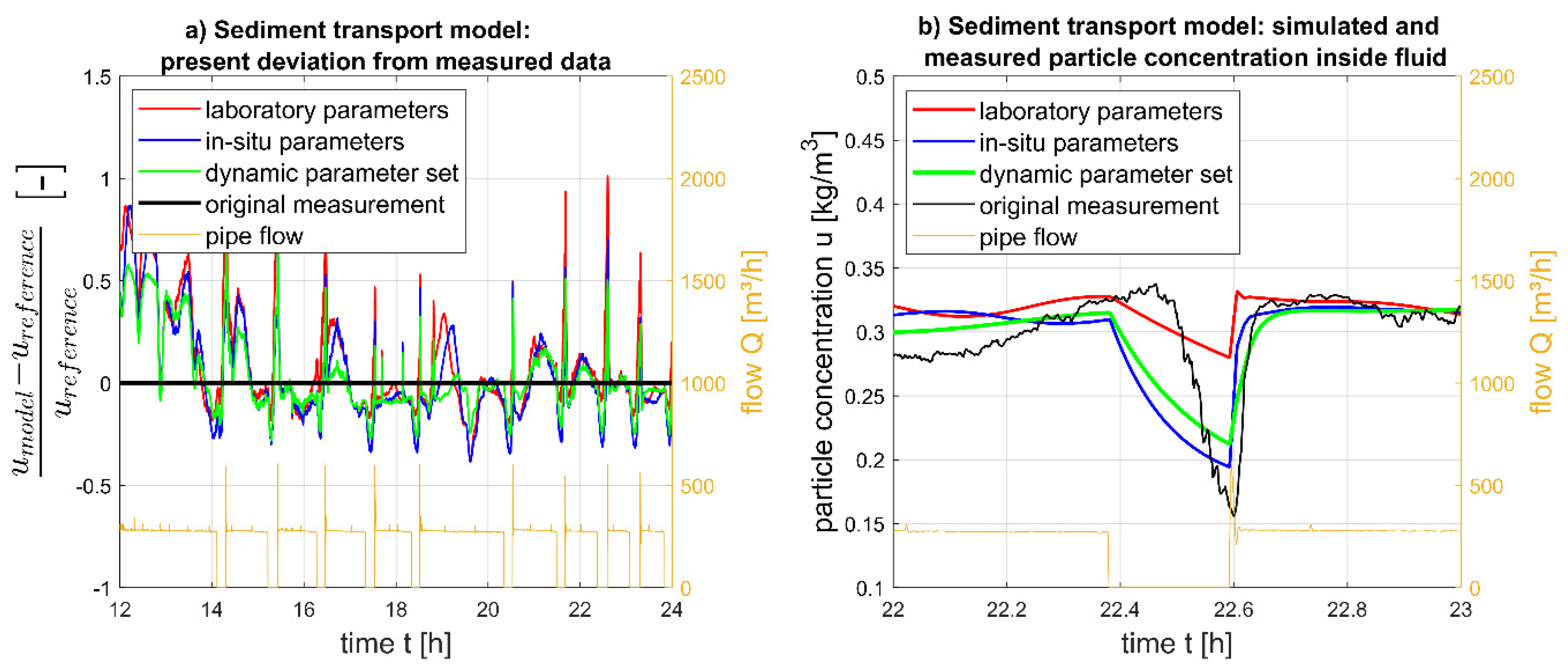
However, due to the large number of events, a much more precise classification than pure average values can be achieved. In [
3], a diurnal variation of the settling and erosion behavior along with the variation of the inflow rate (and accordingly the TSS inflow) was detected. The changing settling and erosion behavior are reflected by the settling parameter
α and the erosion parameter
d. Hence, if the transport parameters dynamically change with the TSS inflow during simulation, the model always computes the appropriate settling or erosion process. After combining the settling parameter
α of each single settling event (6733 in total) to the present TSS value, a simple linear function derives, Equation (10), with
uinflow (mg/L), the TSS inflow concentration.
The erosion parameter
d changes proportionally with the settling parameter
α. The ratio is determined to 1/0.1902.
d is then calculated by Equation (11).
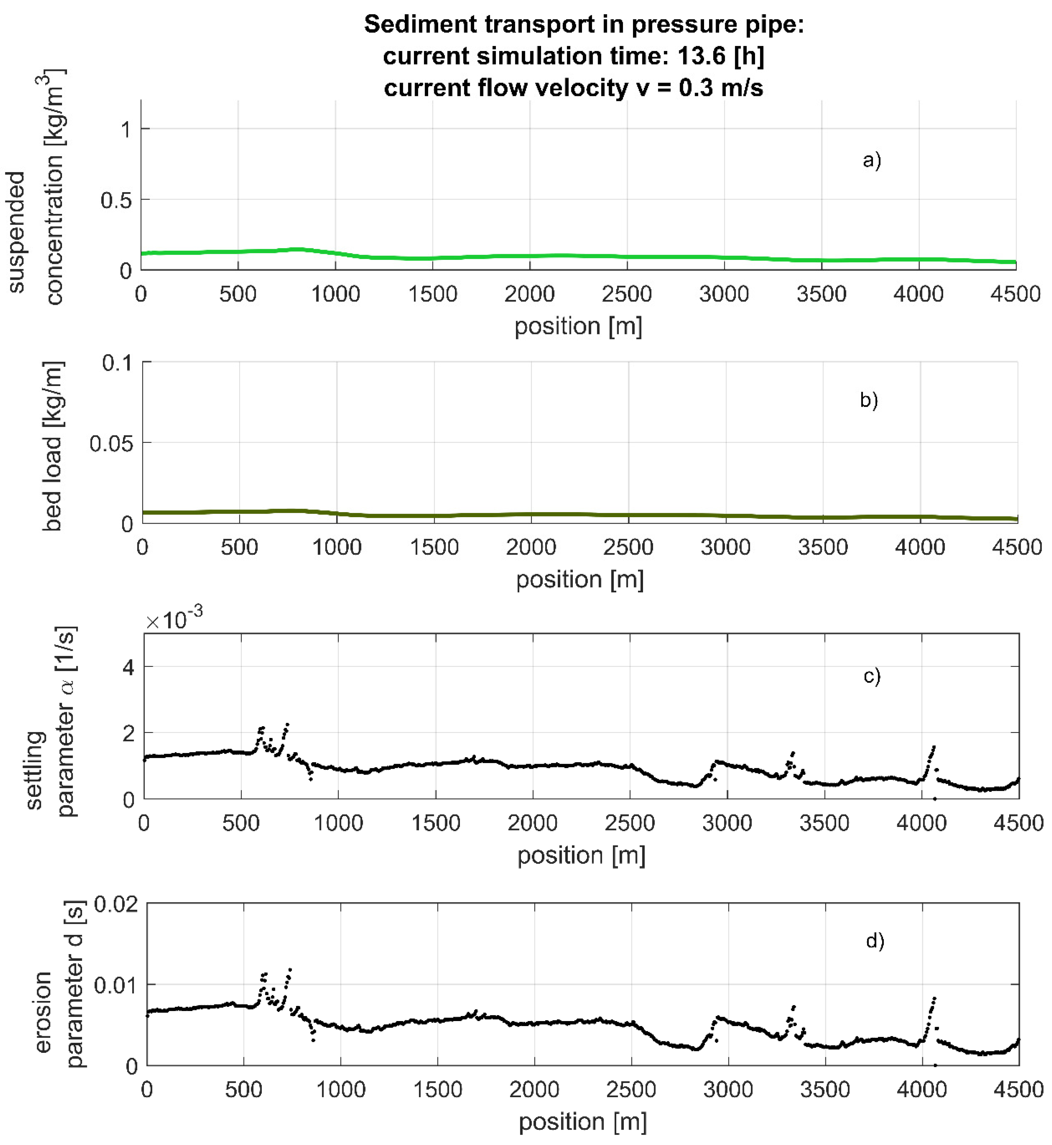
To illustrate the continuous adaptation of the model parameters,
Figure 2 shows, exemplarily, the status bar of the sediment transport simulation. At the current simulation time 01:36 p.m. the pumps generate a flow velocity of 0.3 m/s.
Figure 2a–d show the simulated values for suspended load (
Figure 2a), bed load (
Figure 2b), the settling parameter
α (
Figure 2c), and the erosion parameter
d (
Figure 2d) over pipe length (4500 m).


