Runoff Losses on Urban Surfaces during Frequent Rainfall Events: A Review of Observations and Modeling Attempts

Abstract

Quantifying urban runoff during frequent rainfall events is a key element in quality management of urban water due to their high contribution to the annual runoff flow. This explains the growing interest among hydrologists in studying runoff flow on urban surfaces. In this paper, we review most of the experimental approaches as well as the modeling ones conducted in the literature to understand and estimate runoff flow on urban areas. This review highlights the incoherence between our current understanding of the hydrological behavior of urban areas during frequent events and our conception of the loss functions in the urban drainage models. Field studies provided more insight into the determinant processes occurring on the different surface types during frequent events with depression storage being a fundamental element varying between surface types and for the same surface type and infiltration process being relatively important on paved areas especially in their cracks that constitute preferential pathways for rainwater. Analyzing a wide range of urban drainage models showed that these elements along with the temporal evolution of the hydrological behavior of urban surfaces due to seasonal and state conditions are not fully integrated in the models’ structures, which were initially developed for heavy rainfall events. Adapting the assumptions of urban drainage models based on these new factors must improve the performance of hydrological models for frequent rainfall events.

1. Introduction

In a context of growing awareness of the detrimental impacts of urban runoff contamination on receiving water bodies [1,2], more research and operational efforts are being invested in the management of urban stormwater quality. Urban drainage has since seen the development of a large variety of control techniques in response to the significant evolution of the stormwater management paradigm over the last few decades [3,4,5,6]. Among the latest techniques developed in this respect are the Low Impact Development devices (like infiltration trenches, vegetative swales, green roofs …), whose objective goes beyond stormwater management to incorporate a wide range of social, sanitary and economic considerations [7,8]. Proper conception and implementation of these techniques and other strategies relies on a precise assessment of their efficiency and suitability in given hydrological conditions [3].

Given the complexity of processes governing runoff flow and the arduousness and high cost of the experimental approach to quantify it [9], numerical modeling offers a powerful decision-making tool to simulate urban catchment behaviors and select the most adapted management practice [10]. Most urban runoff models developed in the literature are typically structured by a series of two classes of functions: production functions and transfer functions [11,12,13,14]. The former simulates surface storage, infiltration, and evaporation, whereas the latter simulates overland flow, subsurface flow, and sewer flow. While the transfer processes can be described physically, the production mechanism especially on impervious surfaces is still deemed highly complex and far from being fully understood [15,16]. It is therefore modeled in a conceptual fashion involving a high degree of empiricism contingent on the conditions for which they are constructed [17]. These production functions were initially developed for extreme rainfall events to support the need of flood risk assessment and are hence not adapted to frequent rainfall events [18,19,20,21] that are crucial for water pollution management as they constitute a major part of the annual mass of pollutants drained into surface waters [22,23,24]. So, models used to assess the stormwater runoff quality should be capable of simulating catchment behavior during small events. These events are usually characterized by a rainfall depth small enough that only the impervious fraction of the catchment area contributes to its downstream flow. In order to properly simulate these events, it is necessary to improve our understanding of the production functions on the impervious surfaces and upgrade the conceptual structure of hydrological models accordingly. Recent technologies and measurement techniques have been employed in this research line to better characterize the phenomena governing the runoff production on urban areas [25,26,27].

Based on a comprehensive review of the latest experimental characterization of impervious runoff from one side and the different structures of urban runoff models from the other side, this paper explores the gap(s) between observations and modeling that could explain the inadaptability of these models with small events. The paper is organized in two main sections. The first section presents all the experimental findings on runoff flow on impervious surfaces. The second one reviews the different structures of urban runoff modeling in order to identify the assumptions that could be at the origin of their ineptitude for frequent events.

2. Experimental Assessment of the Physical Processes Governing Runoff Production during Frequent Rain-Event

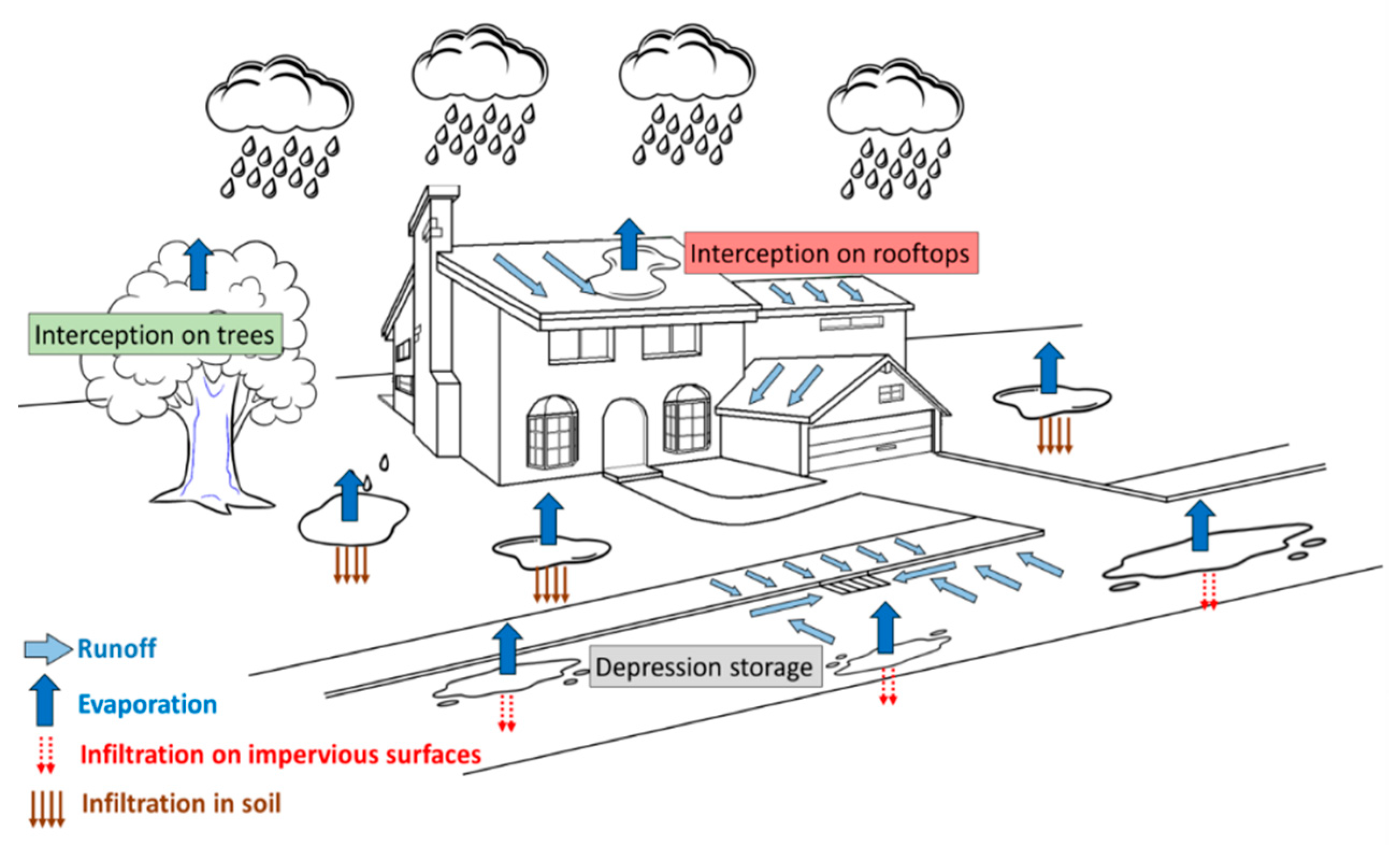
Runoff production represents the hydrological processes responsible for all the losses that rainwater undergoes when reaching the catchment surface before being conveyed by overland flow and sewer network to the catchment outfall. Urban catchments have a highly heterogeneous surface cover of structures and irregularities that form a buffer zone for rainwater falling on the catchment before evaporating or infiltrating. Rainfall exceeding the retention and infiltration capacities of the different surface structures constitutes what we call net rainfall, excess rainfall or effective rainfall that actually contributes to the outfall runoff. These production functions start with the beginning of the rainfall event and last for a shorter or longer period of time in function of the characteristics of the retention structures and the rate of input (precipitation) and output (evaporation and infiltration) flows. So, the runoff volume results from a complex interaction of different hydrological processes that are usually broken down into three processes: retention, evaporation, and infiltration. In this paragraph, we present a review of the experimental studies realized in the literature to evaluate the relative contribution of these processes to the runoff losses on urban impervious surfaces.

2.1. Retention

Rainwater retention occurs on the whole urban catchment with varying degrees of magnitude depending on the macro- and micro-morphological characteristics of the retaining surface. The retained volume is then drained by infiltration and/or evaporation. Based on the processes acting on this volume, a distinction could be made between two kinds of retention: rainfall interception where water is exposed only to evaporation, and depression storage where water is exposed to both evaporation and infiltration (Figure 1).

2.1.1. Rainfall Interception

Rainfall interception is defined as the part of rainfall retained by aboveground objects until it returns to the atmosphere through evaporation [28]. This process mainly occurs at the early stage of the rainfall event with a rate that rapidly approaches zero [29]. Urban areas are characterized by complex geometry of natural (vegetation) and artificial (buildings) canopies that participate in this process (Figure 1) and make interception observations difficult to realize. Thus, the difference between the input rainfall and output runoff measured on typical urban structures has always been used to deduce the intercepted rainfall volume sometimes represented as the evaporated quantity.

Rooftops

The analysis of rainfall and runoff volumes on one flat and two pitched roofs in Hertforshire [30] showed that runoff is only initiated by storms of at least 0.25 mm depth for both flat and pitched rooftops. Water fluxes were quantified in [31] (rainfall, runoff and evaporation) from six roofs with different slopes and orientations. The water balance between the input rainfall and output runoff was used to deduce the output evaporation, which was assumed to be representative of the amount of water soaked up by the roof surfaces, and eventually released back to the atmosphere by evaporation. The average of monthly contribution of evaporation process (in other words the initial abstractions) to runoff losses was found to vary between 9.5% and 41.9% with an average of 28% of the rainfall. Rainfall interception was investigated by [29] on a Comprehensive Outdoor Scale Model (COSMO) made of cubic concrete blocks uniformly spaced to represent an ideal building-street urban configuration. The study estimated rainfall interception on individual surface scale and on catchment scale. The local interception of each surface type (roofs, walls, and streets) was made by artificially pouring water onto these surfaces and then using a towel to estimate the maximum retained volume. The global interception was based on an event scale analysis attributing all the residues of input rainfall to the interception process whose contribution was found to vary between 0 and 5.1 mm constituting on average 6% of the gross rainfall depth. For weak events characterized by a rainfall depth less than 10 mm and average rainfall intensity less than 1.3 mm/h, high interception values were recorded reaching 48% on average. Events with rainfall depth less than 0.5 mm did not generate any runoff. Runoff from four different rooftops was studied in [32] to estimate their potential for rainwater harvesting. For 25 monitored storm events, the interceptions observed on sloped clay tiles (CT) and flat gravel (FG) were 0.8 and 3.8 mm respectively, whereas inclined metal (M) and plastic (P) roofs retained a negligible volume assumed to be zero. All the observations of rooftop interception found in the literature are recapitulated in

Table 1. Retention measured on urban structures (expressed as water depth by unit of surface during a frequent rain-event).

Retention	Reference	Estimation Method	Surface Type	Interception (mm)
Rainfall interception on rooftops	[30]	Intercept value with the rainfall axis in rainfall-runoff regression	Flat asphalt roof	0.37
			Front pitched roof	0.11
			Garage-side pitched roof	0.39
		Minimum event generating runoff	Flat asphalt roof	0.25
			Front pitched roof	0.25
			Garage-side pitched roof	0.25
	[29]	Difference of towel weight before and after using it to absorb water poured on the studied surface	Concrete rooftops	0.24
		Difference between rainfall depth and runoff depth	Outdoor scale model of 4 concrete blocks (buildings)	0–5.1
		Minimum event generating runoff		0.5
	[32]	Intercept value with the rainfall axis in rainfall-runoff regression	Sloping Clay tiles (CT)	0.8
			Sloping metal roofs (M)	0
			Sloping plastic roofs (P)	0
			Flat gravel roofs (FG)	3.8
Rainfall interception on urban trees	[33]	Difference between gross rainfall above canopy and net throughfall below canopy	Douglas-fir	20.4
			Western red cedar	32.3
	[34]	Difference between gross rainfall above canopy and net throughfall below canopy	Quercus ilex tree	0.26
	[35]	Difference between gross rainfall above canopy and net throughfall below canopy	Ficus benjamina tree	1.5
	[36]	Difference between gross rainfall above canopy and net throughfall below canopy	Oaks and pines	2.6
	[37]	Difference between gross rainfall above canopy and net throughfall below canopy measured with the aid of an artificial catchment	Pear tree	1
			Oak tree	2
	[38]	Rainfall simulator and electronic weighing balance	Platycladus orientalis	Cmin = 0.38 Cmax = 0.88
			Pinus tabulaeformis	Cmin = 0.43 Cmax = 0.85
			Quercus variabilis	Cmin = 0.17 Cmax = 0.30
			Acer truncatum	Cmin = 0.46 Cmax = 0.59
	[39]	Rainfall simulator and electronic weighing balance	Broadleaf deciduous	0.77
			Broadleaf evergreen	0.78
			Coniferous evergreen	1.25
Depression storage	[30]	Minimum event generating runoff	Traditional pavement	1
	[40]	Input volume before the onset of runoff	Six sections of residential roads with their curbsides	0.5–10.5
	[41]	-	Traditional pavement	0.2
	[26]	Terrestrial Laser Scanner (TLS)	Traditional pervious pavements (Limestone, sandstone, red brick blocks)	0.08–0.58
			Modern pervious pavements (Granite blocks, concrete, natural stone, rubber blocks…)	0.07–0.22
			Modern infiltration active (concrete paving)	0.56–1.41
			Non-pervious asphalt	0.08

.

Urban Trees

Considerable research studies were conducted on the impact of tree interception on hydrological processes in naturally forested areas. They reported a wide range of interception loss depending on forest structure, canopy structure, and meteorological factors: between 20–40% in coniferous and between 10–20% in deciduous forests on annual scale [42,43]. The effect of urban trees on rainfall interception is however rarely quantified and the observations made in forested areas cannot be applied on urban areas due to the different conditions between the two contexts (available growing space, edge effect, isolation, wind penetration, canopy cover, age, diversity, and microclimate …) [35,44,45].

In almost all studies conducted in urban conditions, interception loss was estimated as the difference between the gross rainfall (the amount that would reach the ground in the absence of the tree) and the volume that actually fell under the tree crown with some differences in the way each volume was measured. Interception by two tree species was measured in [33]: Douglas-fir and Western red cedar in variable landscape sites (streets, parks, and natural forested areas). The average canopy interception during seven rainfall events for Douglas-fir and Western red cedar was 49.1% and 60.9% corresponding to an average net loss of 20.4 and 32.3 mm respectively. The extremely high values obtained in this study are majorly attributed to the very long durations of the sample rainfall event (between 15 h and 179 h). Interception loss by an isolated Quercus ilex tree was estimated by the difference between gross and net rainfall monitored below the tree crown over 2 years [34]. Total interception reached 22% of the gross rainfall with a canopy storage capacity estimated at 0.26 mm per unit of crown-projected area. Very high interception losses were found in [35] on an isolated Ficus benjamina tree in urban area. The total interception on 19 rainfall events was found to be 59.9% of gross rainfall with higher values (78–100%) recorded for small events (<8.4 mm). Canopy saturation was estimated at 1.5 mm, and the average time of saturation was around 19.5 min using the inverse procedure of Rutter’s model describing rainfall interception by vegetation. In [46], the impact of trees on surface flow on urban areas was assessed by comparing the runoff measured on an asphalt plot and that measured on an asphalt plot with a tree planted in the center. Trees and their associated tree pits were found to reduce runoff by as much as 62%. However, these results cannot be attributed purely to interception but to the mixed effect of interception and infiltration in tree spit. Rainfall interception by deciduous oaks and pine trees in 16 residential yards was quantified in [36] for 14 rainfall events. During 14 rainfall events, 9.1% of the total gross rainfall was intercepted by these trees representing on average 19.9% per event. Two trees planted in an urban street setting made the object of an experimental study during a 5-month period [47]. E. nicholii, having dense canopy, intercepted more of the smaller rainfall events so that 44% of the annual rainfall was intercepted as compared to 29% for the less dense E. saligna canopy. The variation of canopy interception as a function of rainfall characteristics was also studied. E. nicholii was able to intercept the majority of rainfall events that are <4 mm, whereas the thinner more sparse canopy of E. saligna intercepts less than 40% of even small rainfall events <2 mm.

An upgraded measurement system was tested in [37] by constructing an artificial catchment beneath a 9-year-old pear tree and a 8-year-old oak tree with a collection area extending beyond crown edges to monitor rainfall interception during 3 years. Interception losses accounted for 15% of gross precipitation for the pear tree and 27% for the oak tree. Analysis of temporal pattern of interception indicated that it varies from 100% at the beginning of the rainfall event to about 3% at maximum rain intensity.

In [38], researchers used a rainfall simulator and an electronic weighing balance positioned above and below four trees of four different species to measure the interception during a wide range of rainfall conditions and examine the effect of rainfall traits and crown structure on interception process. Results indicated that interception is a dynamic process that evolves in three phases: (1) wetting phase during which the dry crown intercepts rainfall till, reaching its maximum capacity (Cmax); (2) saturation phase where no more rainfall is intercepted; and (3) drainage phase following the rainfall event during which a percentage of the retained water drains off to reach the minimum interception storage (Cmin). Cmax and Cmin were found to be highly dependent on the tree species and rainfall intensity. In [39], the same measurement system was employed (rainfall simulator and digital balance) to measure surface storage capacity of 20 urban tree species. Eight samples were taken from each species and 12 rainfall intensities were simulated. The mean value of rainfall interception among all species was 0.86 mm.

2.1.2. Depression Storage

Rainfall volume trapped in depressions present on urban surfaces held until it infiltrates or evaporates is referred to as depression storage (Figure 1). The process of filling depressions is relatively fast and is a function of the depression capacity, precipitation intensity, evaporation, and infiltration rates, and is in the order of seconds to minutes [48]. Direct measurement of depression storage is hardly accessible and thus indirect methods are usually used to estimate this quantity. Road runoff was studied in [30] on a section in Hertforshire, England. A storage capacity of 1 mm was estimated from the minimum rainfall event causing runoff. Nehls et al. [26] is one of the few studies using a direct method to quantify the surface storage on pavements. They employed a terrestrial laser scanner (TLS) on 11 ideal typical urban paved surfaces of different materials having a 2% slope and that had never been subjected to human or car loads. Measured values range between 0.07 for granite paving blocks to 1.4 mm for concrete pavement with infiltration joints. A systematic underestimation of 30% was noted in the laser scanner measurements relative to direct measurements. In [40], a few irrigation experiments were carried out on six sections of residential road to study the runoff on paved areas and determine runoff losses including initial losses. Depression storage was deduced from the volume sprayed before runoff started. Mixed results were obtained with two sections (4 & 5) behaving in a classical manner, two others (2 & 3) with highly variable initial losses, and the last two (1 & 6) showing no reaction to irrigation flow exceeding their initial loss estimated from other experiments. The significant variability of depression storage reaching up to two orders of magnitude (0.07–10.5 mm) reflects the complexity of this phenomenon, whose variability depends on multiple factors related to site and events characteristics. Despite the latest technological advances of measurement techniques, quantifying depression storage is still one of the most challenging tasks for hydrologists. The difficulty in distinguishing this process from other surface processes especially infiltration explains why experimental measurements of depression storage are rarely available in the literature (Table 1).

All the experimental results of the literature reviewed in this part reveal the important contribution that the retention process could have to runoff losses during small rainfall events as retention values were found to be of the same order of magnitude of rainfall height of a small event. These results also prove that retention is still neither easily commensurable nor fully understood due to its high multifactorial variability. Retention values measured on different urban surfaces (Table 1) are found to be extremely variable from one surface type to another and even for the same surface type when different measuring methods are applied or different rainfall events samples are studied. So, not only the surface type but also its geometrical characteristics and the rainfall events sample influence the retention capacity. However, among all these parameters, some were found to be determinant for certain retention types. Surface slope was found to explain a big part of the rooftop interception [32]. Trees’ capacity of retention was proved to be highly dependent on their crown structure [38].

2.2. Infiltration

Urbanization has always been associated with rainproofing due to the very low permeability of urban soil covers from one side and their relatively smooth surface that shortens the residency time of the runoff flow from the other side. However, on asphalt and concrete pavements, the decrease of direct recharge from their low-permeability matrix might be offset by an increase in localized recharge through fractures and joints that provide potential preferential avenues for infiltration. For that reason, the effect of urbanization, especially the paved areas on the infiltration mechanism, is still not fully understood and has consequently made the subject of intensive research in recent years, which addressed it using direct or indirect measurement techniques [27].

2.2.1. Indirect Quantification

Among the indirect approaches, Davies [30] calculated the runoff losses during a rainfall event due to infiltration on paved surfaces as the residue of the water balance between the depression storage estimated from rainfall-runoff regression and the evaporation deduced from another mass balance analysis of an urban surface (asphalt roof), on which infiltration is considered zero. Of the total 83% runoff losses observed, infiltration was found to contribute to 36%. A similar approach was conducted by [47], which consisted in artificially irrigating some pavement sections of bituminous macadam with its curbsides and measuring the runoff rate at the outfall to deduce the continuous losses due to infiltration by subtracting the runoff rate from the irrigation rate when these two reached their steady state. Infiltration fluxes were found to be very important, and the infiltration rate was of the order of 0.36 mm/h. The water balance concept was also applied [49] to small-scale samples (300 mm × 300 mm) of various paving materials (concrete, brick paving, asphalt, and macadam) to assess the importance of runoff, evaporation and infiltration processes on these surfaces. Results showed that infiltration in the road structure itself is very low (between 0 and 2% of the rainfall depth), but in the joints present between brick paving it was responsible for the most significant output (52%). Identical behavior was recorded for asphalt and concrete samples with almost 2/3 of the rainfall appearing as runoff, while the dense bituminous macadam detained 2/3 of the rainfall that were lost by evaporation, probably because of the surface texture. However, the experimental setup did not allow the evaluation of the impact of depressions and cracks in the paving materials on runoff losses.

2.2.2. Direct Quantification

Field experiments carried out by [50] on two small scale concrete and asphalt pavements having different slopes and for different rainfall intensities and durations recorded very high runoff levels of the total rainfall depth with infiltration losses not exceeding 2%. Using a double-ring infiltrometer, the permeability of asphalt, concrete, and asphalt-concrete pavements was estimated in [51]. High values of hydraulic conductivity were measured (

Table 2. Infiltration rate measured on different types of paved surfaces (mean value or min-max values).

Reference	Pavement Type	Infiltration Rate f (mm/h)	Method
[58]	Concrete road	7–27	Pavement irrigation
[47]	Bituminous macadam dressed by granite chippings	0.6–3.6	Mass balance between irrigation inflow and gully pot outflow
[59]	Paved area good state	0.036	Unknown
	Paved area slightly degraded	0.36	Unknown
	Paved area highly degraded	36	Unknown
[60]	Asphalt road	0.36	Variation of water content in all the layers of the pavement structure
[55]	Asphalt concrete plates	0.007–0.01	Lysimeter
[51]	Urban pavement:	2.1	Double-ring infiltrometer
	Asphalt pavement	2.9–76
	Concrete pavement	1.4–2404
	Combined	1.4–243
[56]	Urban pavement	1.08–21.6	Double-ring infiltrometer

), ranging between 1.43 and 2 405 mm/h, which is comparable to that of fine-grained sands, sandstones, silts, and loams. However, all sampled points have expansion joints or fractures, except three on which no infiltration was observed. Ragab et al. [52] measured infiltration on roads in residential areas using soil moisture sensors installed underneath paved structures and found 6–9% of the total annual rainfall infiltrate through these structures. Other studies [53,54] observed a direct relation between water content in pavement structure measured on long periods (3 years) and rainfall depth. Findings showed that the annual infiltration on the pavement surface represents 25–30% of the total rainfall depth with an infiltration rate of 0.36 mm/h equivalent to that of a silty soil. An urban lysimeter was developed in [25] to study the water budget on asphalt concrete plates of 0.5 m² extracted from in-situ roads that had been operating for 20 years. The method consists in measuring runoff, infiltration and storage variation to deduce rainfall and evaporation rates. Infiltration was almost negligible (between 2–3%) with 73% and 74% of rainfall converted into runoff flow. Complementary measurements of the hydraulic conductivity (Ks) were realized in an attempt to explain the weak role of infiltration in the hydrologic behavior of these plates [55]. Using the irrigation technique until reaching a steady infiltration flux, Ks was estimated at 0.007–0.01 mm/h, which is low compared to other values reported in the literature for the same type of surface material (Table 2).

2.2.3. Temporal and Spatial Variability

The infiltration process on paved surfaces is highly variable both in space and time. Infiltration losses measured on six pavements [47] showed a decreasing temporal evolution declining rapidly at the beginning to reach a stable rate until the end of the rainfall event (Figure 2). The double ring infiltrometer was used by [56] to carry out a series of infiltration measurements on five different points in a parking lot. High spatial variability was observed with the average permeability ranging between 1.08 and 21.6 mm/h (Table 2). Monitoring infiltration during rainfall event showed a rapid decrease of infiltration rate by one order of magnitude within 16 min as illustrated in Figure 3. An extensive investigation of the infiltration capacity of pavement structures was realized by [57] through lab tests and field measurements. Several types of pavements have been evaluated. Remarkably high infiltration rates were obtained even on pavements that are generally considered to be hardly permeable. Figure 4 illustrates numerous types of variability of the infiltration rate. It was found to exceedingly vary from one site to another irrespective of the particular type of the pavement and within each site. Another significant variability was also reported between the initial and final rate on each monitored point. Not only the values but also the temporal evolution of these rates (initial and final) vary among sites.

2.2.4. Influential Factors

Multiple factors have been identified in the literature for being determinant of the infiltration process on urban surfaces.

• Depression Storage: The presence of depression storages on paved areas is an influential factor on infiltration as water is held for a longer time and will thus be more subjected to infiltration [26].
• Mixture properties: The effect of the asphalt mixture properties on the pavement permeability was studied by [61]. Based on the experimental data collected on five sites, an exponential relationship was observed between field permeability and the in-place air voids. In this respect, the aggregate size was found to be significantly determinant for the air void ratio and hence the pavement permeability. Excessive permeability of 36 mm/h, 43.2 mm/h, and 54 mm/h were recorded for coarse-graded mixes having NMAS (Nominal Maximum Aggregate Size) of 9.5, 19, and 25 mm at an air void ratio of 7.7, 5.5, and 4.4 respectively. Based on controlled experiments in the laboratory, [62] highlighted the positive correlation between roads porosity and permeability. In [63], five types of asphalt mixtures were tested for their hydraulic conductivity using a dual mode permeameter. For open graded large stone mixture, the pseudo-coefficient of permeability varies between 9720 mm/h and 53,280 mm/h. For open graded drainable base, it varies from 88,920 to 129,960 mm/h. For dense mixtures, it varies from 10.8 mm/h to 417.6 mm/h. This coefficient showed an exponential variation in terms of the effective porosity.
• Pavement age: Some researchers were interested in studying the impact of a pavement age on its infiltration capacity. Contrasting results were obtained according to the pavement type. Based on in-situ measurements of infiltration on a classical cement pavement in Brussels over a 1 month period (November), Van Ganse (1978), cited in [60], noticed a clear increase in the pavement permeability with ageing. A slight degradation of the pavement state could increase the infiltrated volume of rainfall from 5% (rate observed for a new pavement) to almost 50%. Another observation made in [59] noticed a decrease by one to three orders of magnitude of the pavement permeability with increasing degradation. However, an inverse effect of ageing on pavement infiltration capacity was obtained when in-situ measurements were carried out on porous paving blocks and permeable interlocking concrete pavement [64]. Results of the field tests show a clear decrease in the long-term infiltration performance with age interpreted by the entrainment of mineral and organic fines responsible for the clogging of joints and pores of porous paving blocks. This recession was found to reach its asymptotic capacity after 8–12 years of the construction of these types of pavements.
• Cracks and joints: Numerous studies attributed the high permeability of paved areas to cracks and joints. The infiltration rates (7–27 mm/h) obtained by the irrigation experiment realized by [58] were much higher than those obtained in the laboratory experiments on solid road samples (0.5 mm/h). This result corroborates previous findings in [65] who explained the high infiltration rates by the fractures capacity of absorbing water. Extensive quantification of the fractures and joints permeability was carried out on 200 points on asphalt and concrete pavements using a double-ring infiltrometer [51]. High values of infiltration rates were recorded without showing any correlation with the aperture of fractures and expansion joints on either pavement. These findings were interpreted by the fact that fractures and joints are filled with sediments and thus the sub-grade permeability is the controlling factor of the overall pavement permeability.

2.3. Evaporation

Evaporation represents a major component of the global water balance [66]. It might be considerably less in urban areas than in rural ones, mainly due to reduced surface depressions leading to a lower quantity of water being retained and exposed to evaporation. This process does not participate directly in runoff losses, but intervenes in draining the depressions and interceptions to recover the surface retention capacity. Almost 21% of the annual precipitation falling on paved surfaces was supposed to be lost by evaporation process [30]. One of the reasons behind that is the increase in temperature of urban centers. Evaporation on paved areas was shown to occur in different compartments of the paved structure [67]: the upper surface storage of pavers, the porous matrix of pavers, the joints between pavers, the retained water in the surface depression, and cracks. In practice, evaporation is most often restricted to the uppermost compartment consisting of the pavement material and joints with the infiltrated water supposed to be shielded by the pavement structure [67]. A high-quality experimental setup was installed on an open parking lot [68] to meticulously measure all components of the water budget during artificial rainfall events generated by a sprinkler system. Of the 10 studied events, evaporation contribution was estimated at 17%. In their investigation of the hydraulic behavior of road structures on three car parks and one internal road, Ragab et al. [52] reported a seasonal variability of the runoff flow having annual average of 70% with a peak of 90% in winter and a minimum of 50% in summer. Given that infiltration was estimated to participate by 6–9% of annual rainfall loss, evaporation was therefore supposed to represent 21–24% of annual rainfall, with more evaporation taking place during summer than winter.

2.4. Bulk Runoff Losses on Urban Surface

Some studies were interested in evaluating the bulk runoff losses, which is an integral measure of all losses occurring on the entire watershed rather than individual surface scale. This type of approach usually distinguishes initial losses from continuous losses, the former is mostly attributed to retention processes, whereas the latter is mostly attributed to infiltration and evaporation. Around 763 storms on 26 urban basins located in 12 countries were analyzed in [69] using regression plots. Initial losses were estimated between 0 and 6.12 mm with an average value of 0.85 mm. Fifteen residential urban catchments were monitored for rainfall and runoff over a 4-year period [70] and then analyzed to estimate some impervious area parameters including the depression storage. A narrow range of [0–1.29] was obtained. Data collected on 18 urban European catchments [71] showed that initial losses deduced from rainfall axis intercept in a rainfall-runoff regression analysis ranges between 0.13 and 1.5 mm. Default values adopted by computer software (MOUSE, ILSAX, SWMM etc…) of urban drainage modeling are within the range of 0.5–2.5 mm with an average of 0.58 mm.

Many attempts are made in the literature to relate the bulk retention capacity considered to be representative of initial abstractions with the catchment characteristics in order to derive general relationships that could be used on ungauged sites (

Table 3. Regression relationship between retention capacity and catchment slope.

Reference	Retention Capacity = f (Slope)
[71]	$d_s=0.77 S^{-0.49}$
[72]	$d_s=k S^{-0.5}$ For pervious surfaces, $k=0.28$ For impervious surfaces, $k=0.71$
[73]	$d_s=1.075 S^{-0.27}$
[28]	$d_s=3.3-76.5 S$
Willeke (1966) cited in [74]	$d_s=4.1-100 S$
[75]	$\begin{array}{cc}{d}_s=a+b\left(3-S\right)& S\le 3\%\\ d_s=a& S>3\%\end{array}$ For pervious surfaces, $a=2, b=4$ For impervious surfaces, $a=0.5, b=1$

$d_s$ = retention depth [mm], $S$ = catchment slope [%].

). The parameter that comes out the most as an explanatory factor of the retention capacity is the surface slope. A good correlation was found between these two variables using power function on the 18 urban catchments studied by [71] (Figure 5). A similar regression relation was empirically determined and incorporated in the Wallingford Procedure [72] and is now commonly used in UK and Belgium to estimate maximum surface retention. The same power function gave also the best fit of retention capacity data against surface slope [73] but with different coefficients than those of [71]. Data collected on four small impervious areas near Baltimore [28] having a slope range between 1–3% showed that depression storage varies linearly as a function of the catchment slope (Figure 5). On another slope interval (0.7–3.4%), a similar linear relationship was proposed by Willeke (1966), cited in [74]. Chocat et al. [75] mentioned that a linear relation between retention volume and surface slope is applicable on pervious surfaces as well as impervious ones but with different coefficient values between the two surface types. Jovanovic [76] combined several experimental studies carried out on impervious areas and noticed a clear decrease in the storage capacity with increasing ground slope. However, these common results of the good representation of the retention capacity by the surface slope were contrasted by the findings of [70] where no correlation could be obtained between these two parameters.

Other studies were interested in evaluating the contributions of infiltration and evaporation to the continuous runoff losses. Howver, since these processes occur on a longer period of time than rainfall duration with even higher post-event contribution than during the event, these evaluations considered a large temporal scale (annual or seasonal) on which the retention process or the initial losses dissolve. Retention constitutes a temporary buffer rather than actual losses, but is sometimes considered as runoff loss when working on event scale as evaporation and infiltration of the retained quantity occurs after rainfall event. Findings of these studies represented in

Table 4. Observed annual hydrological balances of different paved surfaces with seasonal (summer and winter) values (F: Infiltration, R: Runoff, E: Evapotranspiration).

Reference	Pavement Type	Annual			Summer			Winter
		F (%)	R (%)	E (%)	F (%)	R (%)	E (%)	F (%)	R (%)	E (%)
[30]	Paved surface							36	17	21
Wessolek (1993, 1994) cited by [77]	Mosaic cobblestone	33	54	13	23	60	17	48	46	6
	Concrete paving slab	20	70	10	12	74	14	32	64	4
Wessolek (2001) cited by [67]	Asphalt road	8	72	20	8	69	23	9	75	16
	Concrete and cobblestones sidewalk	38	31	31	34	24	42	43	40	17
Diestel and Schmidt (2001) cited by [67]	Small granite stones	74	7	19
	Small cobblestones	67	9	24
	Interlocking concrete	78	10	12
	Rubber pavers	86	11	3
	Grass pavers	68	6	26
	Brick pavers	76	10	14
[52]	Asphalt car park	8	70	22
	Asphalt car park	9	70	21
	Block paving car park	6	70	24
	Asphalt road	6	70	24
[25]	Asphalt concrete	3	74	23
		2	73	25
[49]	Flat concrete slab							1	69	30
	Hot-rolled asphalt							0	56	44
	Inclined concrete slab							2	93	5
	Dense Bitumen Macadam							0	36	64
	Brickwork							54	9	37
Flotter (2006) cited by [77]	Concrete cobblestone	80	12	8	68	18	14	89	8	3
	Concrete paving slab	54	41	5	47	44	9	59	39	2
[77]	Small cobblestones	70	15	15	60	22	18	81	7	12
	Large concrete pavers	64	26	10	54	35	11	75	16	9

suppose that infiltration is dependent on pavement type, whereas evaporation is dependent on weather conditions. Classical asphalt pavement seems to absorb less rainwater (2 to 9%) than porous pavements, infiltrating up to 86% on rubber pavers and 89% on concrete cobblestones. Seasonal variability of infiltration contribution to runoff losses was found to be very weak on asphalt pavements and significant on porous pavements, always with higher contribution in winter than in summer. Inversely, evaporation recorded higher contributions in summer than winter with minor variability between different pavement types.

In conclusion, runoff losses are governed by two major processes: retention and drainage processes. Retention includes interception, which is the part retained by rooftops and plants and is drained only by evaporation and depression, which is the part retained by ground depressions and is drained by both evaporation and infiltration. Retention occurs mainly at the beginning of rainfall events and is thus considered as initial losses, whereas infiltration and evaporation contribute to runoff losses during and after the rainfall event and are thus considered to be continuous losses. Experimental characterization of retention processes showed relatively important retention values that are comparable to the rainfall height of small events. Contrary to former beliefs, site investigations revealed non-negligible rates of infiltration on classical pavement surfaces associated with high variability in space and time and attributed majorly to joints and cracks. Evaporation proved to contribute more than infiltration to runoff losses on classical pavements with higher rates in summer than winter.

3. Models and Uses of Runoff Losses on Paved Surfaces

The large variability of modeling approaches reported in the literature stems from the level of the physical representation of processes responsible of continuous losses. Two classes were identified for these runoff models according to the way they describe these processes: global approach and detailed approach.

3.1. Global Approach

Due to the complexity of the hydrological processes on urban catchments during rainfall events, many researchers adopted a global approach in quantifying the runoff losses by lumping them all into a single coefficient determined from the regression analysis of observed data of runoff flow and rainfall depth.

3.1.1. Model Structure

Without accounting for the initial losses, the approach is known as the rational method, which is the oldest method that is still used today to model rainfall-runoff transformation for its simplicity and widespread acceptance. In its original version, the rational method relates the peak runoff flow to the rainfall intensity, usually taken from Intensity–Duration–Frequency curve for a particular length of time (time of concentration), using a point runoff coefficient. However, this method was later applied on volumetric variables to determine the runoff volume rather than the peak flow out of the precipitation volume using a volumetric runoff coefficient. Since this coefficient depends on the land use, soil type, surface slope, rainfall intensity, and antecedent hydrological conditions, it varies in time and space and is thus taken as a constant average for the whole basin.

$$\mathrm{R}={\mathrm{C}}_{\mathrm{r}}\times \mathrm{I}\times \mathrm{A}$$

(1)

• $\mathrm{R}$ = Runoff volume [l³]
• ${\mathrm{C}}_{\mathrm{r}}$ = Volumetric runoff coefficient [-]
• $\mathrm{I}$ = Rainfall depth [l]
• $\mathrm{A}$ = Catchment area [l²]

However, this method is usually applied while accounting for the initial losses that are assumed either constant or variable from one event to another. In the second case, a complementary equation is needed to estimate the initial loss for each rainfall event as a function of its antecedent conditions. Some researchers [13] found that the potential evapotranspiration during the dry period preceding the rainfall event is capable of explaining the initial loss, and thus, established relationship between them. Alhoujayri [78] chose the antecedent dry weather period to explain the initial loss.

$$\mathrm{R}={\mathrm{C}}_{\mathrm{r}}\times \left(\mathrm{I}-\mathrm{IL}\left(\mathrm{ev}\right)\right)\times \mathrm{A}$$

(2)

• $\mathrm{IL}\left(\mathrm{ev}\right)$ = Initial loss of a certain storm event [l].

Other researchers considered that continuous runoff losses, especially infiltration, will decrease during a storm event and encoded this concept in their models using a variable runoff coefficient. Both [79,80] considered an exponential increase of the runoff coefficient (Figure 6) until no more runoff loss occurs when depressions are full, infiltration slows practically to nothing and evaporation becomes insignificant. In the hydrological module used in CANOE [81], runoff coefficient is considered to evolve as a function of the storm event characteristics taking three constant values according to the rainfall intensity (low, middle, high) (Figure 6).

$${\mathrm{C}}_{\mathrm{r}}\left(\mathrm{t}\right)={\mathrm{C}}_{\lim } \times \left(1-{\mathrm{e}}^{\mathrm{V}/\mathrm{K}}\right)$$

(3)

• ${\mathrm{C}}_{\mathrm{r}}\left(\mathrm{t}\right)$ = Instantaneous runoff coefficient (-)
• ${\mathrm{C}}_{\lim }$ = Maximum runoff coefficient attained when all depressions are saturated (-)
• $\mathrm{V}$ = Cumulative rainfall depth from the beginning of the rainfall event (l)
• $\mathrm{k}$ = Constant specific to the rainfall event (l)

Some attempts were made in the literature to establish relationships between event runoff coefficients and other parameters describing input rainfall and hydrograph characteristics. Mosini et al. [82] carried out a multiple regression analysis not on the event runoff coefficient but on the statistical one, which relates statistical values (quantiles) of the flow rate and rainfall intensity determined from QDF (Flow–Duration–Frequency) and IDF (Intensity–Duration–Frequency) curves respectively. This coefficient was found to be well represented by a logarithmic model (Equation (4)) depending on three parameters only: return period, rainfall duration, and imperviousness coefficient of the catchment. The confidence level of this model was quite satisfactory with a correlation coefficient of 0.9.

$${\mathrm{C}}_{\mathrm{S}}={\mathrm{C}}_{\mathrm{imp}}\times \left[1-\left(1.27-0.0548\log \left(\mathrm{D}\times \mathrm{p}\right)\right)\right]$$

(4)

• ${\mathrm{C}}_{\mathrm{imp}}$= Imperviousness coefficient (-)
• $\mathrm{D}$ = Rainfall event duration (min)
• $\mathrm{p}$= Return period of the rainfall event (month)

3.1.2. Model Evaluation

Global models of rainfall-runoff were applied on catchment scale as well as individual surface scale (rooftops and paved areas). The most commonly adopted approach is the constant initial loss and constant runoff coefficient e.g., [18,32,83,84,85,86]. Few others considered variable initial losses to substitute for a continuous simulation and the effect of dry weather on initial conditions e.g., [13,78]. Results of the reviewed models are summarized in

Table 5. Application and performance evaluation of some global modeling approaches of rainfall-runoff transformation in urban catchments.

Reference	Model	A (ha)	$C_{imp}$(%)	Data	Performance
[83]	Constant IL + constant Cr	4.7	37	Calibration 1 year	$\mathrm{NSE}\_\mathrm{Q}$ (annual) = 0.67 $\mathrm{ARE}\_\mathrm{V}$ (annual) = 7.69%
				Validation 6 years	$\mathrm{NSE}\_\mathrm{Q}$ (annual) = 0.60–0.75 $\mathrm{ARE}\_\mathrm{V}$ (annual) = 4.87–28.5%
		13.4	39	Validation 7 years	$\mathrm{NSE}\_\mathrm{Q}$ (annual) = 0.63–0.77 $\mathrm{ARE}\_\mathrm{V}$ (annual) = 0.45–42.01%
[84]	Constant IL + constant Cr	4.8	37	Calibration 361 events	${\mathrm{R}}^2\_\mathrm{Cr}$ (event) = 0.26
				Validation 405 events	${\mathrm{R}}^2\_\mathrm{Cr}$ (event) = 0.36
[85]	Constant IL + constant Cr	14.9	32	33 events	${\mathrm{R}}^2\_\mathrm{V}$ (event) = 0.95
[32]	Constant IL + constant Cr	0.12	100	25 events $\mathrm{h}$ = 1–14 mm	${\mathrm{R}}^2\_\mathrm{V}$ (event) = 0.96
		0.0041	100	22 events $\mathrm{h}$ = 1–49 mm	${\mathrm{R}}^2\_\mathrm{V}$ (event) = 0.99
		0.0041	100	23 events $\mathrm{h}$ = 1–49 mm	${\mathrm{R}}^2\_\mathrm{V}$ (event) = 0.98
		0.0057	100	22 events $\mathrm{h}$ = 2–21 mm	${\mathrm{R}}^2\_\mathrm{V}$ (event) = 0.91
[18]	Constant IL + constant Cr + flow routing	13.4	39	1739 events $\mathrm{h}$ = 1–4–51 ${\mathrm{I}}_{\max }$ = 2.1–12.1–111.7 min-mean-max	$\mathrm{NSE}\_\mathrm{Q}$ (event) = 0.68–0.86 $\mathrm{ARE}\_\mathrm{V}$ (event) = 10–22%
[13]	Variable IL (function of PET) + constant Cr + flow routing	0.0479	100	314 events $\mathrm{h}$ = 5.2(5.4) ${\mathrm{I}}_{\max }$ = 10.8(8.4) Mean(std)	$\mathrm{NSE}\_\mathrm{Q}$ (all) = 0.85 $\mathrm{ARE}\_\mathrm{V}$ (all) = 0.07% ${\mathrm{R}}^2\_\mathrm{Q}$ (event) = 0.86 ${\mathrm{R}}^2\_\mathrm{Cr}$ (event) = 0.17
		0.0311	100	335 events $\mathrm{h}$ = 5.2(5.4) ${\mathrm{I}}_{\max }$ = 10.8(8.4) Mean(std)	$\mathrm{NSE}\_\mathrm{Q}$ (all) = 0.76 $\mathrm{ARE}\_\mathrm{V}$ (all) = 2% ${\mathrm{R}}^2\_\mathrm{Q}$ (event) = 0.79 ${\mathrm{R}}^2\_\mathrm{Cr}$ (event) = 0.41
[78]	Variable IL (function of ADWP) + constant Cr	0.29	-	61 events $\mathrm{h}$ = 0.91–3–11.9 ${\mathrm{I}}_{\max }$ = 1.55–9.95–76.4 min-mean-max	${\mathrm{R}}^2\_\mathrm{Cr}$ (event) = 0.054
		12	52	35 events $\mathrm{h}$ = 0.97–3–9.54 ${\mathrm{I}}_{\max }$ = 1.58–17.63–83.9 min-mean-max	${\mathrm{R}}^2\_\mathrm{Cr}$ (event) = 0.036
[86]	Constant IL + constant Cr	185	72	477 events $\mathrm{h}$ = 1.2–9–134.6 ${\mathrm{I}}_{\mathrm{avg}}$ = 0.21–1.7–23.1 min-mean-max	$\mathrm{NSE}\_\mathrm{Q}$ (event) > 0.70
		120	N.A.	398 events $\mathrm{h}$ = 2–9–10.6–91.4 ${\mathrm{I}}_{\mathrm{avg}}$ = 0.3–2–16.3 min-mean-max	$\mathrm{NSE}\_\mathrm{Q}$ (event) > 0.70

A: Catchment surface; ${\mathrm{C}}_{\mathrm{imp}}$: Imperviousness coefficient; IL: Initial loss; Cr: Runoff coefficient; PET: Potential evapotranspiration; ${\mathrm{I}}_{\max }$: Maximum rainfall intensity; ${\mathrm{I}}_{\mathrm{avg}}$: Average rainfall intensity; $\mathrm{h}$: Rainfall depth.

. Comparison between the different models is not obvious regarding the threefold heterogeneity of the evaluation metrics: in terms of the numerical criterion, in terms of the hydrological variable, and in terms of the temporal scale. So, the performance criterion is represented by X_Y(Z) with:

• X being the objective function used to evaluate the model performance, and that is one of the three frequently used functions: the Nash-Sutcliffe Efficiency (NSE) criterion, the absolute relative error (ARE), or the determination coefficient (R²)
• Y being the variable on which this function is applied and is either the flow rate (Q), the runoff volume (V) or the runoff coefficient (Cr)
• Z being the temporal scale used with three possible options: event, annual, or the whole simulated period

Before comparing the different models, one can easily notice the high contribution of runoff losses in the surface runoff production whether on catchment scale or on individual surface scale. On the catchment scale, a runoff coefficient of 32% was calibrated [18] on the P13 Rezé catchment, which was found to be less than its impervious coefficient (39%) since not all impervious areas were connected to the sewer. However, a higher runoff coefficient (55%) than the impervious one (32%) was found by [85] on the Sulsted catchment, demonstrating the contribution of its pervious part to the overland flow. On the roof scale, Davies [30] estimated an average overall runoff coefficient of 76% for sloped and flat asphalt roofs in Redbourn (Hertfordshire) on 3 autumn-winter months. The global runoff coefficients of four different rooftops were estimated in [32] at 84%, 92%, 91%, and 62% for clay tiles (CT), metal (M), plastic (P), and flat gravel (FG) respectively. In their study of the optimum storage volume of rooftop rainwater harvesting systems, Liaw and Tsai [87] adjusted a runoff coefficient on level and V-inverted cement rooftops on approximately 100 storms. It was found to be similar for both roof types recording on average a value of 82%. On the road scale, low runoff coefficient was obtained [30] on paved areas of only 17% on average of 3 autumn-winter months. On the contrary, high runoff coefficients were observed (78% and 68%) on two street stretches typical of urban roads monitored for 314 and 335 storm events respectively [13].

For the volumetric criteria, results, especially those assessed using the relative error on runoff volume, do not always show satisfactory results. The error on the annual volume simulated by Rodriguez et al. [83] reaches 40% for the validation results. The very similar approach adopted by Berthier and Le Delliou [18] of the constant initial loss and constant runoff coefficient complemented by a routing model confirmed these results on small events scale even on calibration periods. The relative error produced by this approach on runoff volume for events of return period of half a month was found to be 22% on average and can reach up to 119% for certain events. However, the determination coefficient calculated on the event runoff volume showed better results, always higher than 90%. However, when the runoff volume is evaluated by the runoff coefficient-based criterion, the errors on the simulated results are much higher whether in calibration or validation. Introducing variability in the calculation of the initial losses, as made in [13,78], seems to reduce the error on the total water balance but does not necessarily improve the model performance in terms of the runoff coefficient. Models including a flow routing module examined their results in terms of runoff dynamics using NSE criterion or determination coefficient of the runoff flow rate at a time step of a few minutes. Almost all these models yielded moderate results on both event and annual scale where optimal values of NSE range between 0.6 and 0.86 and those on the determination coefficient between 0.8 and 0.86.

3.2. Detailed Approach

The other type of runoff losses modeling is the explicit approach. The following paragraph details the different structures that this model could have along with their application on different study cases.

3.2.1. Model Structure

Unlike the global approach based on the empirical relationship between urban runoff and rainfall, the detailed approach is more physically based. Almost all detailed approaches developed in the literature are based on the reservoir concept where the reservoir constitutes the central element of the model structure (Figure 7). The runoff rate is determined by applying the mass balance equation between the input rainfall and the output from the continuous losses due to infiltration and evaporation. Initial losses are commonly represented by a storage volume beyond which ponded water starts to generate runoff flow. So, when retained volume exceeds the reservoir storage capacity, runoff is determined by solving the differential equation (Equation (5)) using any numerical scheme (Euler, Runge–Kutta of any order…).

$$\frac{\partial \mathrm{d}}{\partial \mathrm{t}}=\mathrm{i}-\mathrm{e}-\mathrm{f}-\mathrm{r}$$

(5)

• $\mathrm{d}$ = water depth in the reservoir [l]
• $\mathrm{i}$ = Rainfall rate [l/t]
• $\mathrm{e}$ = Evaporation rate [l/t]
• $\mathrm{f}$ = Infiltration rate [l/t]
• $\mathrm{r}$ = Runoff flow rate [l/t]

Among the numerous detailed models available in the literature, we present in this section those that are most relevant and commonly used in the context of our study, i.e., runoff losses occurring on the surface part of the urban catchments and that cover a wide range of model complexities in terms of its physical conceptualism and spatial distribution. Figure 8 depicts the different structures used in hydrological models for the reservoir unit.

Table 6. Structure of some fully distributed modeling approaches of rainfall-runoff transformation in urban catchments.

Reference	Model	Number of Parameters	Runoff Loss Model
[91]	SURF	12	Potential evapotranspiration Infiltration into vadose storage modeled by Horton interception formulation (Linsley et al., 1975) modified to include a seasonal component of the storage capacity. Vadose zone supplies interflow that joins the surface runoff and the groundwater flow, which is considered as loss. These flows are modeled based on Darcy’s laws for unsaturated and saturated soils. The water balance of the vadose zone is common for all pixels having the same land use type.
[92]	FullSWOF	-	GreenAmpt model for infiltration
[93]	Urban Flood model	11	Distinction between impermeable surfaces (buildings and roads), semi-permeable surfaces (pavements), permeable surfaces, and water surface. Interception, storage, infiltration, and evapotranspiration are modeled on all these surfaces except infiltration on the impermeable surfaces.

,

Table 7. Structure of some semi-distributed modeling approaches of rainfall-runoff transformation in urban catchments.

Reference	Model	Number of Parameters	Description of Impervious Area	Runoff Loss Model
[94]	ILLUDAS	-	Connected paved areas are considered	Initial retention
[11]	Conceptual model	7	Whole impervious area is considered	Depression storage using Linsley expression (Viesmann et al., 1972)
[12,95]	Aquacycle	11	Whole impervious area is considered	Constant initial loss + evaporation
[96]	ILSAX	4	Whole impervious area is considered	Depression storage
[81]	CANOE	14	Distinction between directly and indirectly connected areas	Directly connected areas: constant initial loss + continuous loss proportional to rainfall intensity (weak, moderate and heavy events) Indirectly connected areas: constant initial loss + continuous loss proportional to rainfall intensity (weak, moderate and heavy events)
[13]	Detailed model	8	Only paved areas are considered	Surface water budget module: (applied on each sub-stretch of the street) Evaporation (PET multiplied by a coefficient depending on the hydrological state of the street) + Infiltration (diffusion equation in the porous media representing the road)
[14]	SWMM	8	Whole impervious area is considered	Depression storage Evaporation using either: Single constant value Set of monthly average values User defined times series of daily values Daily values computed by Hargreaves method from daily max-min temperatures and the study area’s latitude

and

Table 8. Structure of some lumped modeling approaches of rainfall-runoff transformation in urban catchments.

Reference	Model	Number of Parameters	Description of Impervious Area	Runoff Loss Model
[84]	-	2	Whole impervious area is considered	Variable initial loss + Evaporation + runoff coefficient
[84]	-	5	Distinction between roofs and roads	Roofs: Variable initial loss + Evaporation + runoff coefficient Roads: Variable initial loss + Evaporation + Infiltration + runoff coefficient
[97]	-	9	Whole impervious area is considered	Constant initial loss
[98]	-	5	Only paved areas are considered	Infiltration: occurring proportional to available storage volume using a constant coefficient Evaporation: occurring at a constant rate that takes a different value in the three following cases: (1) rainfall and surface storage, (2) no rainfall with surface storage, (3) no rainfall and no surface storage
[19]	-	5	Distinction between roofs and roads	Roofs: Variable initial loss Roads: Variable initial loss + infiltration
[6,90]	MUSIC	8	Only Effective Impervious Areas (EIA) are considered	Constant depression storage (reset on daily basis) + Evaporation
[90]	KAREN	4	ONLY Effective Impervious Areas (EIA) are considered	Depression storage filled during rainfall events and drained by a permanent loss during dry weather

present in details the conception of some of these models and others for which a research application was found.

Spatial distribution: There are three distinct levels of spatial distribution:

• Distributed: The catchment area is discretized on a grid basis (Table 6).
• Semi-distributed: The catchment area is divided into several sub-catchments based on surface characteristics (land use, imperviousness …) or on main inlets to the drainage network (Table 7).
• Lumped: A single entity is taken to model the whole system, which could represent the entire catchment or only the impervious part (Table 8).

Production and transfer processes: Most of these models are composed of two coupled modules: the production module that calculates the runoff and the transfer module that routes the runoff to the hydrological unit outfall and thence to the watershed outfall if the model is distributed or semi-distributed. Models that focus only on simulating the volume of runoff flow do not consider the routing processes (Aquacycle and lumped models developed by [84]), while others represent it with different degrees of complexities varying from (non-)linear reservoir until applying the full shallow water equations model, also called dynamic wave model. The connection between these modules is not always unidirectional with the production module executed first to entirely define the input to the transfer module without any backward feedback. In certain structures like SWMM, the montage is interactive with both modules executed at the same time and influencing one another.

Sub-models describing the runoff loss processes: The sub-models taken to simulate each of the physical processes might vary in their degrees of complexity from one model to another but are generally compatible within the same model.

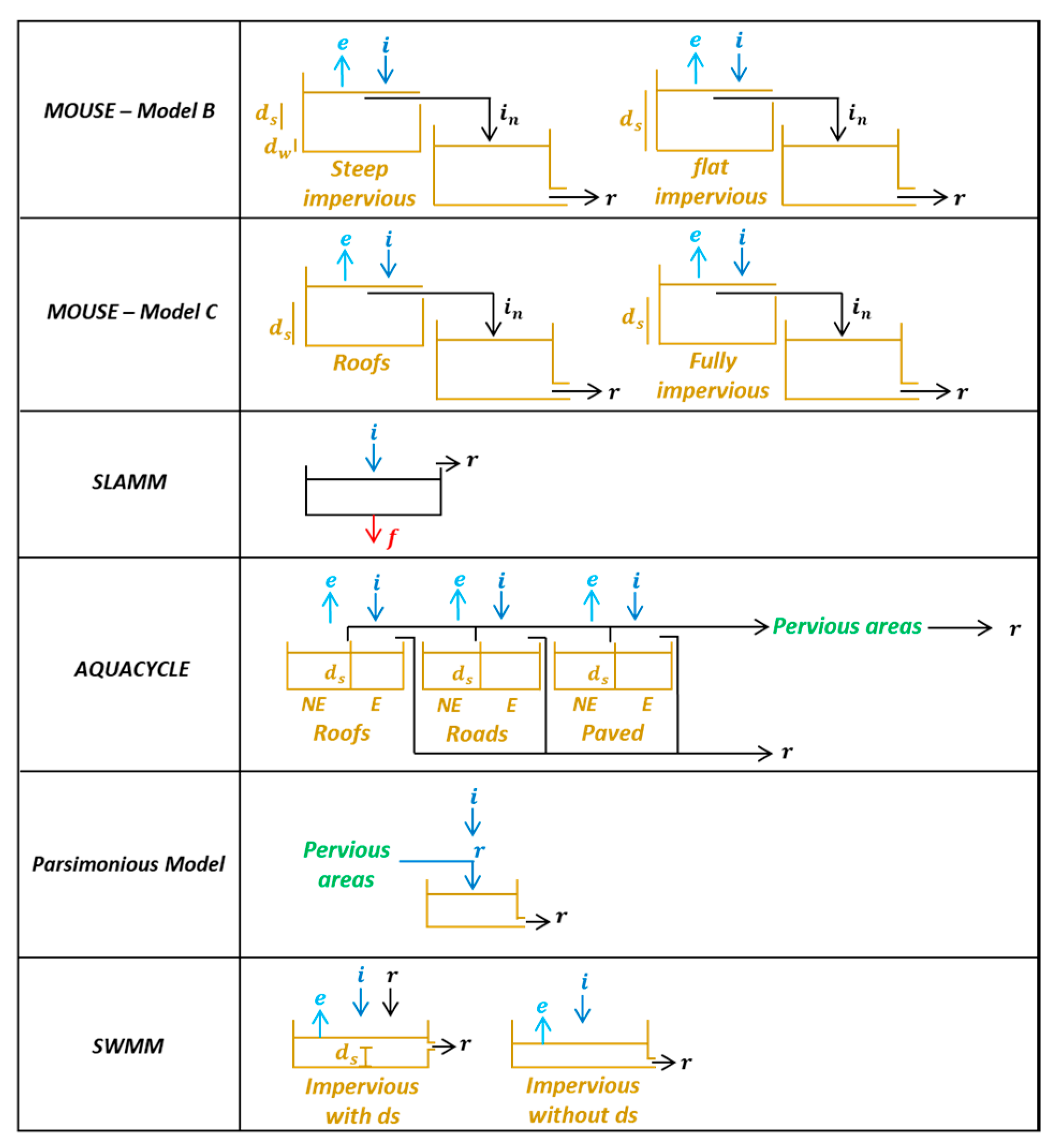
• Initial losses: As described in the previous part of this paper, initial losses refer to two physical quantities: rainfall interception, which is the part of rainfall retained by surface objects and subjected to evaporation process only; and depression storage, which is the part of rainfall retained in surface ponds and is subjected to both evaporation and infiltration. Most hydrological models except for example MOUSE model B (Figure 8) do not make any distinction between these two quantities and hence account for the initial loss using a single parameter representing the maximum storage capacity of surface depressions that once filled will generate surface runoff. This parameter is often supposed to be constant with [12,14] or without [88,89] distinction between different types of land use (Figure 8). However, it is not always taken the same at the beginning of each rainfall event. Some models introduce a temporal variability of this parameter to account for antecedent conditions of each rainfall event [19,84,90] or seasonal effects [83].
• Evaporation: In wet weather conditions, evaporation is theoretically weak and thus has very low contribution to runoff losses. It mainly intervenes after rainfall events to gradually drain the rainfall stock on the catchment surface to restore its retention capacity. A simplified approach is commonly adopted to represent the runoff losses due to evaporation either by directly applying the Potential Evapotranspiration (PET) rate taken to be constant on hourly, daily or monthly scale [14,84,91], or by limiting it by the hydrological state of the surface, more precisely the water depth or the moisture content of the upper surface layer [12,13,90].
• Infiltration: In the hydrological literature, three methods stand out as the most commonly used approaches to model the infiltration process: Curve number, Horton, and Green and Ampt models. Despite the recurrent feedback of the experimental studies in the literature on the significant contribution of infiltration on impervious surfaces, the vast majority of models still assume that infiltration occurs only on pervious areas and neglect it on “impervious” ones. Even in the most detailed representation of the catchment surface tested by [20], the pervious property of paved surfaces identified by on-site observations due to cracks was neglected, leading to overestimation of the other properties (depression storage and manning coefficient) during calibration. Only the fully distributed models (SURF and FullSWOF), the semi-distributed detailed model of [13], and the two lumped models in [19,84] account for the runoff losses on impervious areas due to infiltration. SURF infiltrates rainfall using a modified Horton model, whereas FullSWOF uses modified Green-Ampt formulation. The infiltrated quantity is calculated in [13] with the resolution of the diffusion equation (Richard’s equation) in the porous media of the paved structure. Lumped models developed by [19,84], however, assume infiltration to occur according to a constant rate in time and are only varied according to the surface type. Rodriguez et al. [83] compared the SURF model with and without infiltration on buildings and noticed considerable improvement in the model performance when infiltration capacity on buildings was introduced.

3.2.2. Model Evaluation

Results of model evaluation are summarized in

Table 9. Application and performance evaluation of some fully distributed modeling approaches of rainfall-runoff transformation in urban catchments.

Reference	Model	$\mathit{A}$	${\mathit{C}}_{\mathit{i}\mathit{m}\mathit{p}} (\%)$	Calibration		Validation
				Data	Performance	Data	Performance
[83]	SURF	13.4	39	-	-	7 years	$\mathrm{NSE}\_\mathrm{Q}$ (annual) = 0.77–0.85 $\mathrm{ARE}\_\mathrm{V}$ (annual) = 0.51–31.74%
		4.7	37	1 year	$\mathrm{NSE}\_\mathrm{Q}$ (annual) = 0.77 $\mathrm{ARE}\_\mathrm{V}$ (annual) = 6.5%	6 years	$\mathrm{NSE}\_\mathrm{Q}$ (annual) = 0.68–0.84 $\mathrm{ARE}\_\mathrm{V}$ (annual) = 6.63–27.93%
[104]	FullSWOF	0.2661	-	6 events	$\mathrm{NSE}\_\mathrm{Q}$ (event) = 0.675–0.913	-	-
[93]	Urban Flood model	14109	38	1 event	$\mathrm{ARE}\_\mathrm{V}$ (event) = 6.2%	1 event	$\mathrm{ARE}\_\mathrm{V}$ (event) = 3.9%

for distributed models,

Table 10. Application and performance evaluation of some semi-distributed modeling approaches of rainfall-runoff transformation in urban catchments.

Reference	Model	$\mathit{A}$	${\mathit{C}}_{\mathit{i}\mathit{m}\mathit{p}} (\%)$	Calibration		Validation
				Data	Performance	Data	Performance
[94]	ILLUDAS	0.16–24.68	34–100	2–28 events	$\mathrm{ARE}\_\mathrm{V}$ (event) = 1.9–30.2%	-	-
[11]	Conceptual model (Same parameters were taken for all catchments, optimal values were found to be the same for the four simulated events)	12.8	68	4 events	Graphical evaluations shows good correspondence between hydrographs	-	-
[12]	Aquacycle	445	26	8 years	$\mathrm{NSE}\_\mathrm{Q}$ (daily) = 0.92 $\mathrm{ARE}\_\mathrm{V}$(all) = 0%	9 years	$\mathrm{NSE}\_\mathrm{Q}$ (daily) = 0.94 $\mathrm{ARE}\_\mathrm{V}$ (all) = 8%
		2690	22	8 years	$\mathrm{NSE}\_\mathrm{Q}$ (daily) = 0.96 $\mathrm{ARE}\_\mathrm{V}$ (all) = 0%	5 years	$\mathrm{NSE}\_\mathrm{Q}$ (daily) = 0.90 $\mathrm{ARE}\_\mathrm{V}$ (all) = 5%
[96]	ILSAX	94	24	4 events	$\mathrm{ARE}\_\mathrm{V}$ (event) = 11–150%	2 events	$\mathrm{ARE}\_\mathrm{V}$ (event) = 9–40%
[105]	CANOE (IL ignored, only Cr was calibrated)	3000	40–50	31 events	$\mathrm{NSE}\_\mathrm{V}$ (event) = 0.73	-	-
[13]	Detailed Model	479	100	314 events	$\mathrm{NSE}\_\mathrm{Q}$ (all) = 0.86 $\mathrm{ARE}\_\mathrm{V}$ (all) = 7% ${\mathrm{R}}^2\_\mathrm{Q}$ (event) = 0.87	-	-
		311	100	335 events	$\mathrm{NSE}\_\mathrm{Q}$ (all) = 0.88 $\mathrm{ARE}\_\mathrm{V}$ (all) = 5% ${\mathrm{R}}^2\_\mathrm{Q}$ (event) = 0.88	-	-
[106]	SWMM (Infiltration modeled using Horton equation Kinematic wave model for network flow)	194.9	5	1 event	$\mathrm{NSE}\_\mathrm{Q}$ (event) = 0.25	1 event	$\mathrm{NSE}\_\mathrm{Q}$ (event) = 0.33
		61.8	8	1 event	$\mathrm{NSE}\_\mathrm{Q}$ (event) = 0.80	1 event	$\mathrm{NSE}\_\mathrm{Q}$ (event) = 0.70
		269.8	18	1 event	$\mathrm{NSE}\_\mathrm{Q}$ (event) = 0.75	1 event	$\mathrm{NSE}\_\mathrm{Q}$ (event) = 0.73
		89.5	28	1 event	$\mathrm{NSE}\_\mathrm{Q}$ (event) = 0.77	1 event	$\mathrm{NSE}\_\mathrm{Q}$ (event) = 0.91
		92	37	1 event	$\mathrm{NSE}\_\mathrm{Q}$ (event) = 0.79	1 event	$\mathrm{NSE}\_\mathrm{Q}$ (event) = 0.23
[99]	SWMM	230	-	32 events	$\mathrm{NSE}\_\mathrm{Q}$ (scenario) = 0.79–0.84	22 events	$\mathrm{NSE}\_\mathrm{Q}$ (scenario) = 0.6–0.76
[20]	SWMM (Highest resolution)	5.87	86	6 events	$\mathrm{NSE}\_\mathrm{Q}$ (all) = 0.88 $\mathrm{ARE}\_\mathrm{V}$ (all) = 7%	2 events	$\mathrm{NSE}\_\mathrm{Q}$ (all) = 0.85 $\mathrm{ARE}\_\mathrm{V}$ (all) = 6.5%
		6.63	54	6 events	$\mathrm{NSE}\_\mathrm{Q}$ (all) = 0.97 $\mathrm{ARE}\_\mathrm{V}$ (all) = 9.3%	1 event	$\mathrm{NSE}\_\mathrm{Q}$ (all) = 0.94 $\mathrm{ARE}\_\mathrm{V}$ (all) = 17.8%
	SWMM (Lowest resolution)	5.87	86	6 events	$\mathrm{NSE}\_\mathrm{Q}$ (all) = 0.81 $\mathrm{ARE}\_\mathrm{V}$ (all) = 6.6%	2 events	$\mathrm{NSE}\_\mathrm{Q}$ (all) = 0.83 $\mathrm{ARE}\_\mathrm{V}$ (all) = 2.4%
		6.63	54	6 events	$\mathrm{NSE}\_\mathrm{Q}$ (all) = 0.83 $\mathrm{ARE}\_\mathrm{V}$ (all) = 4.6%	1 event	$\mathrm{NSE}\_\mathrm{Q}$ (all) = 0.86 $\mathrm{ARE}\_\mathrm{V}$ (all) = 8.6%
[107]	SWMM	12.3	39	6 events	$\mathrm{NSE}\_\mathrm{Q}$ (event) = 0.82–0.95 ${\mathrm{R}}^2\_\mathrm{Q}$ (event) = 0.92–0.96	6 events	$\mathrm{NSE}\_\mathrm{Q}$ (event) = 0.90–0.96 ${\mathrm{R}}^2\_\mathrm{Q}$ (event) = 0.84–0.97
						12 events	$\mathrm{NSE}\_\mathrm{Q}$ (event) = 0.41–0.93 ${\mathrm{R}}^2\_\mathrm{Q}$ (event) = 0.78–0.95
[108]	SWMM (Infiltration and evaporation on impervious areas were neglected. Infiltration on pervious areas was modeled using Horton method)	11		1 event	$\mathrm{NSE}\_\mathrm{Q}$ (event) = 0.89	2 events	$\mathrm{NSE}\_\mathrm{Q}$ (event) = 0.8–0.9
[109]	SWMM (Green-Ampt infiltration Dynamic wave for network flow)	11.4	53	3 events	$\mathrm{NSE}\_\mathrm{Q}$ (event) = 0.83–0.93 ${\mathrm{R}}^2\_\mathrm{Q}$ (event) = 0.86–0.93	3 events	$\mathrm{NSE}\_\mathrm{Q}$ (event) = 0.73–0.74 ${\mathrm{R}}^2\_\mathrm{Q}$ (event) = 0.75–0.94
[110]	SWMM (Infiltration modeled using Horton equation Dynamic wave model for network flow)	24.2	69	2 events	$\mathrm{NSE}\_\mathrm{Q}$ (event) = 0.87 ${\mathrm{R}}^2\_\mathrm{Q}$ (event) = 0.86–0.88	1 event	$\mathrm{NSE}\_\mathrm{Q}$ (event) = 0.9 ${\mathrm{R}}^2\_\mathrm{Q}$(event) = 0.95
[111]	SWMM (Green-Ampt for infiltration and dynamic wave for sewer flow. No calibration was realized, parameters were transferred from a similar urban catchment)	33.5	47	-	-	5 events	$\mathrm{NSE}\_\mathrm{Q}$ (event) = 0.76–0.89 $\mathrm{ARE}\_\mathrm{V}$ (event) = 0–31.6 %
[78]	SWMM (lumped + calibration of sub-catchment width and depression storage testing very few values)	0.29	-	39 events	${\mathrm{R}}^2\_\mathrm{Cr}$ (event) = 0.001	-	-
		12	52	13 events	${\mathrm{R}}^2\_\mathrm{Cr}$ (event) = 0	-	-

for semi-distributed models, and

Table 11. Application and performance evaluation of some lumped modeling approaches of rainfall-runoff transformation in urban catchments.

Reference	Model	Surface (ha)	Cimp (%)	Calibration		Validation
				Data	Performance	Data	Performance
[84]	-	4.8	37	361 events	${\mathrm{R}}^2\_\mathrm{Cr}$ (event) = 0.34	405 events	${\mathrm{R}}^2\_\mathrm{Cr}$ (event) = 0.29
	-	4.8	37	361 events	${\mathrm{R}}^2\_\mathrm{Cr}$ (event) = 0.40	405 events	${\mathrm{R}}^2\_\mathrm{Cr}$ (event) = 0.38
[97]	-	177	39	6 events	$\mathrm{NSE}\_\mathrm{Q}$ (event) = 0.55–0.89 $\mathrm{ARE}\_\mathrm{V}$ (event) = 3–11%	-	-
		10.6	40	6 events	$\mathrm{NSE}\_\mathrm{Q}$ (event) = 0.1–0.8 $\mathrm{ARE}\_\mathrm{V}$ (event) = 0–19%	-	-
		155	49	6 events	$\mathrm{NSE}\_\mathrm{Q}$ (event) = 0.4–0.89 $\mathrm{ARE}\_\mathrm{V}$ (event) = 1–28%	-	-
		8.3	98	6 events	$\mathrm{NSE}\_\mathrm{Q}$ (event) = -0.46–0.92 $\mathrm{ARE}\_\mathrm{V}$ (event) = 1–25%	-	-
		25.5	38	6 events	$\mathrm{NSE}\_\mathrm{Q}$ (event) = -10.5–0.97 $\mathrm{ARE}\_\mathrm{V}$ (event) = 6–143%	-	-
		23.6	18	6 events	$\mathrm{NSE}\_\mathrm{Q}$ (event) = 0.26–0.91 $\mathrm{ARE}\_\mathrm{V}$ (event) = 7–34%	-	-
		70	31	6 events	$\mathrm{NSE}\_\mathrm{Q}$ (event) = 0.63–0.91 $\mathrm{ARE}\_\mathrm{V}$ (event) = 1–30%	-	-
[98]	-	0.09 × 10−4	100	49 events $\mathrm{h}$ = 0.1–27	Good visual agreement between simulated and observed cumulative runoff volume	-	-
[19]	-	0.821	75	130 events $\mathrm{h}$ = 0.4-3.7–27 ${\mathrm{I}}_{\max }$ = 0.09–17–360 min-mean-max	$\mathrm{ARE}\_\mathrm{V}$ (event) = 0–257% (>50% for $\mathrm{h}$ < 4 mm)	-	-
[90]	MUSIC	28.2	80	2 years	$\mathrm{NSE}\_\mathrm{Q}$ (all) = 0.54	2 years	$\mathrm{NSE}\_\mathrm{Q}$ (all) = 0.31
		89.1	74		$\mathrm{NSE}\_\mathrm{Q}$ (all) = 0.81		$\mathrm{NSE}\_\mathrm{Q}$ (all) = 0.7
		105.6	51		$\mathrm{NSE}\_\mathrm{Q}$ (all) = 0.62		$\mathrm{NSE}\_\mathrm{Q}$ (all) = 0.32
		38	45		$\mathrm{NSE}\_\mathrm{Q}$ (all) = 0.57		-
		10.5	20		$\mathrm{NSE}\_\mathrm{Q}$ (all) = 0.49		$\mathrm{NSE}\_\mathrm{Q}$ (all) = −0.05
	KAREN	28.2	80	2 years	$\mathrm{NSE}\_\mathrm{Q}$ (all) = 0.53	2 years	$\mathrm{NSE}\_\mathrm{Q}$ (all) = 0.41
		89.1	74		$\mathrm{NSE}\_\mathrm{Q}$ (all) = 0.75		$\mathrm{NSE}\_\mathrm{Q}$ (all) = 0.71
		105.6	51		$\mathrm{NSE}\_\mathrm{Q}$ (all) = 0.63		$\mathrm{NSE}\_\mathrm{Q}$ (all) = 0.39
		38	45		$\mathrm{NSE}\_\mathrm{Q}$ (all) = 0.61		-
		10.5	20		$\mathrm{NSE}\_\mathrm{Q}$ (all) = 0.60		$\mathrm{NSE}\_\mathrm{Q}$ (all) = −1.01

for lumped models. In several modeling attempts, a clear degradation of the runoff flow results was observed when simulating weak rainfall events. A lumped rainfall-runoff model was applied in [19], where results showed that events having a rainfall depth lower than 4 mm recorded more than 50% error on the total runoff volume (Table 11). The application of SWMM on three catchment areas in [20] gave better results for larger events than for smaller events (Table 10). In their investigation of the effect of scale delineation on SWMM parameters and outputs, one of SWMM limitations was identified by [21] in simulating small rain events where both micro- and macro-simulated flow bounds failed to envelope the observations of small rainfall events.

Lumped models seem to offer the least satisfactory performance among the three categories of spatial distribution. This is particularly true when comparing the models’ results on the validation period. The performance of the (semi-)distributed models becomes stable once the model is calibrated, whereas lumped models performance clearly degrades on the validation period. These findings do not, however, imply any correlation between the spatial distribution of the model and its performance, since the fully distributed models show similar or even less satisfactory results than semi-distributed ones for both runoff volume and flow dynamics. Therefore, the degree of spatial distribution necessary to accurately predict the runoff flow is still vague and has incited many researchers to investigate the trade-off between model complexity and performance.

In [20], different configurations of spatial discretization were compared:

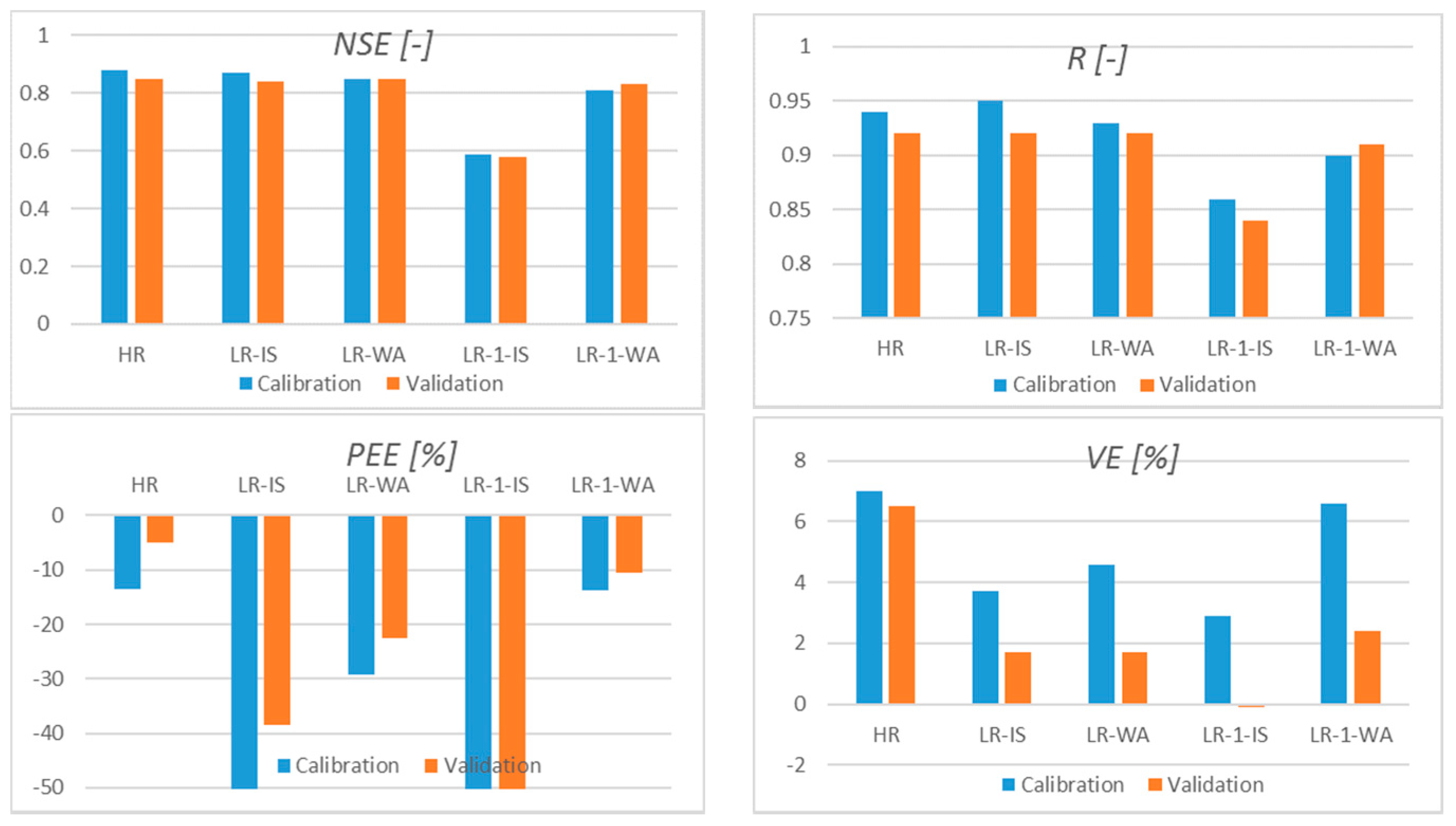
• High-resolution configuration (HR) in which a distinction between all surface types and land uses is made to delineate the sub-catchments that communicate by overland flow before draining to the sewer network, which is fully represented except for the very upstream branches within each sub-catchment.
• Low-resolution configuration (LR-IS) that conserves the definition of sub-catchments of the HR, but without any surface exchange between sub-catchments whose outflow is conveyed directly to the sewer inlet.
• Low-resolution configuration (LR-WA), which lumps all the sub-catchments draining into the same sewer inlet using the weighted average of sub-catchments modeled in the (HR) or (LR-IS) configuration.
• Lowest resolution configuration (LR-1-IS) similar to (LR-IS) but without sewer network
• Lowest resolution configuration (LR-1-WA) similar to (LR-WA) but without the sewer system

The performance metrics: NSE, R, and VE illustrated in Figure 9 for one of the studied catchments indicate a similar or even better performance especially in terms of VE of the LR discretization relative to the HR one. However, the peak error is significantly affected by the change of spatial resolution with the lowest resolution configuration, showing high responsiveness to rainfall and exaggeration in peak flow.

In their investigation of the interest of increasing the quantity of geographical data to parameterize SWMM, Petrucci and Bonhomme [99] tested several scenarios that were all based on the same number of sub-catchments (19 for 2.3 km² catchment area) with some scenarios dividing each sub-catchment into subareas of homogeneous land use and others not. The distinction between the different land uses resulted in a significant improvement in the model performance, eliminating in certain cases the necessity of calibration.

The sensitivity of a conceptual model [11] to the spatial discretization was studied by testing several configurations with different numbers of sub-catchments (32, 18 and 10). Results revealed a very marginal effect on peak values, runoff volume and time to peak. Park et al. [100] evaluated the proper level of spatial resolution for hydrological models using SWMM approach. Findings show that the simulated runoff volume is not affected by perturbations in spatial resolution. Ghosh and Hellweger [101] evaluated the impact of spatial resolution on simulated runoff using SWMM in a 3.7 km² catchment dominated by residential housing. Total outflow volume was relatively insensitive to spatial scale. However, peak flows showed a dual scale effect depending on the storm characteristics. For larger storms, model aggregation reduced peak flows, whereas for smaller storms, aggregation increased peak flows. Stephenson [102] tested whether finer sub-catchments allow closer approximation of the physical model with all parameters being directly measurable. Comparing four levels of spatial discretization, he reported that finely discretized model predicted runoff volumes more accurately than coarse models but that peak flow rates are better predicted by coarser models. Warwick and Litchfield (1993), mentioned in [103], found that aggregation of SWMM did not affect the flow for moderate aggregation, but that lumping to a single sub-catchment altered the flow to an unacceptable degree.

A major advantage of a (semi-)distributed modeling strategy that distinguishes between different surface types is that calibrated values of parameters approach their real physical significance and could be transferred to other similar watersheds. The interest of a semi-distributed model was well proven [20] in this respect when SWMM parameters were calibrated independently on three catchments described with a very high resolution and obtained similar parameter values for same surface types.

Among the semi-distributed ones (Table 10), SWMM is one of the most applied approaches. Like its matches, except ILLUDAS, it produces promising results with NSE values above 0.73, except for very few rainfall events. The best results of the semi-distributed models were obtained by the Aquacycle with NSE values above 0.90 and a relative error on volume not exceeding 8% on the validation period.

Since the performance criteria is generally chosen according to the modeling objective, the modeling attempts reviewed herein having different objectives were evaluated using different criteria, which are not always representative of the runoff loss model performance. The runoff loss model affecting mainly the volume production is best assessed using volume-based criteria. So, when using flow-based criteria, not only the production but also the transfer function is evaluated. So, the better results of NSE_Q obtained for some models cannot be attributed to the runoff loss model but to the combination of both modules: production and transfer. Among the commonly used transfer models, the dynamic wave is the most accurate one accounting for all routing processes (wave translation, backwater effects, wave attenuation, and flow acceleration). However, the kinematic wave model accounting only for wave translation yields less accurate results but is less time consuming. As the routing models have different precision levels, it is hard in the cases when flow-based metrics are used to deduce the quality of runoff loss calculation out of the overall evaluation.

4. Model Parameterization

Rainfall-runoff models involve a certain number of parameters that depend on the structure complexity. A proper application of these models comes to a proper determination of their parameters. In the literature, several methods exist that allow parameterizing these models.

4.1. Reduction of Model Parameters

A common practice when parameterizing a rainfall-runoff model is to reduce the number of model parameters. For that reason, modelers usually conduct a sensitivity analysis to identify the most influential parameters in their model structure, thereby allowing these parameters to be used for calibration. Sensitivity analysis can be broadly divided into local and global approach [112].

A sensitivity analysis was performed in [83] for the 12 parameters of the SURF model to be left finally with seven parameters: the maximum surface storage and concentration time of the three considered surface types: roads, buildings and natural zones, and the saturated permeability that defines the portion of water joining the groundwater. The sensitivity analysis on the CANOE model [105] demonstrated the weak impact of the lag-time parameter used to model overland flow of the discharge hydrograph. This was explained by the small size of sub-catchments used. The reduction of the drainage network, and hence, the sub-catchments discretization increased the model sensitivity to this parameter.

The sensitivity of flow simulations to SWMM parameters has been analyzed and reported in several studies [20,110,113,114]. Barco et al. [113] that both simulated volume and peak flow were most affected by the imperviousness and the surface depression storage. The SWMM model developed by Beling et al. [114] on four peri-urban catchments was highly sensitive to the physical catchment characteristics. The sensitivity analysis conducted by Li et al. [110] on SWMM parameters showed that the depression storage of impervious areas is the most influential parameter when determining the total flow volume, and the roughness coefficient of network system highly affects the total flow and the peak flow. Catchment width was found to be important to accurately simulate peak flow but not the total flow. Results in [20] confirmed those obtained by previous studies regarding the key role of depression storage and imperviousness in predicting the runoff volume using SWMM. Green-Ampt parameters were found to affect the volume of modeled runoff with reasonable limits in highly to moderately urbanized catchments and significantly in weakly urbanized catchment.

For MUSIC and KAREN models, the Effective Impervious Fraction (EIF) seemed to be the most important parameter for runoff prediction [90]. Calibrated values of EIF for both models were found to be significantly lower than the total impervious areas. Ignoring the pervious areas in KAREN model is compensated by higher estimation of effective impervious areas and led to high uncertainties on the EIF calibrated values. MUSIC was considered to be over-parameterized for accounting for the pervious surface contribution to storm-water runoff.

4.2. Using Field Data to Determine Parameter Values

Since all hydrological models involve a certain degree of conceptualism, real physical parameters do not always match those in the model structure, even if both hold the same significance. Model parameters are more “effective” parameters than “real” ones in terms of their representation of the hydrological behavior of the watershed. The more the system representation approaches to reality, the nearer the model parameters get to their real physical values. Therefore, the applicability of the field measurements on the model parameters highly depends on the conceptual degree of the model and its spatial representation of the watershed.

In [99], the benefit of increasing the complexity of the model structure and its spatial distribution was studied in order to include more geographical data in defining the model parameters. Based on the SWMM semi-distributed approach, they tested different levels of GIS data integration in the model structure specifically (1) to determine the impervious cover of each sub-catchment, (2) to define the different land uses on each to be used in decomposing it into further homogeneous sub-catchments, and (3) finally to determine the characteristics of each sub-catchment (hydraulic length and slope). Model performance was found to be insensitive to different scenarios in the calibration phase, but depends on the model structure in validation. Integrating more GIS data in the model structure seemed to improve the model performance in validation but not indefinitely. Results indicated that a certain threshold exists for the benefits obtained from incrementing the use of geographical data. When calibration is possible (i.e., when rainfall and runoff data are available), integrating more geographical data in the model does not necessarily improve its performance. Thus, simpler models would be preferable in this case regarding the reduced efforts it takes to implement them. When calibration is not possible (i.e., when rainfall and runoff data are not available), integrating geographical information in describing the modeled basin provides a good solution to improve the model performance, as it allows to obtain un-calibrated models almost as good as calibrated ones. The geographical information that provides the highest benefit is the land-use classification. However, the optimal level of details to be used in the geographical representation of the modeled system is still not clear.

4.3. Transferring Parameters from Similar Watersheds

When flow measurements are not available, calibration methods cannot be used to determine model parameters. Modelers referred to previous studies to estimate their parameter values e.g., [115]. When a distributed model distinguishing the different types of land covers and uses of a certain catchment area is calibrated, the obtained parameters could be considered as physical characteristics of these surface types, providing, therefore, the option of transferring them to other catchments with similar surface types. In their application of SWMM approach on a 33.5 ha urban catchment, Niemi et al. [111] tested the transferability option of the model parameters from another similar urban catchment calibrated in [20]. For a certain rainfall data source, model performance was acceptable, but parameters were not subjected to a new calibration on the studied catchment to examine the validity of this approach. The same values of the SWMM parameters calibrated in a high-resolution configuration were assigned to the other tested configurations of the same catchment [20], either directly or after calculating their weighted average for the coarser sub-catchments. Also, no verification was made to see whether these parameters could have changed if a new calibration had been conducted. To identify whether fine scale parameterization produces good model results when transported to another catchment, [21] carried out same-scale and cross-scale validation of SWMM parameters calibrated on one urban catchment on another urban catchment in Syracuse (New York). Results showed that parameters derived from the micro-scale delineation accommodate better to the variation in the catchment characteristics, and thus, provide higher confidence level in terms of parameter transferability for modeling other sites than parameters derived from macro-scale delineation.

4.4. Optimization Procedure

Calibration consists of adjusting the model parameters to reduce the error between simulated and observed results. It is one of the most crucial steps of a proper model application [116]. It can be accomplished via manual or automatic procedure. Manual calibration is based on “trial and error” method, whereby parameters are modified in a systematic manner until obtaining the best correlation between the model outputs and observations, as made in [117]. This method is neither practical nor reliable especially when dealing with models characterized by strong non-linearity. It was thus supplanted by automatic techniques developed in a Bayesian framework, like the most used algorithm of Markov Chain Monte Carlo MCMC [118], or in a pseudo-Bayesian framework, like the Genetic Algorithm GA [119,120,121], A MultiALgorithm Genetically Adaptive Multi-objective method AMALGAM [122], the Generalized Likelihood Uncertainty Estimation GLUE [123,124,125,126,127], and the Shuffled Complex Evolution Metropolis Algorithm SCEM-UA [128]. The advantage of these methods is not limited to their reliability and efficiency, but they also provide supplementary information on the uncertainty of the model output and parameter values. However, comparison studies [129,130,131] highlighted the limitations in the assumptions made by these techniques when assessing urban drainage models parameters. SCEM-UA and AMALGAM were found to be quicker than other methods in terms of required number of simulations [131]. All non-Bayesian methods have the subjectivity problem in their acceptance criterion of the parameter sets, while MCMC has a problem with its hypothesis on the normality of residuals.

A challenging aspect of the calibration step is the evaluation of its results. This might be done by visual comparison between observed and simulated hydrographs. However, this method is irreproducible as it relies on subjective judgment [132,133] and cannot be integrated into automatic optimization methods. So, one or more numerical criteria are often used in these algorithms to make objective assessment of the model’s goodness of fit. However, narrowing down the model evaluation to statistical goodness-of-fit metrics makes the model assessment inaccurate and lacks some important aspects of the model performance. A partial representation of the model performance in the optimization criterion leads to what some authors called “equifinality” or “overparameterization” [134,135], i.e., obtaining different sets of optimal parameters that perform equally well on the calibration data but dramatically different when conditions change. Many research efforts are thus being geared in this vein to find the most appropriate and relevant criterion to optimize urban hydrological models. NSE criterion [136] is one of the most commonly used criteria in this context. However, hydrologists have recently pointed out some major limitations and downsides in its formulation and its capacity to represent actual model performance [137,138]. To understand the origin of this defect, Gupta et al. [138] proposed a decomposition of NSE into three components (correlation coefficient $\mathrm{r}$, ratio of standard deviations $\mathsf{\alpha }$, and relative bias $\mathsf{\beta }$) and concluded that optimum NSE is obtained when $\mathsf{\alpha }$ reaches $\mathrm{r}$ rather than 1, which is the real optimum of alpha, implying an underestimation of flow variability. So, a more adequate criterion was proposed therein, the Kling-Gupta criterion (KGE), and is formulated by computing the Euclidian distance of the three components of the NSE criterion from the real optimum.

The calibration procedure becomes trickier when it comes to low flows, since most existing criteria are based on least-square errors that favor the goodness of fit of the hydrograph for high flows and are thus not well adapted to low flows. So, for low-flow simulations, some authors suggested to use common numerical criteria with an appropriate transformation of flow rates to put more emphasis on low values. Houghton-Carr [132] and De Vos et al. [139] used logarithmic transformed flow discharges with mean square error (MSE) criterion to reduce the weight of peak flows. Pechlivanidis et al. [140] and Seeger and Weiler [141] applied the logarithmic transformation to flow discharges in the KGE criterion to fit several rainfall-runoff models on low flows. Beck et al. [142] used the untransformed and log-transformed flows in NSE, R2, and KGE as an evaluation of global models. Montano et al. [143] also used KGE with logarithmic transformation of flow discharges as efficiency measures of the HBV model outputs. In order not to get lost in the jungle of potential alternatives, as called by Pushpalatha et al. [144], some studies were conducted in the literature to compare the efficiency of different indices to evaluate low-flow simulations. Oudin et al. [145] compared several objective functions and concluded that the square root transformation provides an all-purpose efficiency measure. Krause et al. [146] analyzed several calibration indices and found that high flows still contribute in the logarithmic transformation and that a relative efficiency criterion would be the most appropriate objective function to use in a low-flow context. Based on the comparison of nine criteria, Pushpalatha et al. [144] recommended the inverse transformation of flow discharge in NSE criterion to evaluate very low flows. They showed that this transformation would be more adapted than the logarithmic one as it does not show sensitivity to high flow values. Santos et al. [147] showed that logarithmic transformation is not adapted to KGE criterion and might lead to biased evaluation of the model performance.

5. Discussion

In an attempt to understand and redress the weak performance of urban runoff models in representing runoff losses on impervious areas during frequent events, which are essential for urban water quality management, we investigated the most commonly used models and analyzed their structure in light of the latest knowledge on the observed behavior of urban surfaces during storm weather. Many advances were recently made in the literature in the quantification of the relative importance of hydrological processes governing runoff losses in different atmospheric conditions. The experimental assessment of the retention processes affirms that urbanization reduces surface capacity of storing water, but that the order of magnitude of this reduced capacity is still comparable to that of the rainfall depth of frequent events. So, the importance of these retentions might be marginal during heavy events, but for small events and annual scale calculations, they become a key element in conditioning the surface exchange with all the other compartments: with the surface through runoff, with the air through evaporation, and with the soil through infiltration. Both depression storage and rainfall interception are extremely challenging to account for in hydrological modeling due to the high level of heterogeneity characterizing the topography of urban surfaces even on small pavement scale. For that reason, they are usually merged into a single component representing the initial losses on the urban catchments, although the heterogeneity of retention surfaces draws out these processes, undermining the validity of such a practice. Models commonly account for this component by a threshold level for the onset of runoff, which is sometimes separated into two components: interception volume subjected only to evaporation, and depression storage subjected to both infiltration and evaporation.

Hydrologists have for a long time associated urbanization to imperviousness, considering urban cover, especially pavements, as rapid runoff-generators preventing any kind of infiltration. The environmental and safety concerns around urban water management (impact on underground water recharge, pollution of water streams, and increasing flooding risks) driven by this perception incited more research on the hydrological impact of soil sealing. The different direct and indirect techniques used to measure infiltration on paved areas revealed non-negligible rates of infiltration relative to the expected behavior, arguing that paved areas can no more be assumed impervious especially during frequent rainfall events. Field investigations found that the pervious property of paved areas is majorly attributed to infiltration in joints and cracks present on the surface. These observations of infiltration on paved areas are still not integrated in hydrological modeling practice. Aside from the global modeling approaches combining all runoff losses into a single parameter (runoff coefficient) and few detailed approaches, models distinguishing the different runoff losses still do not consider infiltration on paved areas.

Evaporation was also found to be a key process in the hydrological balance of paved areas, accounting for approximately 15% on average of the runoff losses. Its contribution was estimated in different studies on seasonal and annual scale rather than event scale, as it extends on a longer period of time than the event duration. Since this process takes place more in dry weather than wet weather, some modeling approaches supposed it negligible on the event scale. Others used simplified methods to simulate it, either by considering it part of the continuous losses represented by the runoff coefficient or by explicitly taking the minimum between potential evaporation rate and the rainfall depth available on the catchment surface.

A wide panel of urban hydrological models was reviewed in this paper, varying from global to detailed models according to their degree of complexity in representing the hydrological processes and the catchment surface. Global approaches represent the whole catchment as one entity while lumping all hydrological losses taking place. Detailed models, however, involve an explicit way in representing either the hydrological processes or the different surface types. In terms of runoff production on impervious areas, comparison between the two approaches reveals equal degree of simplification in the structure of their production modules. Both approaches have one parameter to represent initial losses (denoted initial loss by global approaches and depression storage by detailed approaches) and another parameter to represent continuous losses (denoted runoff coefficient by global approaches and evaporation and/or infiltration by detailed approaches). A more physical mechanism of infiltration than a constant flux was almost never applied on impervious areas. So, the only difference between the two approaches is the multiplication of these two parameters for the different land uses defined on the studied catchment.

Detailed models were tested in the literature for different levels of spatialization of the catchment surface (lumped, semi-distributed, and totally distributed). When calibrated, both global and detailed approach generate satisfactory results. The choice in this case could not be made in terms of the desired level of precision but in terms of the type of application and sought results. Global approaches are more practical and easy to implement but do not give access to intermediate variables of the repartition of runoff loss neither between different processes nor between different surface types or sub-catchments as in detailed models. Detailed approaches might be preferred when field data for calibration are not available or when the model is to be applied in other temporal and/or spatial conditions. The definition of the most appropriate degree of distribution is, however, more delicate. Detailed modeling seems to be dependent on the spatial distribution, but without showing a strict improvement with the increasing level of discretization, leaving the necessary degree of spatialization vague.

Any hydrological model, whether global or detailed, has some parameters to be determined, a step that constitutes a major concern especially for heterogeneous catchment modeling. Whether field data or calibration procedures are being used, the sensitivity analysis constitutes a primary step to reduce the number of model parameters to be determined. The sensitivity analyses carried out in the literature on detailed hydrological models make a consensus on the determinant property of surface storage on impervious areas or the effective impervious surface in terms of runoff volume, especially when simulating frequent rain events. Using geographical data and physical characteristics to define model parameters depends on the correspondence level between real and modeled representation of the watershed. The geographical data most useful in the model parameterization procedure were found to be the land use classification. Since current hydrological models are still unable to represent watersheds in a perfect faithful manner, many parameters cannot be estimated out of physical characteristics. Calibration techniques become, in this case, inevitable, especially those built in a Bayesian or pseudo-Bayesian framework. Despite their efficient and optimized exploration of the parameters’ space, these methods present certain structural limitations that sometimes question their reliability in optimizing hydrological models.

This review highlights incoherence between our current understanding of the hydrological behavior of urban areas during frequent events and our conception of the production functions in the urban drainage models. Field studies provided more insight into the determinant processes occurring on the different surface types during frequent events, with depression storage being a fundamental element varying between surface types, and for the same surface type and infiltration process, being important on paved areas, especially in their cracks, presenting preferential pathways for rainwater. Integrating this knowledge in hydrological models and finding a way to precisely present the heterogeneity of surface storage should be a priority to improve model performance.

References

1. Hatt, B.E.; Fletcher, T.D.; Walsh, C.J.; Taylor, S.L. The Influence of Urban Density and Drainage Infrastructure on the Concentrations and Loads of Pollutants in Small Streams. Environ. Manag. 2004, 34, 112–124. [Google Scholar] [CrossRef] [PubMed]
2. Walsh, C.J.; Roy, A.H.; Feminella, J.W.; Cottingham, P.D.; Groffman, P.M.; Morgan, R.P. The urban stream syndrome: Current knowledge and the search for a cure. J. N. Am. Benthol. Soc. 2005, 24, 706–723. [Google Scholar] [CrossRef]
3. Niemczynowicz, J. Urban hydrology and water management—Present and future challenges. Urban Water 1999, 1, 1–14. [Google Scholar] [CrossRef]
4. Chocat, B.; Krebs, P.; Marsalek, J.; Rauch, W.; Schilling, W. Urban drainage redefined: From stormwater removal to integrated management. Water Sci. Technol. 2001, 43, 61–68. [Google Scholar] [CrossRef] [PubMed]
5. Chouli, E.; Aftias, E.; Deutsch, J.-C. Applying storm water management in Greek cities: Learning from the European experience. Desalination 2007, 210, 61–68. [Google Scholar] [CrossRef]
6. Fletcher, T.; Andrieu, H.; Hamel, P. Understanding, management and modelling of urban hydrology and its consequences for receiving waters: A state of the art. Adv. Water Resour. 2013, 51, 261–279. [Google Scholar] [CrossRef]
7. Anderson, J.; Iyaduri, R. Integrated urban water planning: Big picture planning is good for the wallet and the environment. Water Sci. Technol. 2003, 47, 19–23. [Google Scholar] [CrossRef]
8. Mitchell, V.G. Applying Integrated Urban Water Management Concepts: A Review of Australian Experience. Environ. Manag. 2006, 37, 589–605. [Google Scholar] [CrossRef]
9. Maheepala, U.; Takyi, A.; Perera, B.J.C. Hydrological data monitoring for urban stormwater drainage systems. J. Hydrol. 2001, 245, 32–47. [Google Scholar] [CrossRef]
10. Beck, N.G.; Conley, G.; Kanner, L.; Mathias, M. An urban runoff model designed to inform stormwater management decisions. J. Environ. Manag. 2017, 193, 257–269. [Google Scholar] [CrossRef]
11. Aronica, G.T.; Cannarozzo, M. Studying the hydrological response of urban catchments using a semi-distributed linear non-linear model. J. Hydrol. 2000, 238, 35–43. [Google Scholar] [CrossRef]
12. Mitchell, V.; Mein, R.; McMahon, T. Modelling the urban water cycle. Environ. Model. Softw. 2001, 16, 615–629. [Google Scholar] [CrossRef]
13. Ramier, D.; Berthier, E.; Andrieu, H. The hydrological behavior of urban streets: Long-term observations and modelling of runoff losses and rainfall-runoff transformation. Hydrol. Process. 2011, 25, 2161–2178. [Google Scholar] [CrossRef]
14. Rossman, L.A. Storm Water Management Model Reference Manual; Volume 1–Hydrology (Revised); EPA: Cincinnati, OH, USA, 2016. [Google Scholar]
15. Hromadka, T. Rainfall-runoff models: A review. Environ. Softw. 1990, 5, 82–103. [Google Scholar] [CrossRef]
16. Zoppou, C. Review of urban storm water models. Environ. Model. Softw. 2001, 16, 195–231. [Google Scholar] [CrossRef]
17. Thorndahl, S.; Schaarup-Jensen, K. Comparative analysis of uncertainties in urban surface runoff modeling. In Proceedings of the International Conference on Sustainable Techniques and Strategies in Urban Water Management, Lyon, France, 25–28 June 2007. [Google Scholar]
18. Berthier, E.; Le Delliou, A.-L. Evaluation of the ‘initial losses—Runoff coefficient’ production function to simulate the usual rain event. In Proceedings of the International Conference on Sustainable Techniques and Strategies in Urban Water Management, Lyon, France, 25–28 June 2007. [Google Scholar]
19. Bressy, A. Flux de micropolluants dans les eaux de ruissellement urbaines: Effets de différents modes de gestion à l’amont. Ph.D. Thesis, Université Paris-Est, Paris, France, 2010. [Google Scholar]
20. Krebs, G.; Kokkonen, T.; Valtanen, M.; Setälä, H.; Koivusalo, H. Spatial resolution considerations for urban hydrological modelling. J. Hydrol. 2014, 512, 482–497. [Google Scholar] [CrossRef]
21. Sun, N.; Hall, M.; Hong, B.; Zhang, L. Impact of SWMM Catchment Discretization: Case Study in Syracuse, New York. J. Hydrol. Eng. 2014, 19, 223–234. [Google Scholar] [CrossRef]
22. Pitt, R.E.; McLean, J. Toronto Area Watershed Management Strategic Study—Humber River Pilot Watershed Project; Ontario Ministry of the Environment: Toronto, ON, Canada, 1986. [Google Scholar]
23. Pandit, A.; Gopalakrishnan, G. Estimation of Annual Storm Runoff Coefficients by Continuous Simulation. J. Irrig. Drain. Eng. 1996, 122, 211–220. [Google Scholar] [CrossRef]
24. Pandit, A.; Gopalakrishnan, G. Estimation of Annual Pollutant Loads under Wet-Weather Conditions. J. Hydrol. Eng. 1997, 2, 211–218. [Google Scholar] [CrossRef]
25. Ramier, D.; Berthier, E.; Andrieu, H. An urban lysimeter to assess runoff losses on asphalt concrete plates. Phys. Chem. EarthParts A/B/C 2004, 29, 839–847. [Google Scholar] [CrossRef]
26. Nehls, T.; Menzel, M.; Wessolek, G. Depression storage capacities of different ideal pavements as quantified by a terrestrial laser scanning-based method. Water Sci. Technol. 2015, 71, 862–869. [Google Scholar] [CrossRef] [PubMed]
27. Redfern, T.W.; Macdonald, N.; Kjeldsen, T.R.; Miller, J.D.; Reynard, N.S. Current understanding of hydrological processes on common urban surfaces. Prog. Phys. Geogr. Earth Environ. 2016, 40, 699–713. [Google Scholar] [CrossRef] [Green Version]
28. Viessman, W., Jr.; Lewis, G.L. Introduction to Hydrology, 4th ed.; Harper Collins: New York, NY, USA, 1996. [Google Scholar]
29. Nakayoshi, M.; Moriwaki, R.; Kawai, T.; Kanda, M. Experimental study on rainfall interception over an outdoor urban-scale model. Water Resour. Res. 2009, 45, W04415. [Google Scholar] [CrossRef] [Green Version]
30. Davies, H.A. The Water Balance of Urban Impermeable Surfaces Catchment and Process Studies. Ph.D. Thesis, University College London, London, UK, 1981. [Google Scholar]
31. Ragab, R.; Bromley, J.; Rosier, P.; Cooper, J.D.; Gash, J.H.C. Experimental study of water fluxes in a residential area: 1. Rainfall, roof runoff and evaporation: The effect of slope and aspect. Hydrol. Process. 2003, 17, 2409–2422. [Google Scholar] [CrossRef]
32. Farreny, R.; Morales-Pinzón, T.; Guisasola, A.; Tayà, C.; Rieradevall, J.; Gabarrell, X. Roof selection for rainwater harvesting: Quantity and quality assessments in Spain. Water Res. 2011, 45, 3245–3254. [Google Scholar] [CrossRef] [PubMed]
33. Asadian, Y.; Weiler, M. A New Approach in Measuring Rainfall Interception by Urban Trees in Coastal British Columbia. Water Qual. Res. J. 2009, 44, 16–25. [Google Scholar] [CrossRef]
34. David, T.S.; Gash, J.H.C.; Valente, F.; Pereira, J.S.; Ferreira, M.I.; David, J.S.; Ferreira, M. Rainfall interception by an isolated evergreen oak tree in a Mediterranean savannah. Hydrol. Process. 2006, 20, 2713–2726. [Google Scholar] [CrossRef]
35. Guevara-Escobar, A.; Gonzalez-Sosa, E.; Véliz-Chávez, C.; Ventura-Ramos, E.; Ramos-Salinas, M. Rainfall interception and distribution patterns of gross precipitation around an isolated Ficus benjamina tree in an urban area. J. Hydrol. 2007, 333, 532–541. [Google Scholar] [CrossRef]
36. Inkiläinen, E.N.; McHale, M.R.; Blank, G.B.; James, A.; Nikinmaa, E. The role of the residential urban forest in regulating throughfall: A case study in Raleigh, North Carolina, USA. Landsc. Urban Plan. 2013, 119, 91–103. [Google Scholar] [CrossRef]
37. Xiao, Q.; McPherson, E.G.; Ustin, S.L.; Grismer, M.E.; Simpson, J.R. Winter rainfall interception by two mature open-grown trees in Davis, California. Hydrol. Process. 2000, 14, 763–784. [Google Scholar] [CrossRef]
38. Li, X.; Xiao, Q.; Niu, J.; Dymond, S.; Van Doorn, N.S.; Yu, X.; Xie, B.; Lv, X.; Zhang, K.; Li, J. Process-based rainfall interception by small trees in Northern China: The effect of rainfall traits and crown structure characteristics. Agric. Meteorol. 2016, 218–219, 65–73. [Google Scholar] [CrossRef]
39. Xiao, Q.; McPherson, G.E. Surface Water Storage Capacity of Twenty Tree Species in Davis, California. J. Environ. Qual. 2016, 45, 188–198. [Google Scholar] [CrossRef] [PubMed]
40. Hollis, G.E.; Ovenden, J.C. One year irrigation experiment to assess losses and runoff volume relationships for a residential road in hertfordshire, England. Hydrol. Process. 1988, 2, 61–74. [Google Scholar] [CrossRef]
41. Marsalek, J.; Jiménez-Cisneros, B.E.; Malmquist, P.-A.; Karamouz, M.; Goldenfum, J.; Chocat, B. Urban Water Cycle Processes and Interactions. In Urban Water Cycle Processes and Interactions; Informa UK Limited: Colchester, UK, 2014. [Google Scholar]
42. Llorens, P.; Poch, R.; Latron, J.; Gallart, F. Rainfall interception by a Pinus sylvestris forest patch overgrown in a Mediterranean mountainous abandoned area I. Monitoring design and results down to the event scale. J. Hydrol. 1997, 199, 331–345. [Google Scholar] [CrossRef]
43. Llorens, P.; Domingo, F. Rainfall partitioning by vegetation under Mediterranean conditions. A review of studies in Europe. J. Hydrol. 2007, 335, 37–54. [Google Scholar] [CrossRef]
44. Xiao, Q.; McPherson, E.G. Rainfall interception by Santa Monica’s municipal urban forest. Urban Ecosyst. 2002, 6, 291–302. [Google Scholar] [CrossRef]
45. Wang, J.; Endreny, T.A.; Nowak, D.J. Mechanistic Simulation of Tree Effects in an Urban Water Balance Model1. Jawra J. Am. Water Resour. Assoc. 2008, 44, 75–85. [Google Scholar] [CrossRef]
46. Armson, D.; Stringer, P.; Ennos, A. The effect of street trees and amenity grass on urban surface water runoff in Manchester, UK. Urban For. Urban Green. 2013, 12, 282–286. [Google Scholar] [CrossRef]
47. Livesley, S.J.; Baudinette, B.; Glover, D. Rainfall interception and stem flow by eucalypt street trees—The impacts of canopy density and bark type. Urban For. Urban Green. 2014, 13, 192–197. [Google Scholar] [CrossRef]
48. Salvadore, E.; Bronders, J.; Batelaan, O.; Elga, S.; Jan, B.; Okke, B. Hydrological modelling of urbanized catchments: A review and future directions. J. Hydrol. 2015, 529, 62–81. [Google Scholar] [CrossRef]
49. Mansell, M.; Rollet, F. Water balance and the behaviour of different paving surfaces. Water Environ. J. 2006, 20, 7–10. [Google Scholar] [CrossRef]
50. Pandit, A.; Heck, H.H. Estimations of Soil Conservation Service Curve Numbers for Concrete and Asphalt. J. Hydrol. Eng. 2009, 14, 335–345. [Google Scholar] [CrossRef]
51. Wiles, T.J.; Sharp, J.J.M. The Secondary Permeability of Impervious Cover. Environ. Eng. Geosci. 2008, 14, 251–265. [Google Scholar] [CrossRef]
52. Ragab, R.; Rosier, P.; Dixon, A.; Bromley, J.; Cooper, J.D. Experimental study of water fluxes in a residential area: 2. Road infiltration, runoff and evaporation. Hydrol. Process. 2003, 17, 2423–2437. [Google Scholar] [CrossRef]
53. Raimbault, G. Cycles annuels d’humidité dans une chaussée souple et son support. Bull. Liaison Lab. Ponts Chaussées 1986, 145, 79–84. [Google Scholar]
54. Raimbault, G.; Silvestre, P. Analyse des variations d’état hydrique dans les chaussées. Bull. Liaison Lab. Ponts Chaussées 1990, 238, 39–50. [Google Scholar]
55. Ramier, D. Water Balance on Urban Roads: Observations and Modeling. Ph.D. Thesis, Ecole Centrale de Nantes, Nantes University, Nantes, France, 2005. [Google Scholar]
56. Letellier, L.; Berthier, E.; Dabroux, N. Développement d’un infiltromètre pour mesurer les infiltrations d’eau à la surface des chaussées. Bulletin des Lab. des Ponts et Chaussées 2010, 277, 19–30. [Google Scholar]
57. Illgen, M. Infiltration and surface runoff processes on pavements: Physical phenomena and modelling. In Proceedings of the 11th International Conference on Urban Drainage, Edinburgh, Scotland, UK, 31 August–5 September 2008. [Google Scholar]
58. Zondervan, J.G. Modelling Urban Runoff—A Quasi-Linear Approach. Ph.D. Thesis, Wageningen University and Research, Wageningen, The Netherlands, 1978. [Google Scholar]
59. SETRA-LCPC. Guide technique. In Écrans Drainants en Rives de Chaussées; SETRA: Bagneux, France, 1992; p. 71. [Google Scholar]
60. Raimbault, G.; Andrieu, H.; Berthier, E.; Joannis, C.; Legret, M. Infiltration des eaux pluviales à travers les surfaces urbaines: Des revêtements imperméables aux structures-réservoirs. Bull. Liaison Lab. Ponts Chaussées 2002, 167, 77–84. [Google Scholar]
61. Cooley, L.A., Jr.; Brown, E.R.; Maghsoodloo, S. Developing critical field permeability and pavement density values for coarse—Graded superpave pavements. J. Transport. Res. Board 2001, 1761, 1–3. [Google Scholar] [CrossRef]
62. Vivar, E.; Haddock, J.E. Hot-mix asphalt permeability and porosity. J. Assoc. Asph. Paving Technol. 2007, 76, 953–979. [Google Scholar]
63. Huang, B.; Mohammad, L.N.; Raghavendra, A.; Abadie, C. Fundamentals of permeability in asphalt mixtures. In Report of the Annual Meeting of the Association of Asphalt Paving Technologist; AAPT: Chicago, IL, USA, 1999. [Google Scholar]
64. Borgwardt, S. In-situ infiltration performance of permeable concrete block pavement—New results. In Proceedings of the 11th International Conference on Concrete Block Pavement—ICCBP, Dresden, Germany, 8–11 September 2015. [Google Scholar]
65. Ridgeway, H.H. Infiltration of water through the pavement surface. In Transportation Research Record; Transport Research Board: Washington, DC, USA, 1976; p. 616. [Google Scholar]
66. Cheng, L.; Xu, Z.; Wang, D.; Cai, X. Assessing interannual variability of evapotranspiration at the catchment scale using satellite-based evapotranspiration data sets. Water Resour. Res. 2011, 47, W09509. [Google Scholar] [CrossRef] [Green Version]
67. Timm, A.; Kluge, B.; Wessolek, G. Hydrological balance of paved surfaces in moist mid-latitude climate—A review. Landsc. Urban Plan. 2018, 175, 80–91. [Google Scholar] [CrossRef]
68. Cohard, J.-M.; Rosant, J.-M.; Rodriguez, F.; Andrieu, H.; Mestayer, P.G.; Guillevic, P. Energy and water budgets of asphalt concrete pavement under simulated rain events. Urban Clim. 2018, 24, 675–691. [Google Scholar] [CrossRef]
69. Boyd, M.J.; Bufill, M.C.; Knee, R.M. Pervious and impervious runoff in urban catchments. Hydrol. Sci. J. 1993, 38, 463–478. [Google Scholar] [CrossRef]
70. Dayaratne, S.T.; Perera, B.J.C. Regionalization of impervious area parameters of urban drainage models. Urban Water J. 2008, 5, 231–246. [Google Scholar] [CrossRef]
71. Kidd, C.H.R. Rainfall-runoff processes over urban surfaces. In Proceedings of the International Urban Hydrology Workshop, Institute of Hydrology, Wallingford, UK, April 1978. [Google Scholar]
72. HR Wallingford. Wallingford Procedure for Design and Analysis of Urban Storm Drainage; HR Wallingford: Wallingford, UK, 1983. [Google Scholar]
73. Pratt, C.J.; Harrison, J.J. Development and assessment of a runoff simulation model for Clifton Grove catchment. In Proceedings of the Urban Drainage Modelling, Dubrovnik, Croatia, 8–11 April 1986; Pergamon Press: London, UK, 1986; pp. 293–303. [Google Scholar]
74. Bertrand-Krajewski, J.L. Urban Hydrology Course, Part 3: Losses before runoff; INSA de Lyon: Lyon, France, 2006. [Google Scholar]
75. Chocat, B.; Thibault, S.; Seguin, D. Hydrologie Urbaine et Assainissement; Cours de l’INSA de Lyon: Lyon, France, 1982; Tome 1. [Google Scholar]
76. Jovanovic, S. Hydrologic approaches in urban drainage system modelling. In Urban Drainage Modelling; Pergamon Press: London, UK, 1986; pp. 185–208. [Google Scholar]
77. Rim, Y.-N. Analyzing Runoff Dynamics of Paved Soil Surface Using Weighable Lysimeters. Ph.D. Thesis, Technical University of Berlin, Berlin, Germany, 2017. [Google Scholar]
78. Alhoujayri, M. Evaluation of Production Functions of Runoff during Frequent Rainfall Events. Master’s Thesis, Lebanese University, Hadat, Lebanon, 2017. [Google Scholar]
79. Pitt, R.E. Small Storm Urban Flow and Particulate Washoff Contributions to Outfall Discharges. Ph.D. Thesis, University of Wisconsin-Madison, Madison, WI, USA, 1987. [Google Scholar]
80. Brulé, D.; Blanchet, F.; Rousselle, J. Study of runoff losses on impervious surfaces in an urban environment. J. Water Sci. 1997, 10, 147–166. [Google Scholar]
81. Chocat, B. Notice Canoe—Version 3; INSA Lyon-Sogreah-Alison: Villeurban, France, 2014. [Google Scholar]
82. Mosini, M.-L.; Rodriguez, F.; Andrieu, H. Statistical Properties of The Hydrological Response of a Small-Urbanized Watershed: Application on the Experimental Site of Rezé; Technical Note of Laboratoire des Ponts et Chaussées; LCPC: Paris, France, 2000; pp. 105–110. [Google Scholar]
83. Rodriguez, F.; Andrieu, H.; Zech, Y. Evaluation of a distributed model for urban catchments using a 7-year continuous data series. Hydrol. Process. 2000, 14, 899–914. [Google Scholar] [CrossRef]
84. Berthier, E.; Rodriguez, F.; Andrieu, H.; Raimbault, G. The limits of the model of initial loss and runoff coefficient when simulating frequent rainfall events. In Proceedings of the International Conference on Sustainable Techniques and Strategies in Urban Water Management, Lyon, France, 25–27 June 2001. (In French). [Google Scholar]
85. Thorndahl, S.; Johansen, C.; Schaarup-Jensen, K. Assessment of runoff contributing catchment areas in rainfall runoff modelling. Water Sci. Technol. 2006, 54, 49–56. [Google Scholar] [CrossRef]
86. Sun, S.; Barraud, S.; Branger, F.; Braud, I.; Castebrunet, H. Urban hydrologic trend analysis based on rainfall and runoff data analysis and conceptual model calibration. Hydrol. Process. 2017, 31, 1349–1359. [Google Scholar] [CrossRef] [Green Version]
87. Liaw, C.-H.; Tsai, Y.-L. Optimum storage volume of rooftop rainwater harvesting systems for domestic use. J. Am. Water Resour. Assoc. 2004, 40, 901–912. [Google Scholar] [CrossRef]
88. Pitt, R.E. University of Alabama Unique Features of the Source Loading and Management Model (SLAMM). J. Water Manag. Model. 1998, 6, 13–35. [Google Scholar] [CrossRef] [Green Version]
89. Coutu, S.; Del Giudice, D.; Rossi, L.; Barry, D.A. Parsimonious hydrological modeling of urban sewer and river catchments. J. Hydrol. 2012, 464–465, 477–484. [Google Scholar] [CrossRef] [Green Version]
90. Dotto, C.B.S.; Kleidorfer, M.; Deletic, A.; Rauch, W.; McCarthy, D.; Fletcher, T. Performance and sensitivity analysis of stormwater models using a Bayesian approach and long-term high resolution data. Environ. Model. Softw. 2011, 26, 1225–1239. [Google Scholar] [CrossRef]
91. Bellal, M.; Sillen, X.; Zech, Y. Coupling GIS with a distributed hydrological model for studying the effect of various urban planning options on rainfall-runoff relationship in urbanized watersheds. In Proceedings of the Hydrology’s 96 Conference, Vienna, Austria, 16–19 April 1996; pp. 99–106. [Google Scholar]
92. Delestre, O.; Cordier, S.; Darboux, F.; Du, M.; James, F.; Laguerre, C.; Lucas, C.; Planchon, O. FullSWOF: A Software for Overland Flow Simulation. In Springer Water; Gourbesville, P., Cunge, J., Caignaert, G., Eds.; Springer Science and Business Media LLC: Berlin/Heidelberg, Germany, 2013; pp. 221–231. [Google Scholar]
93. Liu, J.; Shao, W.; Xiang, C.; Mei, C.; Li, Z. Uncertainties of urban flood modeling: Influence of parameters for different underlying surfaces. Environ. Res. 2020, 182, 108929. [Google Scholar] [CrossRef] [PubMed]
94. Terstriep, M.L.; Stall, J.B. The Illinois Urban Drainage Area Simulator: ILLUDAS; Bulletin no. 58; Illinois State Water Survey: Champaign, IL, USA, 1974. [Google Scholar]
95. Mitchell, V.; Diaper, C. Simulating the urban water and contaminant cycle. Environ. Model. Softw. 2006, 21, 129–134. [Google Scholar] [CrossRef]
96. Dayaratne, S.T.; Perera, B.J.C. Calibration of urban stormwater drainage models using hydrograph modelling. Urban Water J. 2004, 1, 283–297. [Google Scholar] [CrossRef] [Green Version]
97. Bernadotte, G. La méthode rationnelle généralisée: Analyse de sensibilité et performance du modèle. Master’s Thesis, Ecole de Technologie supérieure, Montréal, QC, Canada, 2006. [Google Scholar]
98. Mansell, M.; Rollet, F. The effect of surface texture on evaporation, infiltration and storage properties of paved surfaces. Water Sci. Technol. 2009, 60, 71–76. [Google Scholar] [CrossRef]
99. Petrucci, G.; Bonhomme, C. The dilemma of spatial representation for urban hydrology semi-distributed modelling: Trade-offs among complexity, calibration and geographical data. J. Hydrol. 2014, 517, 997–1007. [Google Scholar] [CrossRef]
100. Park, S.Y.; Lee, K.W.; Park, I.H.; Ha, S.R. Effect of the aggregation level of surface runoff fields and sewer network for a SWMM simulation. Desalination 2008, 226, 328–337. [Google Scholar] [CrossRef]
101. Ghosh, I.; Hellweger, F. Effects of Spatial Resolution in Urban Hydrologic Simulations. J. Hydrol. Eng. 2012, 17, 129–137. [Google Scholar] [CrossRef] [Green Version]
102. Stephenson, D. Selection of Stormwater Model Parameters. J. Environ. Eng. 1989, 115, 210–220. [Google Scholar] [CrossRef]
103. Elliott, A.H.; Trowsdale, S.; Wadhwa, S. Effect of Aggregation of On-Site Storm-Water Control Devices in an Urban Catchment Model. J. Hydrol. Eng. 2009, 14, 975–983. [Google Scholar] [CrossRef]
104. Hong, Y.; Bonhomme, C.; Le, M.-H.; Chebbo, G. A new approach of monitoring and physically-based modelling to investigate urban wash-off process on a road catchment near Paris. Water Res. 2016, 102, 96–108. [Google Scholar] [CrossRef] [PubMed]
105. Lhomme, J.; Bouvier, C.; Perrin, J.-L. Applying a GIS-based geomorphological routing model in urban catchments. J. Hydrol. 2004, 299, 203–2016. [Google Scholar] [CrossRef]
106. Wu, J.Y.; Thompson, J.R.; Kolka, R.K.; Franz, K.J.; Stewart, T.W. Using the Storm Water Management Model to predict urban headwater stream hydrological response to climate and land cover change. Hydrol. Earth Syst. Sci. 2013, 17, 4743–4758. [Google Scholar] [CrossRef] [Green Version]
107. Guan, M.; Sillanpää, N.; Koivusalo, H. Modelling and assessment of hydrological changes in a developing urban catchment. Hydrol. Process. 2015, 29, 2880–2894. [Google Scholar] [CrossRef]
108. Yao, L.; Chen, L.; Wei, W. Assessing the effectiveness of imperviousness on stormwater runoff in micro urban catchments by model simulation. Hydrol. Process. 2015, 30, 1836–1848. [Google Scholar] [CrossRef] [Green Version]
109. Raudaskoski, O. Modelling Urban Stormwater Management Alternatives. Master’s Thesis, Aalto University, School of Engineering, Espoo, Finland, 2016. [Google Scholar]
110. Li, C.; Liu, M.; Hu, Y.; Gong, J.; Xu, Y. Modeling the Quality and Quantity of Runoff in a Highly Urbanized Catchment Using Storm Water Management Model. Pol. J. Environ. Stud. 2016, 25, 1573–1581. [Google Scholar] [CrossRef]
111. Niemi, T.; Warsta, L.; Taka, M.; Hickman, B.; Pulkkinen, S.; Krebs, G.; Moisseev, D.; Koivusalo, H.; Kokkonen, T. Applicability of open rainfall data to event-scale urban rainfall-runoff modelling. J. Hydrol. 2017, 547, 143–155. [Google Scholar] [CrossRef] [Green Version]
112. Saltelli, A.; Tarantola, S.; Campolongo, F. Sensitivity analysis as an ingredient of modeling. Stat. Sci. 2000, 15, 377–395. [Google Scholar]
113. Barco, J.; Wong, K.M.; Stenstrom, M.K. Automatic Calibration of the U.S. EPA SWMM Model for a Large Urban Catchment. J. Hydraul. Eng. 2008, 134, 466–474. [Google Scholar] [CrossRef]
114. Beling, F.A.; Garcia, J.I.B.; Paiva, E.M.C.D.; Bastos, G.A.P.; Paiva, J.B.D. Analysis of the SWMM model parameters for runoff evaluation in periurban basins from southern Brazil. In Proceedings of the 12th International Conference on Urban Drainage (iCUD), Porto Alegre, Brazil, 11–16 September 2011; pp. 1–8. [Google Scholar]
115. Kourtis, I.M.; Tsihrintzis, V.A.; Baltas, E. Simulation of Low Impact Development (LID) Practices and Comparison with Conventional Drainage Solutions. Proceedings 2018, 2, 640. [Google Scholar] [CrossRef] [Green Version]
116. Dendrou, S.A. Overview of Urban Stormwater Models. Water Resour. Monogr. 2013, 219–247. [Google Scholar] [CrossRef]
117. Rosa, D.J.; Clausen, J.C.; Dietz, M.E. Calibration and Verification of SWMM for Low Impact Development. Jawra J. Am. Water Resour. Assoc. 2015, 51, 746–757. [Google Scholar] [CrossRef]
118. Dotto, C.B.S.; Deletic, A.; McCarthy, D.; Fletcher, T.D. Calibration and Sensitivity Analysis of Urban Drainage Models: Music Rainfall/Runoff Module and a Simple Stormwater Quality Model. Australas. J. Water Resour. 2011, 15, 85–94. [Google Scholar] [CrossRef]
119. Liong, S.-Y.; Chan, W.T.; Shreeram, J. Peak-Flow Forecasting with Genetic Algorithm and SWMM. J. Hydraul. Eng. 1995, 121, 613–617. [Google Scholar] [CrossRef]
120. Cai, X.; McKinney, D.C.; Lasdon, L.S. Solving nonlinear water management models using a combined genetic algorithm and linear programming approach. Adv. Water Resour. 2001, 24, 667–676. [Google Scholar] [CrossRef]
121. Khu, S.-T.; Di Pierro, F.; Savić, D.; Djordjevic, S.; Walters, G. Incorporating spatial and temporal information for urban drainage model calibration: An approach using preference ordering genetic algorithm. Adv. Water Resour. 2006, 29, 1168–1181. [Google Scholar] [CrossRef]
122. Vrugt, J.A.; Robinson, B.A. Improved evolutionary optimization from genetically adaptive multimethod search. Proc. Natl. Acad. Sci. USA 2007, 104, 708–711. [Google Scholar] [CrossRef] [PubMed] [Green Version]
123. Beven, K.; Binley, A. The future of distributed models: Model calibration and uncertainty prediction. Hydrol. Process. 1992, 6, 279–298. [Google Scholar] [CrossRef]
124. Beven, K.; Freer, J. Equifinality, data assimilation, and uncertainty estimation in mechanistic modelling of complex environmental systems using the GLUE methodology. J. Hydrol. 2001, 249, 11–29. [Google Scholar] [CrossRef]
125. Mannina, G.; Freni, G.; Viviani, G.; Sægrov, S.; Hafskjold, L. Integrated urban water modelling with uncertainty analysis. Water Sci. Technol. 2006, 54, 379–386. [Google Scholar] [CrossRef] [PubMed]
126. Thorndahl, S.; Beven, K.; Jensen, J.; Schaarup-Jensen, K. Event based uncertainty assessment in urban drainage modelling, applying the GLUE methodology. J. Hydrol. 2008, 357, 421–437. [Google Scholar] [CrossRef] [Green Version]
127. Freni, G.; Mannina, G.; Viviani, G.; Viviani, G. Uncertainty in urban stormwater quality modelling: The influence of likelihood measure formulation in the GLUE methodology. Sci. Total Environ. 2009, 408, 138–145. [Google Scholar] [CrossRef]
128. Vrugt, J.A.; Gupta, H.V.; Bouten, W.; Sorooshian, S. A Shuffled Complex Evolution Metropolis algorithm for optimization and uncertainty assessment of hydrologic model parameters. Water Resour. Res. 2003, 39, 11–116. [Google Scholar] [CrossRef] [Green Version]
129. Makowski, D.; Wallach, D.; Tremblay, M. Using a Bayesian approach to parameter estimation; comparison of the GLUE and MCMC methods. Agronomie 2002, 22, 191–203. [Google Scholar] [CrossRef]
130. Freni, G.; Mannina, G.; Viviani, G. Urban runoff modelling uncertainty: Comparison among Bayesian and pseudo-Bayesian methods. Environ. Model. Softw. 2009, 24, 1100–1111. [Google Scholar] [CrossRef]
131. Dotto, C.B.S.; Mannina, G.; Kleidorfer, M.; Vezzaro, L.; Henrichs, M.; McCarthy, D.; Freni, G.; Rauch, W.; Deletic, A. Comparison of different uncertainty techniques in urban stormwater quantity and quality modelling. Water Res. 2012, 46, 2545–2558. [Google Scholar] [CrossRef]
132. Houghton-Carr, H.A. Assessment criteria for simple conceptual daily rainfall-runoff models. Hydrol. Sci. J. 1999, 44, 237–261. [Google Scholar] [CrossRef]
133. Crochemore, L.; Perrin, C.; Andréassian, V.; Ehret, U.; Seibert, S.P.; Grimaldi, S.; Gupta, H.V.; Paturel, J.-E.; Grimaldi, S. Comparing expert judgement and numerical criteria for hydrograph evaluation. Hydrol. Sci. J. 2015, 60, 402–423. [Google Scholar] [CrossRef]
134. Gupta, V.K.; Sorooshian, S. Uniqueness and observability of conceptual rainfall-runoff model parameters: The percolation process examined. Water Resour. Res. 1983, 19, 269–276. [Google Scholar] [CrossRef]
135. Beven, K. Prophecy, reality and uncertainty in distributed hydrological modelling. Adv. Water Resour. 1993, 16, 41–51. [Google Scholar] [CrossRef]
136. Nash, J.E.; Sutcliffe, J.V. River Flow forecasting through conceptual models-Part I: A discussion of principles. J. Hydrol. 1970, 10, 282–290. [Google Scholar] [CrossRef]
137. Jain, S.K.; Sudheer, K.P. Fitting of Hydrologic Models: A Close Look at the Nash–Sutcliffe Index. J. Hydrol. Eng. 2008, 13, 981–986. [Google Scholar] [CrossRef]
138. Gupta, H.V.; Kling, H.; Yilmaz, K.K.; Martinez, G.F. Decomposition of the mean squared error and NSE performance criteria: Implications for improving hydrological modelling. J. Hydrol. 2009, 377, 80–91. [Google Scholar] [CrossRef] [Green Version]
139. De Vos, N.J.; Rientjes, T.H.M.; Gupta, H.V. Diagnostic evaluation of conceptual rainfall-runoff models using temporal clustering. Hydrol. Process. 2010, 24, 2840–2850. [Google Scholar] [CrossRef]
140. Pechlivanidis, I.; Jackson, B.; McMillan, H.; Gupta, H. Use of an entropy-based metric in multiobjective calibration to improve model performance. Water Resour. Res. 2014, 50, 8066–8083. [Google Scholar] [CrossRef]
141. Seeger, S.; Weiler, M. Reevaluation of transit time distributions, mean transit times and their relation to catchment topography. Hydrol. Earth Syst. Sci. 2014, 18, 4751–4771. [Google Scholar] [CrossRef] [Green Version]
142. Beck, H.E.; Van Dijk, A.I.J.M.; De Roo, A.; Miralles, D.G.; McVicar, T.R.; Schellekens, J.; Bruijnzeel, L.A. Global-scale regionalization of hydrologic model parameters. Water Resour. Res. 2016, 52, 3599–3622. [Google Scholar] [CrossRef] [Green Version]
143. Montano, B.Q.; Westerberg, I.K.; Fuentes-Andino, D.; Hidalgo, H.G.; Halldin, S. Can climate variability information constrain a hydrological model for an ungauged Costa Rican catchment? Hydrol. Process. 2018, 32, 830–846. [Google Scholar] [CrossRef]
144. Pushpalatha, R.; Perrin, C.; Le Moine, N.; Andréassian, V. A review of efficiency criteria suitable for evaluating low-flow simulations. J. Hydrol. 2012, 420, 171–182. [Google Scholar] [CrossRef]
145. Oudin, L.; Andréassian, V.; Mathevet, T.; Perrin, C.; Michel, C. Dynamic averaging of rainfall-runoff model simulations from complementary model parameterizations. Water Resour. Res. 2006, 42. [Google Scholar] [CrossRef]
146. Krause, P.; Boyle, D.P.; Bäse, F. Comparison of different efficiency criteria for hydrological model assessment. Adv. Geosci. 2005, 5, 89–97. [Google Scholar] [CrossRef] [Green Version]
147. Santos, L.; Thirel, G.; Perrin, C. Technical note: Pitfalls in using log-transformed flows within the KGE criterion. Hydrol. Earth Syst. Sci. 2018, 22, 4583–4591. [Google Scholar] [CrossRef] [Green Version]
Figure 1. Diagram of physical processes governing runoff production in urban areas.
Water 12 02777 g001
Figure 2. Temporal variation of the infiltration rate of paved areas during an irrigation experiment (Extract from [47]).
Water 12 02777 g002
Figure 3. Temporal variation of the infiltration rate of paved surface measured using a double-ring infiltrometer (Extract from [56]).
Water 12 02777 g003
Figure 4. Measured infiltration rates on four different types of pavement showing the initial and final recorded rate and the spatial variation between different monitored points on the same site (Extract from [57]).
Water 12 02777 g004
Figure 5. Relationship between depression storage and the catchment slope established by: (left) [71], (right) [28].
Water 12 02777 g005
Figure 6. Theoretical plot of rainfall-runoff as: (left) exponential model showing losses and runoff coefficient values (Cr) [79], (right) three continuous linear models [81].
Water 12 02777 g006
Figure 7. Conceptual scheme of a reservoir unit in the detailed modeling approaches of urban runoff losses.
Water 12 02777 g007
Figure 8. Overview of the structure of some detailed rainfall loss models.
Water 12 02777 g008
Figure 9. Performance criteria of SWMM model applied on an urban catchment in [20] for different spatial discretization scenarios.
Water 12 02777 g009