Article

A Simplified Representation of Pressure Flow from Surface Slopes in Urban Sewer Systems

1
School of Geography and Planning, Sun Yat-sen University, Guangzhou 510275, China
2
Guangdong Provincial Engineering Research Center for Public Security and Disasters, Sun Yat-sen University, Guangzhou 510275, China
3
Southern Marine Science and Engineering Guangdong Laboratory (Zhuhai), Zhuhai 519080, China
*
Author to whom correspondence should be addressed.
Water 2020, 12(10), 2778; https://doi.org/10.3390/w12102778
Submission received: 3 August 2020 / Revised: 30 September 2020 / Accepted: 2 October 2020 / Published: 6 October 2020
(This article belongs to the Section Urban Water Management)

Abstract

:
A Constant Pipe Drainage (CPD) capacity for sewer systems is commonly applied when undertaking flood risk assessment, however data that are needed for calibration and validation of numerical models are scarce or unavailable. The CPD model neglects the effect of pressure flow and leads to significant deviation in flood volume estimate. This study proposes a new index Velocity Ratio (VR) to approximate pressure flow. A case study in Guangzhou, China is used to investigate the capability of reproducing a reasonable flood volume for two models, the CPD and the VR-based. Compared to the flood volume simulated by the Storm Water Management Model (SWMM), the CPD model shows a significant overestimation, Mean Relative Deviation (MRD) 192%. The VR-based model has a much better performance, MRD 18%. Therefore, the VR-based model is a simple and effective representation of pressure flow in urban sewer systems and can be easily applied in areas lacking detailed pipe data, especially for planning new pipe networks or updating the old pipes.

1. Introduction

Urban flooding is a growing threat to cities across the globe, causing considerable negative impacts including live losses, property damages, and intangible losses such as traffic congestion and disruption of regular lives [1,2,3]. In response to the threat from urban flooding, various mitigation measures are utilized such as flood risk analysis [4,5,6], drainage network upgrading [7,8,9], and “sponge city” planning [10,11,12,13]. Flood modelling is a critical technique in the assessment of possible mitigation strategies and measures. Flood modelling under different rainfall scenarios provides the spatial extent and water depth of inundations and therefore assists the flood mitigation quantitatively. Recent decades have witnessed significant progress in the development of urban flood models to improve accuracy and efficiency [14,15].
The dynamic interaction between surface flow and subsurface pipe flow, called “Dual-Drainage”, is a key issue in urban flood simulations, particularly under extreme rainfall events [16,17,18]. The function of sewer pipes is affected by the capacity of sewer inlets, which is related to inlet types and grate designs [19,20]. Inadequate inlet capacity resulted from low design criteria or the absence of regular maintenance leads to local surface flooding. The overflow from sewer systems is another important source of surface floods. It typically occurs in hydraulic structures such as manholes, gullies, and gutters due to the presence of pressure flow and can lead to dangerous phenomena like blowout of manhole covers. The flow exchange in manholes between inflow and outflow pipes is complex [21] and the related energy losses are a source of uncertainty in hydraulic models [22]. The energy losses have been investigated in a bend manhole for combined sewer systems [23], in a 45° junction manhole [24], and under surcharged conditions [25], especially using a scaled physical model [22]. Recent progress in understanding energy losses under various flow conditions, especially from physical experiments [26,27,28,29,30], is beneficial for accurate modelling and risk analysis of urban flooding.
Model efficiency always matters in engineering practice and emergency response. Further, 1D/2D models have the highest accuracy in representing the flow process, but this is at the expense of a high computational cost [31,32,33]. In response, various Rapid Flood Inundation Models (RFIMs) have been developed in recent decades to meet the demand for fast flood simulations. Most RFIMs route the surface flow to derive flood inundation information, taking advantage of the greater availability of high-resolution topographic data and high-performance computing resources [34]. The surface flow can be routed by the simplified forms of 2D shallow water equation, including diffusive wave [35,36,37,38], kinematic wave [39,40] and inertial wave [41,42,43], and also by the Cellular Automata approaches [44,45,46,47]. In these models, surface flow is typically routed on a regular cell basis, but the computational efficiency is still a challenge for large areas represented by high-resolution topographic data. Inundation models based on Geographic Information Science (GIS), e.g., GUFIM [48], RFSM [49], and USISM [50], simulate urban floods more effectively by dividing an urban area into the catchments of depression, which are also named Impact Zones (IZs) [51,52]. Flood water generated within a catchment flows to and merges in depressions and finally spills downstream when the depressions are filled. The final flooding extent and depth are derived after the exchange of flood water between catchments [53,54,55,56].
A reasonable flood inundation depends not only on surface routing approaches, but also on the amount of flood water used for routing. Flood water only comes from surcharged manholes in 1D/2D models, but more recently, the assumption of Constant Pipe Drainage (CPD) has been frequently employed in the flood generation of RFIMs [33,47,50] for regions where detailed sewer data are not available. Typically, a fixed drainage capacity is subtracted from the runoff to obtain the amount of flood water. The CPD assumes that the design capacity is the upper limit, which is proper in the free surface flow condition. But this assumption is no longer valid under the pressure flow condition in which more storm water could be drained out by sewer pipes. In other words, applying the CPD under pressure flow causes underestimation in actual sewer drainage and overestimation in flood volume. The impact of pressure flow on drainage capacity and manhole overflow has been studied under various flow conditions using numerical and physical models [19,20,21,22,23,24,25,26,27,28,29,30], which rely on detailed pipe data. Due to the lack of detailed pipe data, an effective approach is still needed to reduce the uncertainty of flood volume estimate, e.g., caused by the free surface flow assumption under pressure flow. Therefore, the aim of this research is to establish a simplified representation of pressure flow under extreme rainfall events, which can be applied in areas without detailed pipe data. The performance of the simplified model is evaluated against the well-known Storm Water Management Model (SWMM).

2. Materials and Methods

The flowchart of this study is shown in Figure 1. First, pressure flow drainage is simulated by the SWMM, which is capable of representing pressure flow in surcharged sewer systems. The influential factors are then analyzed in order to identify the key factor relating to pressure flow; the selected factor is further applied as the independent variable to establish a regression model to estimate the drainage under pressure flow. Finally, estimated drainage under pressure flow is used to adjust the flood volumes simulated by the CPD. The performances are evaluated against the flood volumes simulated by the SWMM.

2.1. Study Area

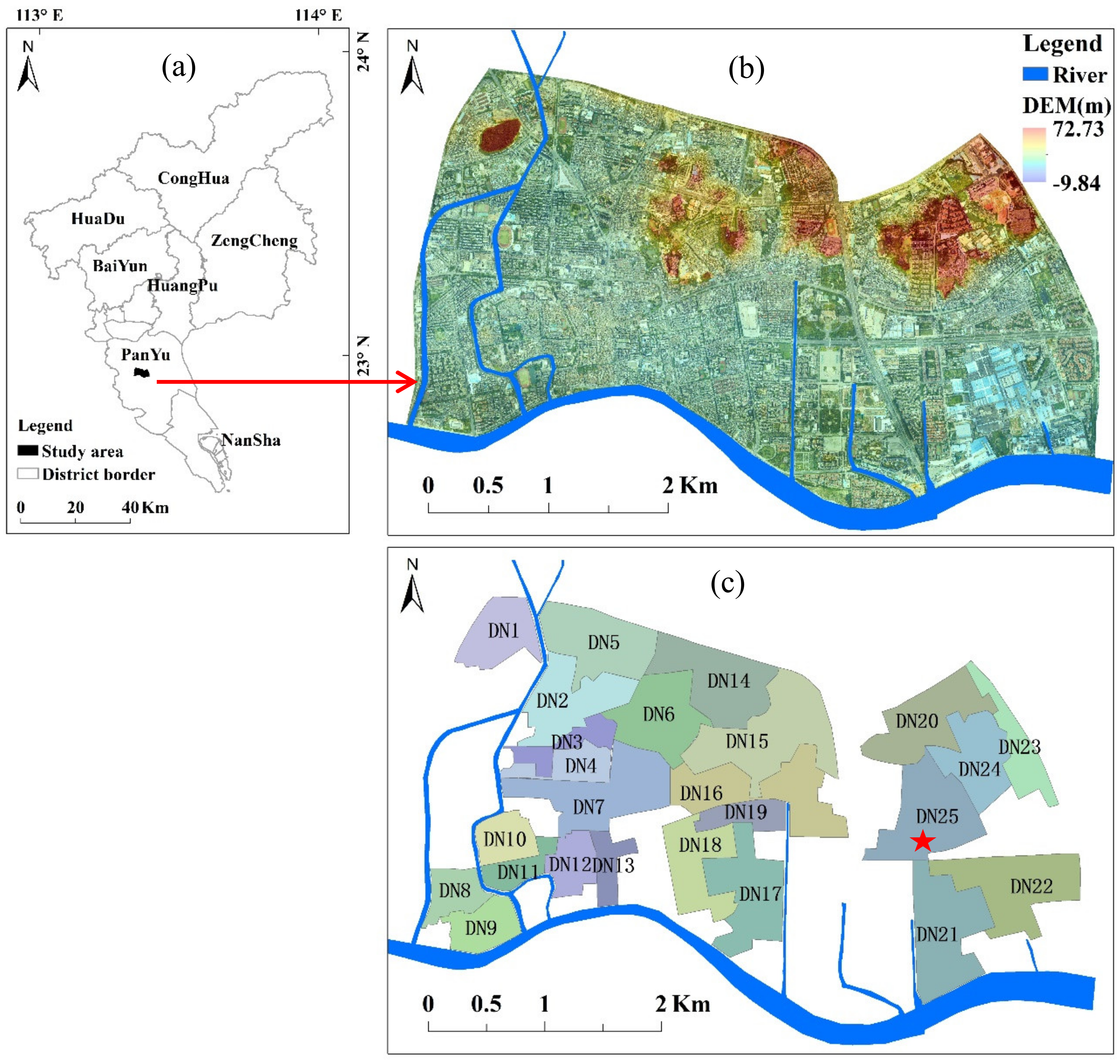
The study area is downtown of Panyu District, Guangzhou, China (Figure 2), which has an annual rainfall of about 1800 mm. This area has experienced rapid urbanization in recent decades and is currently about 74.5% impermeable. The sewer system was designed to cope with the rainfall events of a 1 year return period. The surface topography is represented by a Digital Elevation Model (DEM) of 1 m resolution, which was produced by the Light Detection and Ranging (LiDAR) technology in 2014. Land cover is classified into pervious and impervious surfaces using a 0.1 m resolution aerial image [57], which was acquired at the same time with the LiDAR DEM. Soil data come from the Harmonized World Soil Database version 1.1. Detailed pipe data, including pipe length, pipe diameter, and invert elevation, are collected from the original AutoCAD format.

2.2. Pressure Flow Simulation

2.2.1. SWMM

A SWMM in the study area was established, calibrated, and validated by Pan et al. in 2017 [58]. A monitoring system including a rain gauge and electronic water-depth meter was installed at the location shown in Figure 2c, where flood inundation has occurred several times each year. The in-situ measured rainfall depth and the derived street flooding volume were used to calibrate and validate the model. The flooding volume was calculated using recorded flood depths and the 1 m LiDAR DEM. In this study, the validated model is applied to simulate flood processes under multiple rainfall scenarios. Further, 25 independent drainage networks were identified in the model by means of the spatial relationship of drainage pipes, as shown in Figure 2c. The areas that have few pipes or which directly drain into rivers are not included in the analysis because their pipe systems have a limited impact on the storm drainage compared to large networks or upstream areas.

2.2.2. Rainfall Scenarios

The hourly rainfall depths for typical return periods are listed in Table 1 according to the local “Intensity-Duration-Frequency” relationships released by the Guangzhou Bureau of Water Authority [59]. The unequal intervals of rainfall depth among typical return periods are not convenient for analyzing the changing pattern and thus, rainfall scenarios from 5 to 115 mm are designed with an equal interval of 5 mm to reflect the impact of rainfall depth more intuitively. The performance in a single return period can be represented by the closest scenario. For instance, the last design storm has a similar rainfall depth (115 mm) with the 100 year return period (114 mm).
The temporal distribution of rainfall process is represented using the Chicago curve [60]. The rising and falling limbs are represented in Equation (1):
q t b = a 1 n t b 1 r + b t b 1 r 1 + n q t a = a 1 n t a r + b t a r + b 1 + n a = 167 A 1 1 + F × l o g T ,
where q(tb) and q(ta) are the time series of rainfall intensity in the rising and falling limbs, respectively; tb and ta are the time before and after the peak rainfall intensity, respectively; r is the ratio of the peak rainfall intensity time to the total duration and is set as 0.33; A1 is the rainfall depth (mm) for the 1 year return period, F is the parameter of rainfall depth variations, T is return period (year), b is used to adjust rainfall duration, and n is related to rainfall attenuation. The values of F, b, and n are 0.438, 11.259, and 0.750, respectively [59].

2.2.3. Runoff Generation

The runoff is calculated using the Soil Conservation Service—Curve Number method (SCS-CN) [61], a widely applied procedure for computing runoff from single-event design storms. The SCS-CN runoff equations are:
R = P I a 2 P I a + S S = 25400 C N 254 ,
where R is the runoff depth (mm), P denotes the rainfall depth (mm) of the storm event, Ia is all losses (mm) before runoff begins, S means the potential maximum soil retention (mm), and CN is the runoff curve number. Ia is highly variable, but generally is correlated with soil and land cover parameters. The empirical relationship between Ia and S is applied as
I a = 0.2 S .
S is related to the soil and cover conditions through CN, which has a range from 0 to 100. Typical runoff curve numbers for various cover type, imperviousness, and hydrologic soil group are also given [62]. In order to reflect the difference in impervious surface, composite runoff curve number is computed as
C N c = C N p + P i m p 100 98 C N p ,
where CNc is the composite runoff curve number, CNp is the pervious runoff curve number, and Pimp is the percentage of imperviousness [62]. The CNp is set as 73 in this study.

2.2.4. Flood Volume

In the SWMM, the overflow from surcharged junctions is the source of surface flooding. The flood volume of a drainage network under a certain rainfall scenario is the sum of the overflow from all junctions of the drainage network. There are 575 simulations in total for the 25 drainage networks under rainfall scenarios from 5 to 115 mm.

2.3. Pressure Flow Representation

2.3.1. Drainage Ratio

We propose a Drainage Ratio (DR) to measure the effect of pressure flow against the free surface flow in Equation (5)
D R = D D r R R r ,
where R and Rr are the runoff generated under the given (P) and reference (Pr) rainfall scenarios and D and Dr are the amount of runoff drained out by sewer pipes under the given and reference rainfall scenarios, respectively. The runoff (R and Rr) is estimated by the SCS-CN method. The pipe drainage under pressure flow (D and Dr) is simulated by the SWMM. The DR of a drainage network ranges from 0 to 1, depending on the hydraulic characteristics of the network and the reference rainfall scenario Pr.
In the CPD model, we assume that no flooding occurs if the precipitation is less than Pr. In other words, all drainage networks could effectively drain out the runoff generated by Pr. Flooding occurs when the precipitation is more than Pr, and the flood volume is the residual runoff ( R R r ) generated by the actual precipitation P and the reference precipitation Pr, i.e., D = D r . As a result, the DR of each network equals zero.
In this study, the reference rainfall (Pr = 55 mm) corresponds to a 1 year return period. The rainfall scenarios used for the test range from 60 to 115 mm, with an increasing interval of 5 mm. The testing rainfall period is 1 h. When this method is applied to other sewer networks, the new reference rainfall scenario Pr must be determined according to the local rainfall and drainage criteria.

2.3.2. Correlation Analysis with Influential Factors

The Pearson correlation is used to measure the effect of influential factors on pressure flow drainage, using a drainage network as a sample. The value of all influential factors is calculated on the basis of a drainage network. Four single factors and two compound indices are employed. The single factors include catchment area, pipe length, pipe slope, and pipe cross section area. Catchment area and pipe length are the same as those set up in the SWMM. Pipe slope and cross section area are defined as the average weighted by pipe length in Equations (6):
S p i p e = i = 1 N S i L i i = 1 N L i C = i = 1 N C i L i i = 1 N L i ,
where Spipe and C are the averages of pipe slope and the cross section area of a drainage network, respectively. Si, Ci, and Li are slope, cross section area, and length for the ith pipe, respectively, and N is the number of pipes in the drainage network.
We propose a new compound index, Velocity Ratio (VR), defined in Equations (7)–(9):
VR = V p i p e V i d e a l
V p i p e = S p i p e 1 / 2
V i d e a l = A × R C × t ,
where Vpipe (dimensionless) is the runoff velocity and Videal (m/s) is the average flow velocity that is required for a drainage network to completely drain out runoff through the cross section area C (m2) of pipes over the storm duration t (s). A (m2) is the catchment area of the drainage network and R (m) is the runoff depth. Representing the runoff velocity by the square root of pipe slope is inspired by the Gauckler-Manning formula [63], in which flow velocity is linearly proportional to the square root of the hydraulic slope.
We substitute Equations (8) and (9) into (7) and finally obtain the VR in Equation (10):
VR = S p i p e 1 / 2 × C × t A × R .
When the pipe slope is unavailable, we compute another VRs by replacing the pipe slope with the mean land surface slope in Equation (11):
V R s = S s u r f 1 / 2 × C × t A × R .

2.3.3. Regression Model

The most influential factor (VR) identified in the correlation analysis is used to establish a linear model to estimate the DR from VR in Equation (12):
D R = k × V R + e ,
where k is the coefficient and e is the estimated error.
In order to establish the regression model, the drainage networks are divided into two groups. One group (13 networks) with odd numbers (DN1, DN3, DN5, …, DN23, and DN25) is used to derive k and e for model calibration and the other group (12 networks) with even numbers (DN2, DN4, DN6, …, DN22, and DN24) is used to validate the model. The performance of the regression model is assessed by Mean Absolute Deviation (MAD) and the Square of the correlation coefficient (R2) between two DRs estimated by the regression model and simulated by the SWMM under the rainfall scenarios from 60 to 115 mm.

2.4. Flood Volume Adjustment

The flood water (total volume) can be calculated by multiplying the DR estimated by the regression model and the runoff increase (RRr) when the given rainfall is heavier than the reference rainfall (55 mm in an hour) in Equation (13):
F V = R R r × 1 D R ,
where FV is the total volume of flood water in a drainage network.
In the CPD model, no flood occurs when the rainfall depth is less than the reference rainfall depth, e.g., 55 mm in this study, and all runoff generated by the increasing rainfall becomes flood water (RRr). However, when R > Rr, the pipe drainage is not the free surface flow any more, but pressure flow, which could increase the flow speed and drain out more water than Dr. Therefore, the flood volume is overestimated by the CPD model and needs to be adjusted based on the effect of pressure flow on pipe drainage. When the pipe data are not available, pressure flow cannot be simulated by the SWMM or other hydraulic models, but the regression model of Equations (12) and (13) is an effective alternative to represent pressure flow and reduce the flood volume uncertainty caused by the CPD model.
Determining the actual capability of drainage networks is crucial for applying adjustments based on the VR. In the adjustment, all drainage networks are assumed capable of draining out runoff generated by the reference rainfall event. As a result, the flood volume at the reference rainfall depth, e.g., 55 mm in this study, is zero for all drainage networks. However, the assumption may be invalid because the drainage capacity is changing due to urban development or inadequate maintenance. If so, the flood volume at the reference rainfall depth can be larger than zero and systematic underestimations will occur. Further adjustment to the initial flood volume is still needed and solved in the results section.

3. Results

3.1. The Effect of Pressure Flow

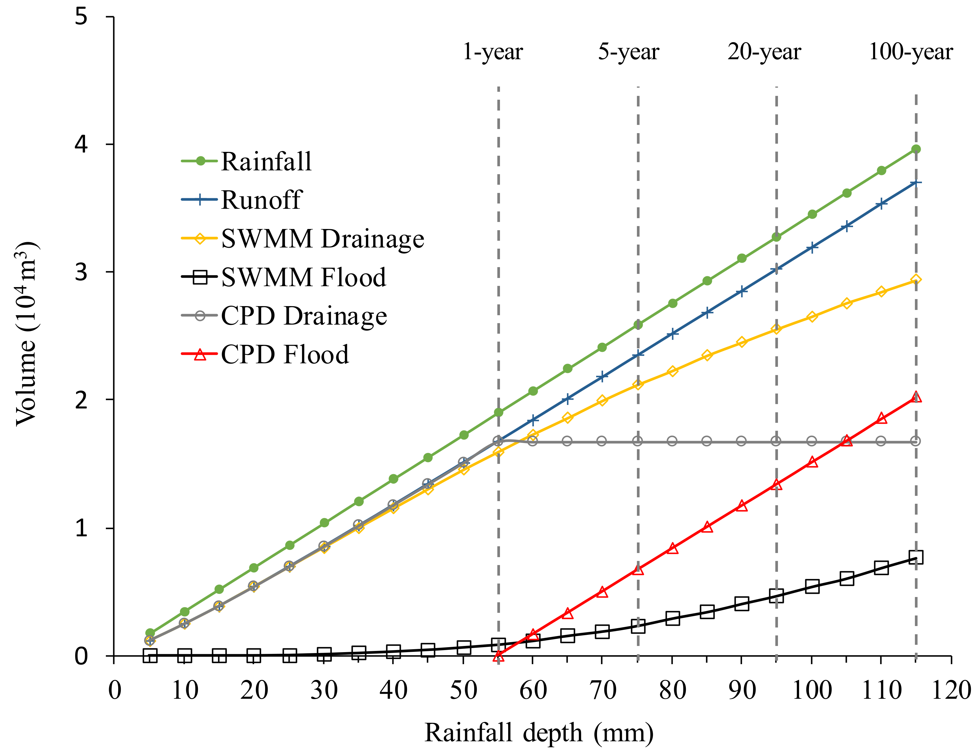
The CPD model neglects the effect of pressure flow and leads to significant bias in drainage and flood volumes, particularly for extreme rainfall events (Figure 3). The drainage volumes simulated by the SWMM increase monotonously with rainfall intensity at an attenuating rate. Accordingly, the simulated flood volumes increase at an escalating rate. In contrast, in the CPD model the drainage is assumed equal to the runoff until the reference rainfall depth (55 mm) and then remains stable under pressure flow. As a result, the gap in the flood volume between the SWMM and the CPD amplifies with rainfall intensity.
Besides the DN6 network illustrated in Figure 3, other drainage networks demonstrate a similar pattern that the flood volume increases with rainfall intensity. Due to the difference in the actual drainage capacity, the rainfall depth at which a network becomes flooded varies. Nevertheless, most networks get flooded at 55 mm, with the exceptions in DN4 and DN12, which get flooded at 75 mm and 80 mm, respectively. The DR of a drainage network decreases with increasing rainfall intensity, and the minimum and maximum DRs in the networks are listed in Table 2. It is clear that pressure flow helps drain out more storm water when the rainfall exceeds the reference value. What are the most influential factors controlling the pressure flow?

3.2. Significant Factors Affecting Pressure Flow

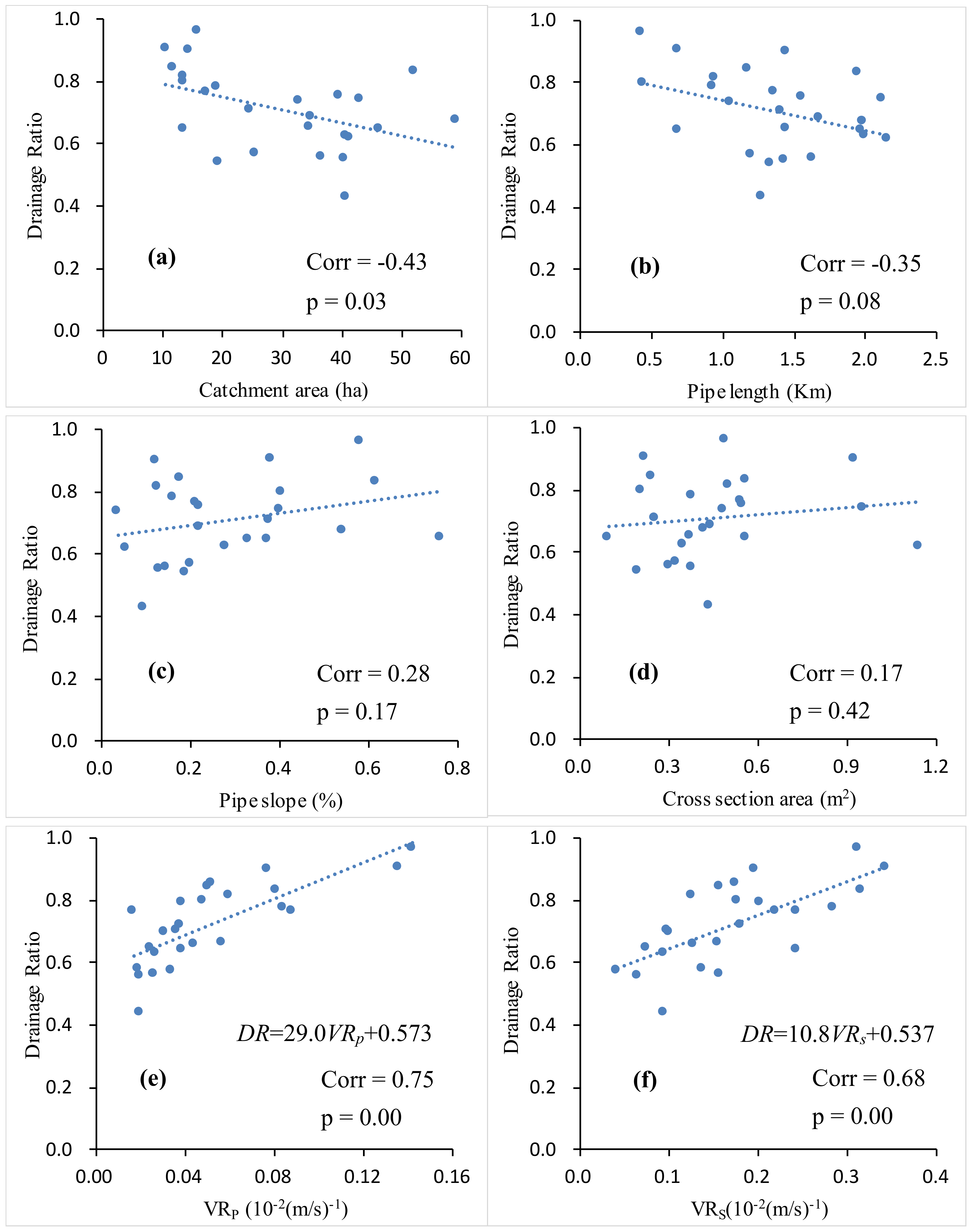
The two compound indices, VRp from pipe slope and VRs from surface slope, demonstrate the largest and significant correlation coefficients with DR among the six influential factors under the rainfall of a 100 year return period (Figure 4e,f). Catchment area and pipe length have a negative relationship with DR (Figure 4a,b) and pipe slope and cross section area have a positive effect on DR (Figure 4c,d). Table 3 summarizes the correlation coefficients between DR and the influential factors under six typical rainfall scenarios. They show similar results with Figure 4. Catchment area, VRp and VRs are significantly associated with DR under all rainfall scenarios at the confidence level 95%. Catchment area and pipe length are negatively correlated to DR, indicating that large areas or long distances are not beneficial for drainage. For a given rainfall event, a larger catchment area usually generates more runoff. Moreover, the pipe length is strongly related to the catchment area with a correlation coefficient of 0.81.
The VRp has the largest correlation coefficients among all influential factors. Compared to the four single factors, the VRp has a clear physical basis by integrating the catchment area, pipe slope, pipe cross section area, and runoff depth in Equation (10). The correlation coefficients range from 0.68 to 0.75, showing an increasing trend with rainfall intensity. One probable explanation is that the flow speed increases with higher pressure and the effect of pressure flow increases with rainfall intensity. When the pipe slope in VR is replaced by the surface slope, the correlation coefficients (0.64–0.68) are slightly smaller, but are still much higher than the single factors and significant at the confidence level of 95% (Table 3), suggesting that the VRs can be used as a valid variable to estimate the DR or the effect of pressure flow when the pipe data are not available.

3.3. Estimate of Drainage Ratio under Pressure Flow

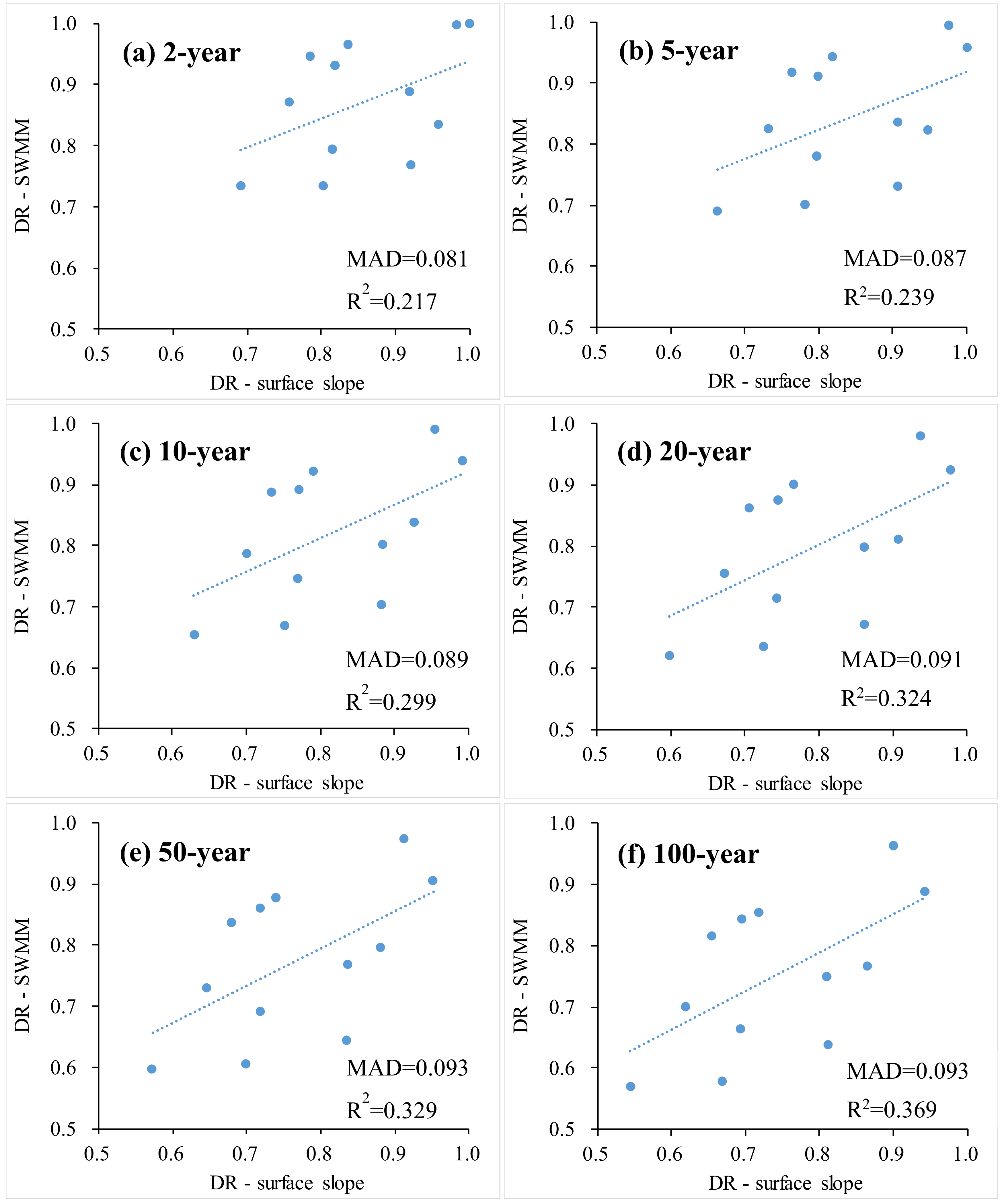
The regression models derived from 13 drainage networks in the calibration group for the six typical rainfall scenarios are summarized in Table 4. The DR of other 12 drainage networks in the validation group is estimated by these models using the VRs and is compared to the DR simulated by the SWMM (Figure 5). From the scatter plots, we can observe a clear positively correlated pattern between estimated and simulated DR. However, the samples do not cluster close to the fitted lines, reflected by the R2 at a relatively low level (0.217–0.369). The R2 increases with the rainfall intensity in both calibration and validation, indicating that the model tends to have a larger power representing the pressure flow under heavier rainfall events. The Mean Absolute Deviation (MAD) shows a slightly deteriorating trend with the rainfall intensity even if the R2 becomes better. A possible reason is that the range of DR value expands from a 2 year return period (0.73–1.0, Figure 5a) to a 100 year return period (0.57–0.96, Figure 5f). Nevertheless, the estimated DR agrees with the simulated DR at an acceptable level in terms of the MAD, which ranges from 0.081 to 0.093.

3.4. Flood Volume under Pressure Flow

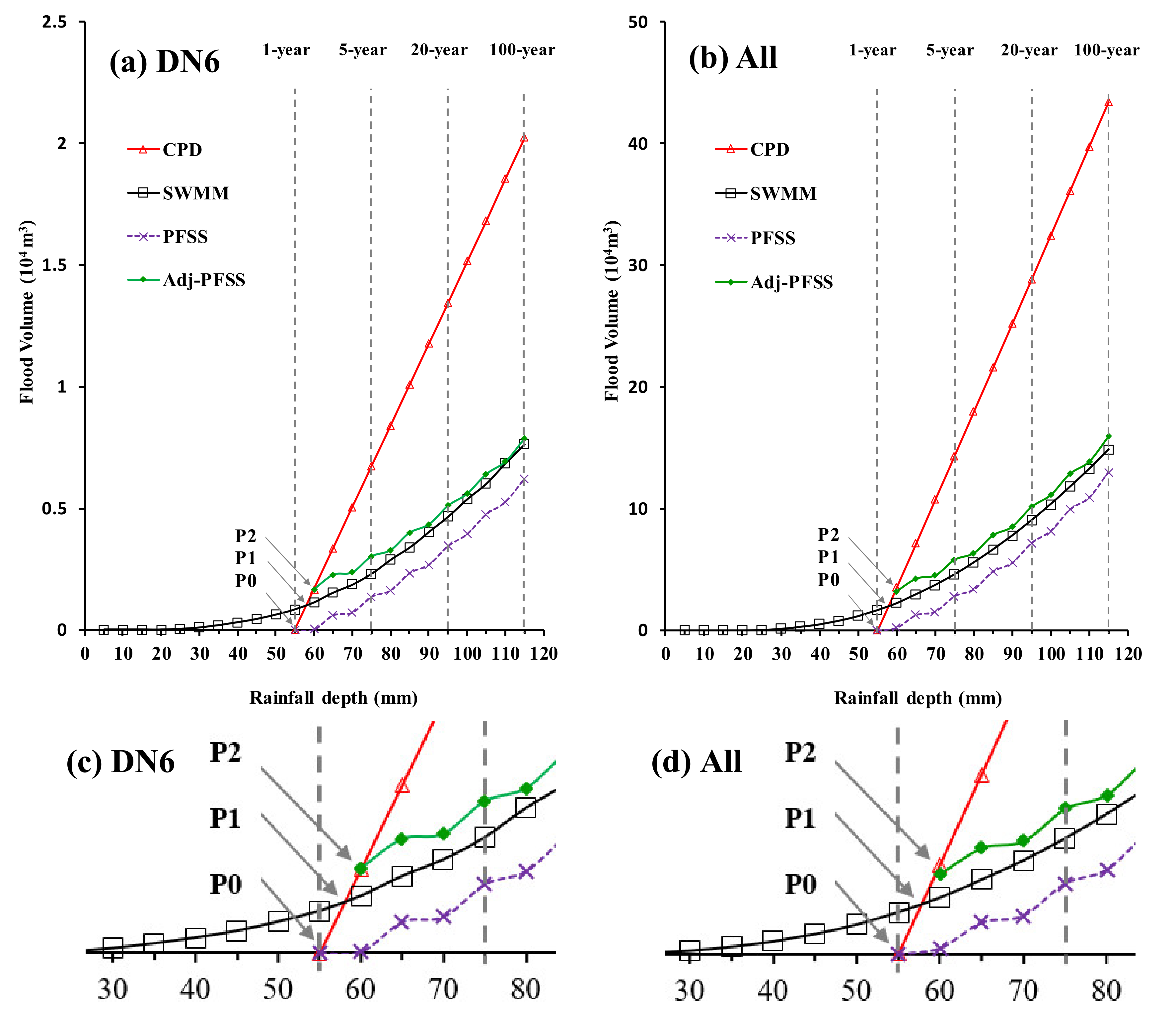
The flood volume can be calculated in Equation (13) using the runoff increase and the DRs estimated by the regression models in Table 4. The estimated flood volumes are compared with those simulated by the SWMM and the CPD (Figure 6). The curves of estimated flood volume using VRs, Pressure Flow using Surface Slope (PFSS), are under the SWMM curves for both network DN6 (Figure 6a) and all 25 networks as a whole (Figure 6b). The cause of underestimation is the non-zero flood volume at 55 mm on the SWMM curve. The PFSS curve intersects with the CPD curve at “P0”. Ideally, the adjustment should be made at “P1”, which is the intersection of CPD and SWMM curves. However, the accurate location of “P1” is unknown in practice. An alternative approach is to make the adjustment at a certain place like “P2” on the CPD curve, which is close to the reference rainfall scenario of 55 mm. If the intersection is moved to “P2” at 60 mm, the adjusted PFSS curves fit the SWMM curves much better than the PFSS at “P0”. The performances of three models, CPD, PFSS, and adjusted PFSS, are measured by the MAD and Mean Relative Deviation (MRD), as listed in Table 5. Clearly, regression models using surface slope can significantly reduce the uncertainty in flood volume estimated by the CPD. Moreover, the adjusted PFSS curve is slightly above the SWMM curve, conforming to the conservative principle in the flood risk analysis.

4. Discussions

4.1. Representation of Pressure Flow

The new index VR presented in this study provides a simplified representation of pressure flow, which frequently occurs in urban sewer systems, particularly under extreme rainfall events. The pipe flow transits from free-surface flow to pressure flow when the pipes become surcharged. Pressure flow is affected by multiple factors such as rainfall intensity, land cover, the spatial layout of sewer systems, local inundation depth, and boundary conditions. The accurate representation of pressure flow relies on hydrodynamic models with high-resolution data including surface land cover and subsurface sewer pipes. However, the lack of pipe data hinders the application of hydrodynamic models that implement the dual-drainage concept. This study proves that VR using surface slopes is strongly associated with pressure flow and can be applied to derive reasonable flood volumes when detailed pipe data are unavailable.
Although the VR-based model represents pressure flow satisfactorily in this study, it still has limitations. Firstly, with respect to flood volume, the 18% relative deviation cannot be neglected despite the fact that the VR-based model significantly outperforms the CPD model. Secondly, the VR-based model is not able to describe the flood status at single hydraulic features such as junction and conduit because it is designed to work on the basis of a drainage network. Furthermore, unlike hydrodynamic models that can directly output detailed flooding information including volume, velocity, time, and location, the VR-based model only provides flood volume. The inundating depth could be derived from flood volume with the aid of fine DEM data.

4.2. Applications

A direct application of our research is to evaluate the consistency of drainage designs using the VR from pipe slope in the planning phase. For an independent drainage network, the capacities of upstream branches should match that of the downstream areas. Otherwise, the sewer system cannot work properly. Consistency can be assessed by the difference in the VR between upstream branches and the whole drainage network. The regions with lower VR are the bottle neck of the drainage network and thus should be the target of further adjustment. Evaluation using the VR can significantly improve the efficiency of drainage design assessment compared with costly hydrodynamic simulations.
Another application is to assess the flood severity and to estimate the optimal pipe size and cost required for drainage projects. For a specific area, a larger pipe size required to instantly drain out storm water usually demands a higher cost, otherwise severe flooding would occur. The optimal pipe size can be estimated using Equation (9) by balancing the cost and tolerance to flood severity. Given a rainfall scenario (R), catchment area (A) and duration (t), the optimal pipe size (C) can be determined if the velocity term (Videal) is known. The Videal can be set as the maximum safe flow velocity according to the local drainage design code.

5. Summary and Remark

This research presents a simplified representation of pressure flow using a Velocity Ratio (VR)-based model, aiming to reduce the uncertainty of flood volume estimated by the CPD model when detailed pipe data are unavailable. The case study in Guangzhou, China was used to evaluate the performances of the VR-based model and the CPD model under typical rainfall events from 1 year to 100 year return periods. The simulated results from the well-known SWMM were applied as the reference.
The CPD model neglects the effect of pressure flow and leads to significant overestimation of flood volume. The overestimation is amplified with increasing rainfall intensity. In contrast, the VR-based model using surface slope can derive a reasonable amount of flood water. The estimated flood volumes for all networks agree with those simulated by the SWMM and have much smaller deviations (MAD 0.97 × 10⁴ m3 and MRD 18%) than those simulated by the CPD (MAD 15.69 × 10⁴ m3 and MRD 192%). Therefore, the VR-based model is an effective alternative to hydraulic models, especially in areas lacking detailed pipe data.
The VR is a simplified representation of pressure flow and is designed to estimate flood volumes on the basis of drainage networks. It cannot describe the status of singe hydraulic features such as junction and conduit, nor provide hydraulic information like the surface flow velocity, although the inundating depth could be estimated from flood volume with the aid of fine DEM data.
The general capability of the VR-based model needs further tests under distinct urban settings such as multiple land use/land cover, climate, and terrain conditions, and combined or separate sewer systems. Furthermore, it is worth exploring the potential of the VR-based model in calibrating and validating hydraulic models.

Author Contributions

Conceptualization, H.H. and X.W.; methodology, H.H. and X.W.; software, Y.P.: validation, H.H.; formal analysis, H.H. and X.W.; investigation, X.W.; resources, H.H.; data curation, Y.P.; writing—original draft preparation, H.H.; writing—review and editing, H.H. and X.W.; visualization, Y.P.; supervision, X.W.; project administration, H.H. and X.W.; funding acquisition, H.H. and X.W. All authors have read and agreed to the published version of the manuscript.

Funding

This research was funded by the National Key Research and Development Program of China (#2018YFB0505500, #2018YFB0505502), the National Natural Science Foundation of China (#41871085), the Water Resource Science and Technology Innovation Program of Guangdong Province (#2016-19), and the Science and Technology Program of Guangzhou (#201707010098).

Acknowledgments

We appreciate the language editing by Mark Jayne at School of Geography and Planning, Sun Yat-sen University.

Conflicts of Interest

The authors declare no conflict of interest. The funders had no role in the design of the study; in the collection, analyses, or interpretation of data; in the writing of the manuscript, or in the decision to publish the results.

References

  1. University of Maryland, Center for Disaster Resilience, and Texas A&M University, Galveston Campus, Center for Texas Beaches and Shores. The Growing Threat of Urban Flooding: A National Challenge; A. James Clark School of Engineering: College Park, MD, USA, 2018. [Google Scholar]
  2. Abhas, K.J.; Robin, B.; Jessica, L. Cities and Flooding: A Guide to Integrated Urban Flood Risk Management for the 21st Century; World Bank Group: Washington, DC, USA, 2012. [Google Scholar]
  3. Rubinato, M.; Nichols, A.; Peng, Y.; Zhang, J.; Lashford, C.; Cai, Y.; Lin, P.; Tait, S. Urban and river flooding: Comparison of flood risk management approaches in the UK and China and an assessment of future knowledge needs. Water Sci. Eng. 2019, 12, 274–283. [Google Scholar] [CrossRef]
  4. Apel, H.; Aronica, G.T.; Kreibich, H.; Thieken, A.H. Flood risk analyses—How detailed do we need to be? Nat. Hazards 2009, 49, 79–98. [Google Scholar] [CrossRef]
  5. Park, K.; Lee, M.H. The development and application of the urban flood risk assessment model for reflecting upon urban planning elements. Water 2019, 11, 920. [Google Scholar] [CrossRef] [Green Version]
  6. Eini, M.; Kaboli, H.S.; Rashidian, M.; Hedayat, H. Hazard and vulnerability in urban flood risk mapping: Machine learning techniques and considering the role of urban districts. Int. J. Disaster Risk Reduct. 2020, 50, 101687. [Google Scholar] [CrossRef]
  7. Egger, C.A.B.; Maurer, M.A.B. Importance of anthropogenic climate impact, sampling error and urban development in sewer system design. Water Res. 2015, 73, 78–97. [Google Scholar] [CrossRef]
  8. Huang, H.; Chen, X.; Zhu, Z.; Xie, Y.; Liu, L.; Wang, X.; Wang, X.; Liu, K. The changing pattern of urban flooding in Guangzhou, China. Sci. Total Environ. 2018, 622, 394–401. [Google Scholar] [CrossRef]
  9. Huang, H.; Zhang, L.; Liu, L.; Wang, X.; Wang, X.; Pan, C.; Wang, D. Assessing the mitigation effect of deep tunnels on urban flooding: A case study in Guangzhou, China. Urban Water J. 2019, 16, 312–321. [Google Scholar] [CrossRef]
  10. Xia, J.; Zhang, Y.Y.; Xiong, L.H.; He, S.; Wang, L.F.; Yu, Z.B. Opportunities and challenges of the Sponge City construction related to urban water issues in China. Sci. China Earth Sci. 2017, 60, 652–658. [Google Scholar] [CrossRef]
  11. Li, H.; Ding, L.; Ren, M.; Li, C.; Wang, H. Sponge city construction in China: A survey of the challenges and opportunities. Water 2017, 9, 594. [Google Scholar] [CrossRef] [Green Version]
  12. Jiang, Y.; Zevenbergen, C.; Ma, Y. Urban pluvial flooding and stormwater management: A contemporary review of China’s challenges and “sponge cities” strategy. Environ. Sci. Policy 2018, 80, 132–143. [Google Scholar] [CrossRef]
  13. Lashford, C.; Rubinato, M.; Cai, Y.; Hou, J.; Abolfathi, S.; Coupe, S.; Charlesworth, S.; Tait, S. SuDS & sponge cities: A comparative analysis of the implementation of pluvial flood management in the UK and China. Sustainability 2019, 11, 213. [Google Scholar]
  14. Mignot, E.; Li, X.; Dewals, B. Experimental modelling of urban flooding: A review. J. Hydrol. 2019, 568, 334–342. [Google Scholar] [CrossRef] [Green Version]
  15. Bulti, D.T.; Abebe, B.G. A review of flood modeling methods for urban pluvial flood application. Model. Earth Syst. Environ. 2020, 6, 1293–1302. [Google Scholar] [CrossRef]
  16. Djordjević, S.; Prodanović, D.; Maksimović, Č. An approach to simulation of dual drainage. Water Sci. Technol. 1999, 39, 95–103. [Google Scholar] [CrossRef]
  17. Schmitt, T.G.; Thomas, M.; Ettrich, N. Analysis and modeling of flooding in urban drainage systems. J. Hydrol. 2004, 299, 300–311. [Google Scholar] [CrossRef]
  18. Djordjević, S.; Prodanović, D.; Maksimović, Č.; Ivetić, M.; Savić, D. SIPSON—Simulation of interaction between pipe flow and surface overland flow in networks. Water Sci. Technol. 2005, 52, 275–283. [Google Scholar] [CrossRef]
  19. Rubinato, M.; Martins, R.; Kesserwani, G.; Leandro, J.; Djordjevic, S.; Shucksmith, J. Experimental investigation of the influence of manhole grates on drainage flows in urban flooding conditions. In Proceedings of the 14th IWA/IAHR International Conference on Urban Drainage, Prague, Czech Republic, 10–15 September 2017. [Google Scholar]
  20. Rubinato, M.; Lee, S.; Martins, R.; Shucksmith, J.D. Surface to sewer flow exchange through circular inlets during urban flood conditions. J. Hydroinform. 2018, 20, 564–576. [Google Scholar] [CrossRef] [Green Version]
  21. Beg, M.N.A.; Carvalho, R.F.; Tait, S.; Brevis, W.; Rubinato, M.; Schellart, A.; Leandro, J. A comparative study of manhole hydraulics using stereoscopic PIV and different RANS models. Water Sci. Technol. 2018, 2017, 87–98. [Google Scholar] [CrossRef]
  22. Rubinato, M.; Martins, R.; Shucksmith, J.D. Quantification of energy losses at a surcharging manhole. Urban Water J. 2018, 15, 234–241. [Google Scholar] [CrossRef] [Green Version]
  23. Del Giudice, G.; Gisonni, C.; Hager, W.H. Supercritical flow in bend manhole. J. Irrig. Drain. Eng. 2000, 126, 48–56. [Google Scholar] [CrossRef]
  24. Del Giudice, G.; Hager, W.H. Supercritical flow in 45° junction manhole. J. Irrig. Drain. Eng. 2001, 127, 100–109. [Google Scholar] [CrossRef] [Green Version]
  25. Arao, S.; Kusuda, T.; Moriyama, K.; Hiratsuka, S.; Asada, J.; Hirose, N. Energy losses at three-way circular drop manholes under surcharged conditions. Water Sci. Technol. 2012, 66, 45–52. [Google Scholar] [CrossRef] [PubMed]
  26. Rubinato, M.; Shucksmith, J.; Saul, A.J.; Shepherd, W. Comparison between InfoWorks hydraulic results and a physical model of an Urban drainage system. Water Sci. Technol. 2013, 68, 372–379. [Google Scholar] [CrossRef] [PubMed]
  27. Bazin, P.H.; Nakagawa, H.; Kawaike, K.; Paquier, A.; Mignot, E. Modeling flow exchanges between a street and an underground drainage pipe during urban floods. J. Hydraul. Eng. 2014, 140, 4014051. [Google Scholar] [CrossRef]
  28. Rubinato, M. Physical scale modelling of urban flood systems. Ph.D. Thesis, University of Sheffield, Sheffield, UK, 2015. Available online: http://etheses.whiterose.ac.uk/9270/ (accessed on 25 June 2015).
  29. Rubinato, M.; Martins, R.; Kesserwani, G.; Leandro, J.; Djordjević, S.; Shucksmith, J. Experimental calibration and validation of sewer/surface flow exchange equations in steady and unsteady flow conditions. J. Hydrol. 2017, 552, 421–432. [Google Scholar] [CrossRef]
  30. Martins, R.; Rubinato, M.; Kesserwani, G.; Leandro, J.; Djordjević, S.; Shucksmith, J.D. On the Characteristics of Velocities Fields in the Vicinity of Manhole Inlet Grates During Flood Events. Water Resour. Res. 2018, 54, 6408–6422. [Google Scholar] [CrossRef]
  31. Leandro, J.; Chen, A.S.; Djordjević, S.; Savić, D.A. Comparison of 1D/1D and 1D/2D coupled (sewer/surface) hydraulic models for urban flood simulation. J. Hydraul. Eng. 2009, 135, 495–504. [Google Scholar] [CrossRef]
  32. Davidsen, S.; Löwe, R.; Thrysøe, C.; Arnbjerg-Nielsen, K. Simplification of one-dimensional hydraulic networks by automated processes evaluated on 1D/2D deterministic flood models. J. Hydroinform. 2017, 19, 686–700. [Google Scholar] [CrossRef] [Green Version]
  33. Yu, D.; Yin, J.; Liu, M. Validating city-scale surface water flood modelling using crowd-sourced data. Environ. Res. Lett. 2016, 11, 124011. [Google Scholar] [CrossRef]
  34. Jamali, B.; Bach, P.M.; Cunningham, L.; Deletic, A. A Cellular Automata Fast Flood Evaluation (CA-ffé) Model. Water Resour. Res. 2019, 55, 4936–4953. [Google Scholar] [CrossRef] [Green Version]
  35. Savant, G.; Trahan, C.J.; Pettey, L.; McAlpin, T.O.; Bell, G.L.; McKnight, C.J. Urban and overland flow modeling with dynamic adaptive mesh and implicit diffusive wave equation solver. J. Hydrol. 2019, 573, 13–30. [Google Scholar] [CrossRef]
  36. Su, B.; Huang, H.; Zhu, W. An urban pluvial flood simulation model based on diffusive wave approximation of shallow water equations. Hydrol. Res. 2019, 50, 138–154. [Google Scholar] [CrossRef]
  37. Yu, D.; Lane, S.N. Urban fluvial flood modelling using a two-dimensional diffusion-wave treatment, part 1: Mesh resolution effects. Hydrol. Process. 2006, 20, 1541–1565. [Google Scholar] [CrossRef]
  38. Yu, D.; Lane, S.N. Urban fluvial flood modelling using a two-dimensional diffusion-wave treatment, part 2: Development of a sub-grid-scale treatment. Hydrol. Process. 2006, 20, 1567–1583. [Google Scholar] [CrossRef]
  39. Singh, V.P.; de Lima, J.L.M.P. One-dimensional linear kinematic wave solution for overland flow under moving storms using the method of characteristics. J. Hydrol. Eng. 2018, 23, 04018029. [Google Scholar] [CrossRef]
  40. Cimorelli, L.; Morlando, F.; Cozzolino, L.; Covelli, C.; Della Morte, R.; Pianese, D. Optimal positioning and sizing of detention tanks within urban drainage networks. J. Irrig. Drain. Eng. 2016, 142, 04015028. [Google Scholar] [CrossRef]
  41. Bates, P.D.; De Roo, A.P.J. A simple raster-based model for flood inundation simulation. J. Hydrol. 2000, 236, 54–77. [Google Scholar] [CrossRef]
  42. Martins, R.; Leandro, J.; Djordjević, S. A well balanced Roe scheme for the local inertial equations with an unstructured mesh. Adv. Water Resour. 2015, 83, 351–363. [Google Scholar] [CrossRef]
  43. Bates, P.D.; Horritt, M.S.; Fewtrell, T.J. A simple inertial formulation of the shallow water equations for efficient two-dimensional flood inundation modelling. J. Hydrol. 2010, 387, 33–45. [Google Scholar] [CrossRef]
  44. Ghimire, B.; Chen, A.S.; Guidolin, M.; Keedwell, E.C.; Djordjević, S.; Savić, D.A. Formulation of a fast 2D urban pluvial flood model using a cellular automata approach. J. Hydroinform. 2013, 15, 676–686. [Google Scholar] [CrossRef] [Green Version]
  45. Issermann, M.; Chang, F.J.; Jia, H. Efficient urban inundation model for live flood forecasting with cellular automata and motion cost fields. Water 2020, 12, 1997. [Google Scholar] [CrossRef]
  46. Shao, Q.; Weatherley, D.; Huang, L.; Baumgartl, T. RunCA: A cellular automata model for simulating surface runoff at different scales. J. Hydrol. 2015, 529, 816–829. [Google Scholar] [CrossRef]
  47. Liu, L.; Liu, Y.; Wang, X.; Yu, D.; Liu, K.; Huang, H.; Hu, G. Developing an effective 2-D urban flood inundation model for city emergency management based on cellular automata. Nat. Hazards Earth Syst. Sci. 2015, 15, 381–391. [Google Scholar] [CrossRef] [Green Version]
  48. Chen, J.; Hill, A.A.; Urbano, L.D. A GIS-based model for urban flood inundation. J. Hydrol. 2009, 373, 184–192. [Google Scholar] [CrossRef]
  49. Gouldby, B.; Sayers, P.; Mulet-Marti, J.; Hassan, M.A.A.M.; Benwell, D. A methodology for regional-scale flood risk assessment. Proc. Inst. Civ. Eng. Water Manag. 2008, 161, 169–182. [Google Scholar] [CrossRef]
  50. Zhang, S.; Pan, B. An urban storm-inundation simulation method based on GIS. J. Hydrol. 2014, 517, 260–268. [Google Scholar] [CrossRef]
  51. Maksimović, Č.; Prodanovic, D.; Boonya-aroonnet, S.; Leitão, J.; Djordjević, S.; Allitt, R. Overland flow and pathway analysis for modelling of urban pluvial flooding. J. Hydraul. Res. 2010, 47, 512–523. [Google Scholar] [CrossRef]
  52. Lhomme, J.; Sayers, P.; Gouldby, B.; Samuels, P.; Wills, M. Recent development and application of a rapid flood spreading method. In Proceedings of the FLOODrisk, Keble College, Oxford, UK, 30 September–2 October 2008; pp. 15–24. [Google Scholar]
  53. Huang, H.; Chen, X.; Wang, X.; Wang, X.; Liu, L. A depression-based index to represent topographic control in urban pluvial flooding. Water 2019, 11, 2115. [Google Scholar] [CrossRef] [Green Version]
  54. Jamali, B.; Löwe, R.; Bach, P.M.; Urich, C.; Arnbjerg-Nielsen, K.; Deletic, A. A rapid urban flood inundation and damage assessment model. J. Hydrol. 2018, 564, 1085–1098. [Google Scholar] [CrossRef]
  55. Li, Z.; Wu, L.; Zhu, W.; Hou, M.; Yang, Y.; Zheng, J. A new method for urban storm flood inundation simulation with fine CD-TIN surface. Water 2014, 6, 1151–1171. [Google Scholar] [CrossRef]
  56. Zhao, G.; Xu, Z.; Pang, B.; Tu, T.; Xu, L.; Du, L. An enhanced inundation method for urban flood hazard mapping at the large catchment scale. J. Hydrol. 2019, 571, 873–882. [Google Scholar] [CrossRef]
  57. Cao, J.; Leng, W.; Liu, K.; Liu, L.; He, Z.; Zhu, Y. Object-Based Mangrove Species Classification Using Unmanned Aerial Vehicle Hyperspectral Images and Digital Surface Models. Remote Sens. 2018, 10, 89. [Google Scholar] [CrossRef] [Green Version]
  58. Pan, C.; Wang, X.; Liu, L.; Huang, H.; Wang, D. Improvement to the huff curve for design storms and urban flooding simulations in Guangzhou, China. Water 2017, 9, 411. [Google Scholar] [CrossRef] [Green Version]
  59. GBWA (Guangzhou Bureau of Water Authority). The Rainstorm Formula and Calculation Chart in Guangzhou Downtown. Guangzhou, China. 2011. Available online: http://www.cma.gov.cn/2011xwzx/2011xxdqxywtx/2011xzhgcxt/201110/t20111029_141510.html (accessed on 23 May 2011).
  60. Keifer, C.J.; Chu, H.H. Synthetic Storm Pattern for Drainage Design. J. Hydraul. Div. 1957, 83, 1–25. [Google Scholar]
  61. NRCS (Natural Resource Conservation Service). Urban Hydrology for Small Watersheds; Technical Release No. 55 (TR-55); USDA: Washington, DC, USA, 1986. [Google Scholar]
  62. NRCS (Natural Resource Conservation Service). National Engineering Handbook; Part 630; USDA: Washington, DC, USA, 2009. [Google Scholar]
  63. Manning, R. On the flow of water in open channels and pipes. Trans. Inst. Civ. Eng. Irel. 1891, 20, 161–207. [Google Scholar]
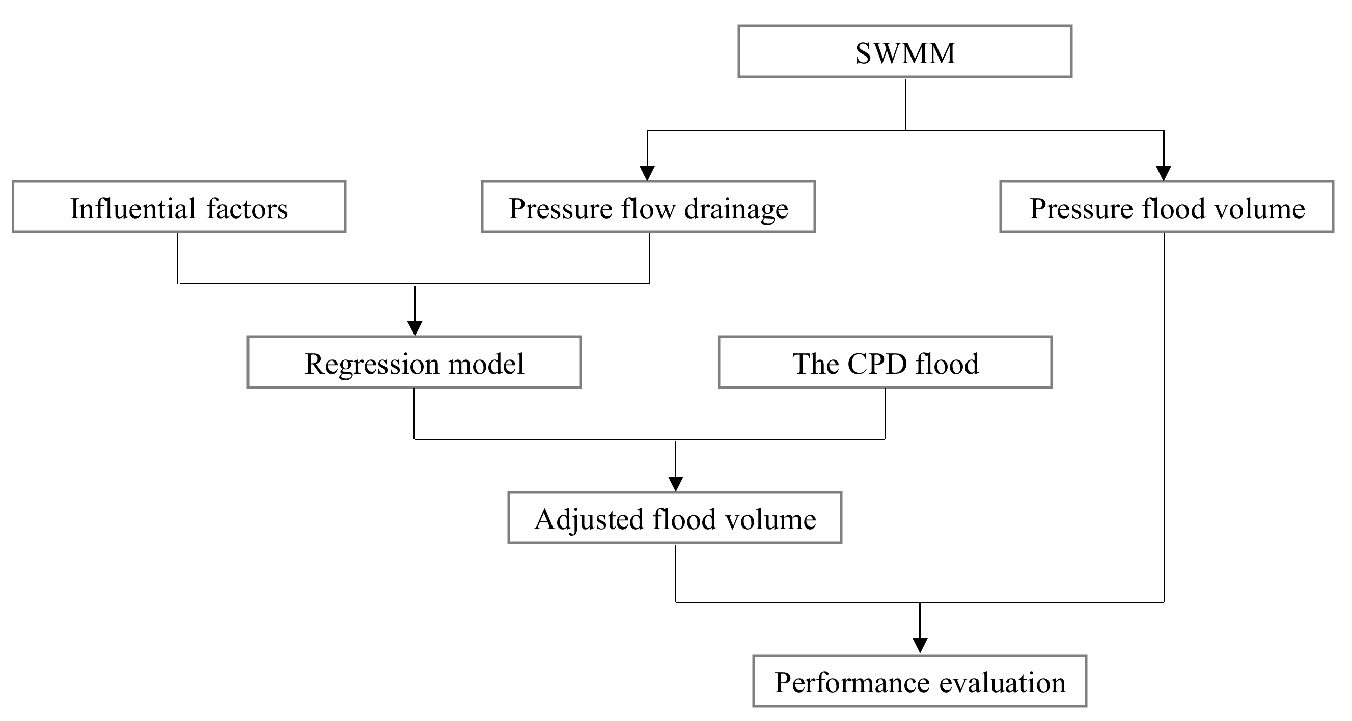
Figure 1. The flowchart to quantify the effect of pressure flow and adjust the flood volumes simulated by the Constant Pipe Drainage (CPD).
Water 12 02778 g001
Figure 2. The location of the study area in Guangzhou, China (a), its topography and aerial image (b), and 25 independent drainage networks (c). The location of the monitoring system is marked by a red pentagram in the drainage network DN25.
Water 12 02778 g002
Figure 3. Hydrological responses of the drainage network DN6 simulated by the SWMM and the CPD under the rainfall events from 5 to 115 mm. Four typical return periods are marked using vertical dashed lines. The key properties of DN6 are: (1) area, 34.4 ha; (2) imperviousness, 75.4%; (3) pipe length, 1.45 km; (4) average pipe slope, 0.76%; (5) average pipe cross section area, 0.371 m2; and (6) average surface slope, 5.88%.
Water 12 02778 g003
Figure 4. The scatter plots between the DR and six influential factors in the 25 drainage networks under the rainfall of a 100 year return period: catchment area (a), pipe length (b), pipe slope (c), pipe cross section area (d), Velocity Ratio (VR)p from pipe (e), and VRs from land surface slope (f). The pipe slope and cross section area are calculated using Equation (6). “Corr” is the Pearson correlation coefficient and “p” denotes the p-value in the statistical significance test.
Water 12 02778 g004
Figure 5. The scatter plots between the DR estimated by the regression models using VRs and by the SWMM in the 12 networks for the six typical rainfall scenarios.
Water 12 02778 g005
Figure 6. Comparison of flood volumes derived by pressure flow (SWMM), free surface flow (CPD), and the regression model using surface slope (PFSS) for the drainage network DN6 (a) and all 25 networks (b). “PFSS” stands for Pressure Flow using Surface Slope and “Adj-PFSS” means the empirical adjustment using the flood volume at the rainfall depth of 60 mm. Four typical return periods are marked by vertical dashed lines. Two zoom-in graphs, (c,d) are given to show the locations of P0, P1, and P2 in (a,b), respectively.
Water 12 02778 g006
Table 1. Average intensity and rainfall depth for design storms with typical return periods over a 1 h duration in Guangzhou, China.
Return Period
(Year)
Average Intensity
(L/(ha.s))
Rainfall Depth
(mm)
1151.355
2176.163
5209.776
10236.285
20263.695
50295.1106
100315.5114
Table 2. Drainage Ratios in all 25 drainage networks. “Min” and “Max” are the minimum and maximum Drainage Ratios (DRs), corresponding to the rainfall scenarios of 115 and 60 mm, respectively.
NetworkMinMaxNetworkMinMax
DN10.720.93DN140.770.84
DN20.700.88DN150.700.85
DN30.840.93DN160.840.94
DN40.891.00DN170.550.67
DN50.630.79DN180.570.74
DN60.660.82DN190.760.88
DN70.670.88DN200.580.76
DN80.850.97DN210.440.60
DN90.800.94DN220.640.79
DN100.820.97DN230.560.75
DN110.650.78DN240.750.93
DN120.961.00DN250.790.88
DN130.900.99
Table 3. Pearson correlation coefficients between the DR and influential factors under six typical return periods. The correlation analysis is based on all 25 networks, using one network as a sample. “*” and “#” denote the confidence levels of 95% (p-value 0.05) and 90% (p-value 0.1), respectively. “VRp” and “VRs” are the Velocity Ratio using pipe slope and surface slope, respectively.
Return PeriodCatchment AreaPipe LengthPipe SlopePipe Cross Section AreaVRpVRs
(Year)(ha)(km)(%)(m2)((m/s)−1)
2−0.48 *−0.37 #0.230.080.68 *0.64 *
5−0.47 *−0.36 #0.280.110.72 *0.65 *
10−0.44 *−0.33 #0.290.150.75 *0.68 *
20−0.43 *−0.34 #0.290.150.74 *0.68 *
50−0.43 *−0.35 #0.290.150.75 *0.68 *
100−0.43 *−0.35 #0.280.170.75 *0.68 *
Average−0.45 *−0.35 #0.280.130.73 *0.67 *
Table 4. The regression models between DR and VRs derived from 13 drainage networks in the calibration group for the six typical rainfall scenarios. The model performances in calibration and validation are also listed.
Return PeriodRegression EquationCalibrationValidation
R2R2MAD
2 yearDR = 1.795VRs + 0.6550.4980.2170.081
5 yearDR = 3.837VRs + 0.6140.5060.2390.087
10 yearDR = 6.008VRs + 0.5780.5190.2990.089
20 yearDR = 8.382VRs + 0.5440.5190.3240.091
50 yearDR = 10.506VRs + 0.5130.5130.3290.093
100 yearDR = 13.253VRs + 0.4880.5270.3690.093
Table 5. Performances of three models against the SWMM, measured by Mean Absolute Deviation (MAD) (104 m3) and Mean Relative Deviation (MRD).
DN6All Networks
MADMRDMADMRD
CPD0.70166%15.69192%
PFSS0.1240%2.0136%
Adj-PFSS0.0418%0.9718%