Abstract
Every network of supply waterlines experiences thousands of yearly bursts, breaks, leakages, and other failures. These failures waste a great amount of resources, as not only the waterlines need to be repaired, but also water is wasted and the distribution service is interrupted. For that reason, many water facilities employ proactive maintenance strategies in their networks, where they replace likely-to-fail pipes in advance to prevent the failures. In this paper, we aim to establish a reliable prediction model that can accurately predict faults in waterlines prior to their occurrence. We propose a specific segmentation method for long transmission mains, as well as three data-driven models and one rule-based prediction model. We evaluate a real world waterline network used in Israel, operated by Mekorot company, using three common metrics. The results show that the data-driven algorithms outperform the rule-based model by at least 5% in each of the metrics. Additionally, their prediction becomes more accurate as they are trained with more data, but enhancing these data with geographically related features does not improve the accuracy further.
1. Introduction
A continuous supply with drinking water strongly depends on the reliability of water transmission mains. Accurate models for predicting the deterioration state of the pipes are essential for scheduling maintenance or plan renewal of these vulnerable pipes. According to Scheidegger et al. [1] deterioration models for water mains can be differentiated by at least three dimensions: the smallest described entity (e.g., a single pipe, a pipe section or a partial network), the type of events that are modeled (a fault or the end of a pipes lifespan), and the modeled process (physical or statistical models). The three dimensions can be combined in any way [1].
Physical models try to describe the physical process of deterioration that leads to a fault and statistical models describe the occurrence of a fault as a stochastic process. Fault in this context is either a leak or a burst. While statistical models can be applied even in data scarcity situations, physical models demand a high degree of information on external as well as on intrinsic stress factors that influence the deterioration process. This makes the inspection of the pipes deterioration state necessary. Pipe inspection with either non-destructive or destructive techniques can be costly and the techniques are only applicable under specific boundary conditions. E.g., electromagnetic methods or stress waves-based methods either require the structure temporarily out of service to inspect from the inside or require excavation in order to conduct the inspection from the outside [2]. However, for highly vulnerable transmission mains, the application of inspection techniques might be economically viable. Nevertheless, prior to inspection, the application of failure models is of help, in order to prioritize pipes for inspection based on the likelihood of a bad deterioration state that is derived from the failure model.
Liu et al. [3] gave an overview on statistical and physical models as well as on the data needed for the application of the different models that can be found in literature. Scheidegger et al. [1] gave a comprehensive overview on statistical models, focusing on single pipe fault predictions. They concluded that from the reviewed models, no specific model structure exists that appears superior. For the selection of the most adequate pipe failure model, the following points should be taken into account: (i) the appropriate likelihood function should be selected based on the data characteristics; (ii) the model predictions should match the initial questions; and, (iii) the assumption of the failure model should be in agreement with the experience of the operator [1].
The scope of the this work is to develop an accurate method for predicting faults in water transmission mains. Kleiner and Rajani [4] mentioned that little work can be found on making decisions prior to water main failure, which is desirable for large water transmission mains, where failure consequences can be severe. Friedl et al. [5] described a method that allows for failure mode prediction as well as for vulnerability assessment to prioritise transmission mains for maintenance or inspection actions. The method was successfully used for fault prediction in two transmission mains systems, but it requires a large amount of historic data and detailed information on pipe characteristics and boundary conditions, which, in many cases, are not available in practice.
At water utilities, where GIS systems are used to store pipe and fault data, the generally available information on pipe characteristics is the pipe material, the diameter, and the age (respectively, the year of construction). These parameters are used as explanatory variables in most of the statistical models for water mains fault prediction. Kleiner and Rajani [6] described that pipe length has frequently been used as a covariate to ‘explain’ at least some of the variability observed in individual water mains (e.g. [7,8,9]). Additional failure history represented, as, e.g., the number of known previous failure, was found to be a significant parameter in pipe failure prediction [6].
In recent years, machine learning techniques have gathered some interest among researchers in the field of fault prediction in general and in the field of water in particular. For instance, Song et al. [10] present a method to predict vertical heterogeneity of the reservoir utilizing various deep neural networks based on dynamic production data. Zhang et al. [11] presented a method for predicting water saturation distribution in reservoirs with a machine learning method. In the context of pipe fault prediction, Wang et al. [12] used a RankBoostB and a neural network approach, as well as a Cox and Logistic Regression to predict faults in a water distribution system. They compared the performance of these four models based on the AUC (area under receiver operating curve). The comparisons have shown that RankBoostB outperforms the other algorithms, followed by the logistic regression model in the case study area, which was a distribution network in China. Giraldo-González and Rodríguez [13] tested Machine Learning approaches, particularly Gradient-Boosted Tree (GBT), Bayes, Support Vector Machines, and Artificial Neuronal Networks (ANNs), for predicting individual pipe failure rates and compared the models performance with data from a partial distribution network in Bogotá (Colombia). The results have shown that Bayes and ANNs exhibited low performance in the prediction of pipe failure and that the GBT approach had the best performing classifier. Berardi et al. [14] used evolutionary polynomial regression (EPR) for pipe deterioration modelling, as it yields symbolic formulae that are intuitive and easily understandable by practitioners. Snider and McBean [15] provide an in-depth comparison of the two leading statistical pipe-break modeling methods: machine-learning and survival-analysis algorithms. A gradient-boosting decision tree machine-learning model and a Weibull proportional hazard survival-analysis model are used to predict time to next break for cast-iron pipes in a major Canadian water distribution system. The authors concluded that water utilities concerned with short-term security arising from the impacts of pipe breaks on water security may favor the machine-learning approach, but the survival-analysis models’ ability to incorporate right-censored data makes it more appropriate for long-term asset management planning [15]. Alizadeh et al. [16] recently published work on data driven pipe burst prediction in urban water distribution systems. They used Grasshopper Optimization Algorithm-based Support Vector Regression (GOA-SVR), Gaussian Process Regression (GPR), and Artificial Neural Network (ANN) in order to predict the pipe burst rate in an urban area and showed that, in their case study, GPR could outperform the other algorithms.
Although data driven and machine learning based techniques for pipe fault prediction gathered a lot of interest among researchers in recent years, little work can be found on while using these techniques to predict faults in large transmission main systems so far. In this paper, a data driven approach for fault prediction on transmission mains is introduced, which allows for predicting the number of faults on a pipe segment in a defined future period of time (e.g., 1/2 year). Such a model is required for a better scheduling of maintenance actions prior to fault occurrence [4]. Scheidegger et al. [1] mention in their conclusions that faults on water pipes may have a spacial dependability and should be incorporated into failure prediction models. Further, Chen and Guikema [17] found that that use of spatial clusters, as an explanatory variable, can improve the accuracy of pipe break machine learning models. To take spacial dependability into account in fault prediction, a suitable segmentation of long transmission mains is needed.
The prediction method that is presented in this paper utilizes two algorithms (i) a pipe segmentation algorithm and (ii) a fault prediction algorithm. The pipe segmentation algorithm has the purpose of dividing the waterlines into meaningful segments, as waterlines are often very long, and thus indicating that a waterline will have a fault may not be specific enough to be useful in practice [18]. The fault prediction algorithm predicts the number of faults that will occur in a segment in the next period, where the length of the period is a parameter that can be determined by the user.
Evaluation was done on a real world transmission main system of Israel, which was operated by Mekorot company. Several metrics for evaluating the performance of the prediction models are presented. Among these metrics are Root Mean Squared Error (RMSE), Conover, and Kendal‘s Tau. The data driven algorithms provided better results than the expert rule-based model by at least 5%, 4%, and 13% in those three metrics, respectively. Further, we look at the impact of the training set size and of spacial dependabilities between faults.
The flow of the paper is as follows. Section 2 describes the segmentation methods of the waterlines as well as the fault prediction algorithms we utilized. Section 3 presents the results of the proposed algorithms. Section 4 discusses some of the limitations of our proposed methodology and Section 5 concludes.
2. Methodology
In this section, we describe the proposed prediction process, including a description of the segmentation methods (Section 2.1), the fault prediction methodology (Section 2.2), and the prediction algorithms (Section 2.3).
2.1. Segmentation Methods
A waterline length could be in a range of a few hundred meters to several kilometers. Predicting faults in such long waterlines is meaningless, since no water main company will replace waterlines this long [18,19]. To this end, the waterlines must be divided into segments. We divide the waterlines into segments in two different ways:
- Fixed. Dividing each waterline into segments of a fixed length. Specifically, we evaluated with fixed segmentation length of 360 m. This length was determined by the average length of the segments in the next dynamic segmentation method.
- Dynamic. The dynamic segmentation method was proposed by water main experts, being intended to provide a segmentation that is meaningful to water main companies use cases. We describe this segmentation method below.
The dynamic segmentation method is affected by the faults that were observed in the past and their distances along the waterlines. For each line, we group faults that occurred within 300 m of each other. Subsequently, each group that contains at least two faults defines a segment which starts 150 m before the first fault of the segment and ends 150 m after the last fault of the segment (The maximum size between faults, as well as the size of the margins are parameters that can be changed). Note that using this segmentation method dictates that all of the resulting segments shall have at least two faults.
In order to demonstrate this segmentation, assume a pipe that has had four faults, located 400, 500, 800, and 1500 m from the start of the pipe. Subsequently, the first three faults would be in a single group, since each one of them is located at most 300 m after the previous one. This group generates a segment that starts at 250 m and ends at 950 m from the start of the waterline. The fault at 1500 m is in another group by itself, since there are no other faults within 300 m and, therefore, it does not define a segment. Thus, we end up with a single 700 m long segment.
2.2. Fault Prediction Process
The second step is to run a learning algorithm that will output a prediction model that accepts a waterline segment and outputs a prediction of the number of faults this segment is expected to have in the next time period. In order to evaluate a prediction model, a third step is needed, in which the learned prediction model is evaluated [20].
Typically, learning algorithms generate a prediction model that is based on a dataset referred to as the training set, and evaluate the generated model on a different dataset, referred to as the test set. The training set, which is used to train the prediction model, includes segments that are associated with features and with a label. The features of a segment describe its characteristics, such as age, material, or length, while the label is the number of faults that occur in that segment. The learning algorithm aims to learn a function that maps between the features and the label. We call such a mapping a prediction model. Finally, the prediction model is evaluated while using the segments from the test dataset [21,22].
One main feature, recommended by experts from Mekorot, is the number of faults a segment had in the past—FaultCount. In order to utilize this feature, we split the dataset of past faults to three equal time periods: A, B and C. The data used for training and test is as follows:
- Training: we use either Fixed or Dynamic segmentation to divide the waterlines to segments. The FaultCount feature of each segment is calculated as the number of faults that occurred within the segment bounds in period A. The other static features of the segments, such as age or material, are also calculated. The label of each segment is the number of faults that happened in that segment during period B. By doing so, the prediction algorithm learns to predict faults while taking into account both static features and fault occurrences in the previous period.
- Test: we use a segmentation algorithm to split waterlines to segments, but in this case we consider only faults from period B. Note that the dynamic segmentation may yield different segmentation for the test set (period B), than the training set (period A). As for the features of the segments in period B, we consider the FaultCount as well as the static features. The labels are the faults that occurred in period C. The trained model gets, as input, the static characteristics and the FaultCount feature of each segment in period B, and predicts the number of faults in period C. Those predictions can be compared to the actual number of faults in period C in order to evaluate the prediction model.
Figure 1 displays an example of how the FaultCount feature and the labels are calculated in the training and test sets. The top part of the Figure 1a shows a pipeline with locations of past faults, as represented by diamonds. The color of the diamonds represents the time period in which the fault occurred: blue for period A, green for period B, and red for period C.
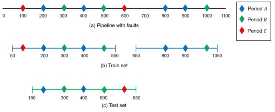
Figure 1.
Example of training and test sets. (a) Pipeline with faults, (b) Train set, and (c) Test set.
Figure 1b shows how the training set is constructed while using the Dynamic segmentation. The segmentation only takes into account faults in period A (blue). Ergo, we obtain two segments: the first segment starts at 50 m and ends at 550 m from the start of the line. The second segment spans between 650 and 1150 m. When we calculate the FaultCount feature of the two segments, we only consider faults from period A—blue diamonds. Therefore, the value of this feature is two in both segments. When calculating the label, only faults in period B (green diamonds) are examined. Accordingly, we get a label of two in the first segment and a label of one in the second segment.
Finally, Figure 1c illustrates the test set construction. Here we once again use Dynamic segmentation to build the segments, and this time consider only green diamonds, which depict failures in period B. The result is a single segment that begins at 150 m and ends at 650 m. The FaultCount feature is counted using faults from period B during testing, so its value is 2. The label is computed as the number of faults in period C (red diamond), which is 1.
An alternative way to split the data could be dividing the segments to two unequal sets: 85% of the segments are used for the training set and 15% for test. In this paper, we did not adopt this approach, since, when using a training set to learn a fault prediction model, there is an implicit assumption that the training set and the test set are taken from the same distribution. This assumption explains why by learning from the training set (in our case, historical segments of the waterline) we can predict the label of a new segment in the test set. When using the same segments for training and test (but in different time periods) we guarantee this assumption. However, in the alternative approach, when dividing the segments to two sets, it is more probable that the test set distribution will be slightly different than the training set.
Objective description: suppose a water utility that wants to employ a proactive maintenance strategy in its waterline network during the upcoming T time units. That is, the utility desires to prevent futuristic faults in its network by replacing in advance parts of the network that are prompt to fail during this time. This requires the utility to predict the areas where failures are likely to occur, and to decide which of these areas are most profitable to replace given a certain replacement budget. The mechanism that we propose can be utilized in order to acquire those predictions. The utility should make use of the logs of past faults that occurred within the network during the most recent 2T time units, and divide those logs into two parts, such that each of them would span T time units. Those two parts would correspond to the time periods A and B in our definition, and the future would represent period C. A prediction algorithm can be trained while using periods A and B, by finding the relation between faults in those two consecutive periods. Once the algorithm is trained, it can be inputted the faults from period B to predict faults in period C—the future. This would result in prediction that takes into account the most recent faults and, therefore, should be accurate because the connection between faults in consecutive periods has been learned. Those predictions can then be used to decide which segments should be replaced.
2.3. Prediction Algorithms
The data driven prediction algorithms we use utilize two kinds of features: (1) raw data features and (2) features extracted based on Mekorot experts’ knowledge. In the next list, we mention, for each feature, whether it is raw or given by experts.
- FaultCount—for the training set, this is the number of faults in period A, for the test set this is the number of faults in period B (raw).
- Age—the time difference in years between 1 January 2020 and the installation date of the segment (raw).
- LifeExpectancy—estimation of experts to the lifetime of the segment, according to its material (expert).
- TimeCondition—a binary measure. If the segment is made of concrete and was manufactured after 1965, or if it is made of steel and was manufactured between 1988 and 1995, the score is 1. Otherwise, the score is 0 (raw).
- MaterialScore—score given by experts according to the material of the segment (expert).
- AgeScore—score given according to the ratio between Age and LifeExpectancy (expert).
- LengthScore—score given according to the length of the segment and according to its FaultCount (expert).
Flowing water features, such as velocity, pressure, and acid gas content, and features about underground environment, such as temperature, could also contribute a lot to the pipe faults. Unfortunately, this type of data has not been available by Mekorot.
There are many of-the-shelf prediction algorithms [23] that could be applied in our case. One of the most popular ones is Linear Regression [24]. This model assumes a linear relationship between the features of the segments’ and the number of faults that they have. Mathematically, the following formula is assumed: , where are the features of a segment, y is the number of faults the segment has, are coefficients, and is a random variable that describes the error, which is the difference between the real value and the outcome of the linear function. This variable is assumed to have a mean of zero and constant variance. Given the train set, the training of the algorithm is done by calculating the coefficients in a way that minimizes the sum of squared errors between the real and resulting y values. Once the coefficients are calculated, the model can be easily used to predict the number of faults in a segment by inserting its features to the resulting formula.
Random Forest [25] is another well-known prediction algorithm, which is an ensemble-based machine learning algorithm used for both regression and classification. Ensemble algorithms are those that use multiple predictors and combine their results. In the case of Random Forest, it uses bootstrapping to take the average of the predictions of several decision trees. One of the main advantages of Random Forest is resistance to overfitting because of the large number of trees.
There are many of-the-shelf prediction algorithms [23]. Here, we list the algorithms we evaluated to predict the number of faults in a segment.
- Basic—Linear Regression algorithm using the MaterialScore, AgeScore and LengthScore features.
- Full—Linear Regression algorithm using all the features explained above.
- RF Regression—Random Forest Regression algorithm using all of the features explained above.
3. Evaluation
In this section, we describe the evaluation process (Section 3.1) and results (Section 3.2) of the suggested segmentation methods and prediction algorithms over real-world data.
3.1. Experimental Setup
In Section 3.1.1, we describe the data preparation for the experiments. In Section 3.1.2, we present a rule-based prediction algorithm that is currently used in Mekorot. In Section 3.1.4, we describe how we divided the data to training and test sets. Subsequently, in Section 3.1.3, we explain the metrics that are used to evaluate the prediction algorithms.
3.1.1. Data Description and Preprocessing
We evaluated our prediction models on real-world data: the water network of Israel, obtained by Mekorot, the national water main company of Israel. These data include the next main sources:
- Geographic Information System (GIS). Mekorot’s GIS contains geographic data about all the waterlines in Mekorot’s network. Lines are partitioned to sub-lines, where each sub-line is associated with information about its material.
- Systems—Applications—Products in data processing (SAP). Mekorot’s SAP contains (1) operational characteristics of the different water pipes. This includes the age of each water pipe. (2) Water pipe failure reports from June 2016 to December 2019.
Every waterline in the GIS is uniquely identified by a line ID and every line is partitioned into sub-lines that are uniquely identified by a sub-line ID. The GIS includes information regarding the material and the start and end coordinates of each sub-line in every waterline. However, the data in SAP include information regarding the age of only the line ID rather than sub-line ID. Therefore, we associated each sub-line with the age of the line that contains it. In the water pipe failure reports, failures are associated with a line ID and the coordinates of the fault. We used the ArcMap GIS software to find the sub-line that matches the fault coordinates. Faults without any input coordinates (less than 4% of the faults) were dropped. Faults whose input coordinates is further than 400 m to the nearest segment were also removed.
As a pre-process to our experiments, we filtered out some of the faults and waterlines data, as instructed by experts from Mekorot. Out of a total of 3682 waterlines:
- 13 waterlines were removed because they lacked information about their construction type.
- An additional 247 waterlines were removed because the given coordinates of their segments could not be connected to each other.
Finally, 3423 pipes remained. Among the 5412 faults between June 2016 and October 2019:
- 32 were discarded because they lacked information about the pipe they occurred in.
- 1395 were discarded because they lacked information either about the quality of the measurement or about whether it was an burst/leakage.
- 1235 were discarded because they were not bursts or leakages.
- 127 were discarded because of low quality or calculation errors.
- 40 were discarded because they lacked information about their location in the pipes.
- 276 were discarded because they contained an invalid line id.
- 63 were discarded because their location was invalid.
Finally, 2244 faults remained.
3.1.2. Rule-Based Model
We compare them to a rule-based model proposed by experts in Mekorot, based on their rich experience in order to evaluate the proposed data-driven prediction algorithms. Mekorot Model (hereinafter MM) is a model used by Mekorot to assess the need to replace a given waterline segment. The current use case of MM is that a waterline engineer suggests to replace a segment of a waterline and the MM helps to inform the decision makers regarding whether to approach this request or not. MM is implemented as a set of rules. Given a candidate waterline, it is characterized by a set of features and MM computes a score between 0 to 100 for that segment. This score represents the need for replacing the pipe segment, where 100 means urgent need for replacement and 0 means no need to replace the line segment at all. MM considers seven features:
- Construction Type Score: a score that is based on the material of the waterline.
- Workload Score: the ratio of the operational pressure of the waterline divided by its nominal pressure.
- Age Score: the waterline’s age divided by its life expectancy. A waterline’s life expectancy is set according to the type of the waterline. The range of this feature is [0,1].
- Faults to Length Score: the number of leakages and bursts in the segment to be replaced in the last 5 years divided by the length of that segment. The exact way the Length feature is computed is as follows. Let ReplacementLength be the length of the segment to be replaced, and let FaultCount be the number of faults in that segment in the past five years. The LengthRatio is defined as . The Length Score feature is computed as .
- Consumers Score: the population amount at the pipe’s distribution region, the consumption type, whether its agricultural or domestic, and the average flow rate.
- Potential Damage Score: the potential damage fix cost and potential cost of the compensation to the consumers and the land owners.
- Analysis Score: experts’ recommendation.
The value of each feature is normalized to be between 0 and 100, and the overall value of a given segment is a weighted sum of these features, where the weights of Type, Workload, Age, Length, Consumer, Damage, and Analysis features are 0.25, 0.15, 0.05, 0.30, 0.10, 0.05, and 0.10, respectively.
These seven features are divided into two groups. The first group, consisting of Construction Type, Workload, Age, and Faults to Length, is used to estimate the probability of a failure (leakage or break) of a pipe line. The second group of features, consisting of Consumers, Potential Damage, and Analysis, is used to estimate the expected damage of a failure in the given pipeline. Because the scope of this work focuses on fault prediction rather than impact estimation, we focus on the first group of features. Additionally, we did not have access to the data required to compute the Workload feature, and therefore we did not use this feature. Thus, MM failure prediction model we used is computed, as follows: , where the division by 0.6 is done in order to obtain a normalized value between 0 and 100.
Because we aim to predict the number of faults in a pipe, as the proposed data-driven algorithms do, a value between 0 and 100 is not appropriate. Therefore, we performed the following normalization. Let and be the average and standard deviation of the number of faults in period B, and let and be the average and standard deviation of the scores that were outputted by Mekorot’s model for segments in period B, we set the normalized Mekorot score to be:
where Y is the new normalized Mekorot score and X is the previous Mekorot score. The logic behind this normalization is to force the average and standard deviation of the normalized Mekorot score to be the same as the average and standard deviation of the number of faults, respectively.
3.1.3. Metrics
The prediction algorithms predict the number of faults in period C. We evaluated the algorithms by comparing the predicted value to the actual number of faults in period C. We measured the error while using the following metrics:
RMSE: the first metric is Root Mean Squared Error (RMSE). This measure is used to calculate the difference between the prediction and the actual number of faults. RMSE is calculated by subtracting the predictions from the actual faults of each segment, summing up the squares of all the results and taking the root of it. means that the prediction is exactly as the actual number of faults for all cases. The larger the RMSE, the worse the prediction.
Conover [26]: this is a ranking-based metric, which measures the correlation between the rankings of the actual and predicted fault counts of each segment. First, the segments receive a ranking based on their actual fault counts. Afterwards, the segments receive a second ranking, by sorting them according to their predictions, and assigning the above-mentioned ranks according to the segments’ positions in the sorted list. The resulting metric is average of absolute differences between the two ranks of each segment. Assume, for instance, that the actual fault counts of six segments are [1,3,5,6,3,3], and the predicted number of faults are [2,4,6,6,9,3]. The ranking according to the actual faults is [0,2,4,5,2,2]. Thus when we sort the segments by the predictions and distribute those same ranks, we would obtain the ranks [0,2,2,4,5,2]. The absolute differences between those two rankings are [0,0,2,1,3,0], and the final score is the average of those differences, which is 1.
Kendall’s Tau [27]: this is also a ranking-based metric, which measures the correlation between the actual and predicted number of faults for each possible pair of segments. A pair of segments is considered concordant if both the actual and the predicted number of faults in one segment are larger than in the other. A pair is considered discordant if one segment has more actual faults than the other, but the prediction of the second is higher than the first. The metric measures the number of concordant pairs (P), the number of discordant pairs (Q), the number of pairs with ties in the prediction (U) and the number of pairs with ties in the actual number of faults (T). The score is calculated as: . Values of this metric that are close to 1 indicate strong agreement between reality and prediction, values close to −1 indicate strong disagreement, while values around 0 indicate that there is no correlation between them. Unlike the other metrics, here a higher result would mean a better prediction.
3.1.4. Training and Test Sets
A learning prediction algorithm should include a training set and a test set, as mentioned in Section 2.2. To this end the data is divided to three time periods, 13 months each: (A) 1 June 2016 to 30 June 2017, (B) 1 July 2017 to 31 July 2018, and (C) 1 August 2018 to 31 August 2019. To evaluate the performance of the different prediction algorithms on the different segmentation methods, we varied (1) the training data and (2) the test set, as follows:
Training set
- 2+ faults: we considered only the segments with at least two faults in period A.
- (a)
- For the Fixed segmentation, we simply filtered the segments with at least two faults in period A, and remained with 99 segments.
- (b)
- The Dynamic segmentation ensures by its definition that all of the resulting segments contain at least two faults in period A. In total he had 102 segments in this segmentation method.
- ALL segments: using all of the waterline data for the training set:
- (a)
- In the fixed segmentation we considered all the segments (22,516 segments).
- (b)
- For the dynamic segmentation: we extended the segmentation to also include segments with less than two faults. To do this, we generated a segment from all groups of faults that occurred within 300 m of each other: even groups that only contained a single fault. Afterwards, for the remaining parts of waterlines that still did not belong to any segment, we divided them to fixed size segments of 293 m each, which was the average length of the rest of the segments. In total, we had 29,620 segments.
Test set
- 2+ faults: we only filtered the segments with at least two faults in period B. In total, we had:
- (a)
- 99 segments in the fixed segmentation.
- (b)
- and 104 in the dynamic segmentation.
The reason that we used only segments with two or more faults in the test set is because the overwhelming majority of segments did not have any faults in the third period. Because most of our metrics are ranking-based, they are not very suitable in situations where there are many ties in the labels. For that reason, we filtered the segments with at least two faults in period B, because the data distribution in those segments in period C was more balanced.
Table 1 summarizes the number of segments.

Table 1.
Summary of the number of segments in the training and test sets.
3.2. Results
This section presents the results of the experiments. In Section 3.2.1, we present the result of the prediction algorithms. In Section 3.2.2, we examine the influence of the size of the training set on the accuracy of the prediction models. Finally, In Section 3.2.3, we examine the impact of geographical features on the accuracy of the prediction model.
3.2.1. Methods Evaluation
Figure 2, Figure 3 and Figure 4 present the results of the RMSE, Conover, and Kendall’s Tau metrics for the regression-based algorithms and for Mekorot’s expert-based model. Each chart represents a single metric, and it displays the results for that metric of all algorithms in each of the four segmentation methods. The x-axis corresponds to the different prediction algorithms and the y-axis shows the value of the metric. Recall that, for the RMSE and Conover metrics, lower values imply better results, while, for the Kendall’s Tau metric, higher values mean better results. The segmentation methods are not comparable, since the test set in each one contains different segments and a different amount of segments. We would like to provide conclusions regarding (1) the comparison between the regression based method and Mekorot’s model and (2) the impact of the training data on the accuracy of the prediction.
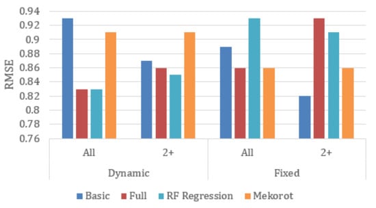
Figure 2.
Root Mean Squared Error (RMSE) metric for the fixed and dynamic segmentation methods (the lower the better).
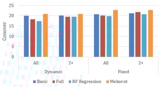
Figure 3.
Conover metric for the fixed and dynamic segmentation methods (the lower the better).
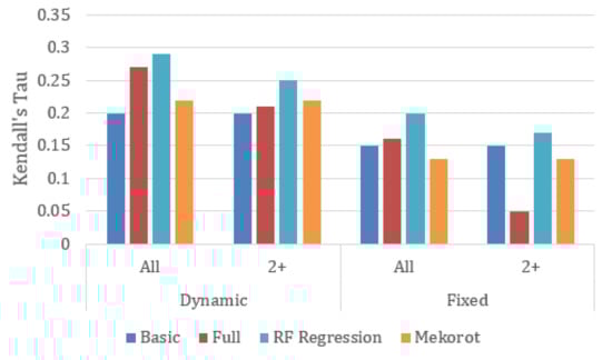
Figure 4.
Kendall’s Tau metric for the fixed and dynamic segmentation methods (the higher the better).
RMSE: we can see that in the Dynamic segmentations Full and RF Regression have the best performance, both improving Mekorot by 8.7% in the Dynamic All segmentation, as well as, respectively, 5.4% and 6.6% in the Dynamic 2+ segmentation. However, in the fixed segmentations, Mekorot outperforms them, providing an improvement of 7.5% over Full in Fixed 2+ segmentation, and improvements of 7.5% and 5.4% over RF Regression in Fixed All and Fixed 2+, respectively. Full performs best when trained using all the data, while Basic provides better results when only trained using segments with two or more faults.
Conover: we can see that all regression-based algorithms outperform Mekorot. The improvements obtained by Basic over Mekorot are in the range of 4.7–8.6%, those obtained by Full are in the range of 4.3–14.2%, and those of RF Regression are in the range of 8.6–19%. Additionally, training on all data slightly improves the performance of those algorithms.
Kendall’s Tau: RF Regression takes the lead in all four segmentation methods, showing improvements in the range of 13.6–53.8% over Mekorot, and training on all the data improves the accuracy of all regression-based algorithms.
We can conclude that:
- In all configurations at least one regression-based model outperforms Mekorot, improving its RMSE resulting by at least 5%, the Conover result by at least 4%, and the Kendall’s Tau result by at least 13%.
- In the Dynamic segmentation, Full and RF Regression have better results than Mekorot, but it seems that mostly RF Regression performs the best, with an improvement of up to 8.7& in the RMSE metric, up to 14.3% in Conover, and up to 31.8% improvement in the Kendall’s Tau metric.
- Full and RF Regression should be trained with all data, while Basic should be trained while using only segments with 2+ faults.
3.2.2. The Impact of the Training Set Size
In machine learning algorithms, usually, the larger the training set the more accurate the model. In this section, we would like to examine this common sense in our domain. To this end, we enriched the training set in two ways as follows:
- We split our data of past faults into four periods of 10 months each, unlike the usual division to three periods of 13 months. By doing so, we were able to use two periods, A and B, each one with 10 months, as the training set and thereby increasing the training set size from 29,943 segments to 60,508 segments. Afterwards we inserted the faults from period C into the trained prediction model to predict faults in period D, and finally compare them to the actual amount of faults in that period (20 months).
- We split the data into four periods, as in the previous experiment, but we trained the model with a total of 30 months: the 20 months from the last experiment, and an additional 10 that we obtained by overlapping periods A and B: we took the last five months from period A and the first five months from period B. In total, the training set consisted of 90,451 segments. Subsequently, we tested the model using periods C and D, as described above (30 months).
We experiment on the RF Regression prediction algorithm and on Mekorot in a configuration of a dynamic segmentation, where ALL the data was trained. We compared the proposed two ways of enriching the training set (20 months, 30 months) to a simple training set of 10 months (10 months), and tested all options on the same test set of 10 months. Results are shown in Table 2.
Table 2.
RF Regression with different training set sizes.
The table shows the metrics for each training set size of each algorithm. Values in bold indicate the best metric value for a give algorithm. We can observe that increasing the size from 10 months to 20 months has a positive effect on the RF Regression algorithm. Increasing from 20 months to 30 has somewhat of an ambiguous impact on the results, due to the overlap in the training periods. We conclude that increasing the training set size is beneficial for the prediction, but overlapping training periods is not recommended.
3.2.3. The Impact of Geographical Features
In this sectionm, we would like to examine the impact of geographical features on the accuracy of the prediction model. The geographical features we add to each segment are:
- The number of faults in the entire waterline in which the segment belongs to (Fault Count).
- The Euclidean distance between the segment to the closest fault, as well as the number of fault occurrences in a certain radius from the segment (Fault Distance).
- The number of GIS subsegments that exist in the segment (GIS segments).
We run experiments on the RF Regression prediction algorithm, as well as Mekorot’s model, in a configuration of a dynamic segmentation, where ALL the data was trained. We tried the RF Regression algorithm in five different configurations: as-is (Normal), with the addition of each of the above three features separately (Fault Count, Fault Distance, GIS Segments), and with all of them combined (All). The results of the experiment are given in Table 3.
Table 3.
RF Regression with geographical features compared to Mekorot.
The table displays the results of the three metrics for each configuration of RF Regression and of Mekorot. Values that are in bold are the best result among the five feature configurations for each metric. We can see from the table that, for the RF Regression algorithm, we generally notice a negative impact on the results from the additions. We therefore conclude that geography-related features are generally not very useful for the prediction.
4. Discussion
In this section we would like to discuss some of the limitations of our proposed methodology, namely the lack of features and the imbalanced dataset.
There is wide variety of variables that might affect faults in pipes, such as the diameter of the pipe, the water pressure, rainfall at the pipe area, the soil type, and many other possibly important features. Unfortunately, those features were not available to us, so we were unable to utilize them with the prediction algorithms. It is our hope that Mekorot would start collecting this kind of data, so that we can use it in the future.
In addition, in this paper we focused on burst or leakage faults in pipes. Predicting faults that result due to reasons other than bursts or leakages was not within the goals of our paper. Bursts and leakages result from natural reasons, such as aging of the pipes or bad materials. Other failures, such as those that occur due to the pipes being hit by an external object, are not something that can be predicted and, for that reason, we intentionally filtered out those kinds of faults.
Another aspect that we would like to point out is that the overwhelming majority of segments in our network did not experience a single fault during the observed time range (June 2016–December 2019). A prediction model that was trained with such an imbalanced dataset will have a much higher tendency to predict very small fault counts for segments. This could impair the quality of the prediction. A natural way to deal with this issue would be to increase the size of the dataset by collecting faults over a larger time frame. In addition, several algorithms have been proposed that aim to balance the data using under-sampling or over-sampling techniques [28,29]. Our solution to the problem was to filter segments that had a value of two or more in the FaultCount feature. This technique relied on the assumption that fault occurrences in a certain period increased the probability for fault occurrences in the next period. Indeed, this methodology increased the balancing of the predictions of our algorithms.
5. Conclusions
We discussed the need to employ a proactive maintenance strategy in order to reduce the costs that are associated with maintaining waterline networks. For that goal, we proposed two segmentation algorithms to split waterlines to segments, and three data-oriented prediction algorithms to predict faults in each segment. We compared these algorithms to an expert rule-based decision model while using the common metrics RMSE, Conover, and Kendall’s Tau. The data driven algorithms provided better results than the expert rule-based model by at least 5%, 4%, and 13% in those three metrics, respectively. In addition, it can be concluded that these algorithms provide better results when they are trained with more data, and that enhancing these algorithms with geography-related features does not improve their accuracy, as it was expected by [1].
Future work will focus on developing more sophisticated prediction algorithms, including Baysian belief networks and deep neural networks. In addition, we want to investigate how to utilize predictions of failures in waterlines in order to propose a cost-effective maintenance strategy. By doing this, we will be able to recommend the segments that are most profitable for replacement based on factors, such as failure probability, replace cost, and failure cost.
Author Contributions
Conceptualization, All.; methodology, A.G. and M.K.; software, A.G.; validation, D.F.-H.; formal analysis, A.G. and M.K.; investigation, All; resources, S.H.; data curation, A.G. and M.K.; writing–original draft preparation, A.G. and M.K.; writing–review and editing, All.; visualization, All; supervision, A.G. and M.K.; project administration, M.K.; funding acquisition, S.H. All authors have read and agreed to the published version of the manuscript.
Funding
This research was funded by Mekorot company and by ISF grant No. 1716/17.
Conflicts of Interest
The authors declare no conflict of interest.
References
- Scheidegger, A.; Leitão, J.; Scholten, L. Statistical failure models for water distribution pipes—A review from a unified perspective. Water Res. 2015, 83, 237–247. [Google Scholar] [CrossRef] [PubMed]
- Rizzo, P. Water and Wastewater Pipe Nondestructive Evaluation and Health Monitoring: A Review. Adv. Civ. Eng. 2010, 2010, 818597. [Google Scholar] [CrossRef]
- Liu, Z.; Kleiner, Y.; Rajani, B.; Wang, W. Condition Assessment Technologies for Water Transmission and Distribution Systems; Tech. Rep.; U.S. Environmental Protection Agency: Washington, DC, USA, 2012. [Google Scholar]
- Kleiner, Y.; Rajani, B. Comprehensive review of structural deterioration of water mains: Statistical models. Urban Water 2001, 3, 131–150. [Google Scholar] [CrossRef]
- Friedl, F.; Möderl, M.; Rauch, W.; Schrotter, S.; Liu, Q.; Fuchs-Hanusch, D. Failure Propagation for Large-Diameter Transmission Water Mains Using Dynamic Failure Risk Index; World Environmental and Water Resources Congress: Milwaukee, WI, USA; American Society of Civil Engineers (ASCE): Reston, VA, USA, 2012; pp. 3082–3095. [Google Scholar]
- Kleiner, Y.; Rajani, B. Comparison of four models to rank failure likelihood of individual pipes. J. Hydroinform. 2011, 14, 659–681. [Google Scholar] [CrossRef][Green Version]
- Eisenbeis, P.; Rostum, J.; Le Gat, Y. Statistical models for assessing the technical state of water networks: Some european experiences. In Proceedings of the Annual Conference American Water Works Association, Chicago, IL, USA, 20–24 June 1999; p. 13. [Google Scholar]
- Røstum, J. Statistical Modelling of Pipe Failures in Water Networks. Ph.D. Thesis, University of Science and Technology, Trondheim, Norway, 2000. [Google Scholar]
- Xu, Q.; Chen, Q.; Li, W.; Ma, J. Pipe break prediction based on evolutionary data-driven methods with brief recorded data. Reliab. Eng. Syst. Saf. 2011, 96, 942–948. [Google Scholar] [CrossRef]
- Song, H.; Du, S.; Wang, R.; Wang, J.; Wang, Y.; Wei, C.; Liu, Q. Potential for Vertical Heterogeneity Prediction in Reservoir Basing on Machine Learning Methods. Geofluids 2020, 2020, 3713525. [Google Scholar] [CrossRef]
- Zhang, Q.; Wei, C.; Wang, Y.; Du, S.; Zhou, Y.; Song, H. Potential for prediction of water saturation distribution in reservoirs utilizing machine learning methods. Energies 2019, 12, 3597. [Google Scholar] [CrossRef]
- Wang, R.; Dong, W.; Wang, Y.; Tang, K.; Yao, X. Pipe failure prediction: A data mining method. In Proceedings of the 2013 IEEE 29th International Conference on Data Engineering (ICDE), Brisbane, Australia, 8–11 April 2013; pp. 1208–1218. [Google Scholar] [CrossRef]
- Giraldo-González, M.M.; Rodríguez, J.P. Comparison of Statistical and Machine Learning Models for Pipe Failure Modeling in Water Distribution Networks. Water 2020, 12, 1153. [Google Scholar] [CrossRef]
- Berardi, L.; Giustolisi, O.; Kapelan, Z.; Savic, D.A. Development of pipe deterioration models for water distribution systems using EPR. J. Hydroinform. 2008, 10, 113. [Google Scholar] [CrossRef]
- Snider, B.; McBean, E.A. Improving Urban Water Security through Pipe-Break Prediction Models: Machine Learning or Survival Analysis. J. Environ. Eng. 2020, 146, 04019129. [Google Scholar] [CrossRef]
- Alizadeh, Z.; Yazdi, J.; Mohammadiun, S.; Hewage, K.; Sadiq, R. Evaluation of data driven models for pipe burst prediction in urban water distribution systems. Urban Water J. 2019, 16, 136–145. [Google Scholar] [CrossRef]
- Chen, T.J.; Guikema, S. Prediction of water main failures with the spatial clustering of breaks. Reliab. Eng. Syst. Saf. 2020, 203. [Google Scholar] [CrossRef]
- Scholten, L.; Scheidegger, A.; Reichert, P.; Mauer, M.; Lienert, J. Strategic rehabilitation planning of piped water networks using multi-criteria decision analysis. Water Res. 2014, 49, 124–143. [Google Scholar] [CrossRef] [PubMed]
- Poulton, M.; Le Gat, Y.; Brémond, B. The impact of pipe segment length on break predictions in water distribution systems. Strategic Asset Management of Water Supply and Wastewater Infrastructures; IWA Publishing: London, UK, 2009; p. 419. [Google Scholar]
- Jiang, Y.; Cukic, B.; Ma, Y. Techniques for evaluating fault prediction models. Empir. Softw. Eng. 2008, 13, 561–595. [Google Scholar] [CrossRef]
- Schwabacher, M. A survey of data-driven prognostics. In Infotech@ Aerospace; American Institute of Aeronautics and Astronautics: Arlington, VA, USA, 2005; p. 7002. [Google Scholar]
- Salfner, F.; Lenk, M.; Malek, M. A survey of online failure prediction methods. ACM Comput. Surv. (CSUR) 2010, 42, 1–42. [Google Scholar] [CrossRef]
- Baldi, P.; Brunak, S.; Chauvin, Y.; Andersen, C.A.; Nielsen, H. Assessing the accuracy of prediction algorithms for classification: An overview. Bioinformatics 2000, 16, 412–424. [Google Scholar] [CrossRef]
- Shi, F. Data-Driven Predictive Analytics for Water Infrastructure Condition Assessment and Management. Ph.D. Thesis, University of British Columbia, Vancouver, BC, Canada, 2018. [Google Scholar]
- Liaw, A.; Wiener, M. Classification and regression by randomForest. R News 2001, 2, 18–22. [Google Scholar]
- Iman, R.L.; Conover, W.J. A distribution-free approach to inducing rank correlation among input variables. Commun. Stat. Simul. Comput. 1982, 11, 311–334. [Google Scholar] [CrossRef]
- Maurice, K. A new measure of rank correlation. Biometrika 1938, 30, 81–89. [Google Scholar]
- Chawla, N.V.; Bowyer, K.W.; Hall, L.O.; Kegelmeyer, W.P. SMOTE: Synthetic minority over-sampling technique. J. Artif. Intell. Res. 2002, 16, 321–357. [Google Scholar] [CrossRef]
- Tahir, M.A.; Kittler, J.; Yan, F. Inverse random under sampling for class imbalance problem and its application to multi-label classification. Pattern Recognit. 2012, 45, 3738–3750. [Google Scholar] [CrossRef]
Publisher’s Note: MDPI stays neutral with regard to jurisdictional claims in published maps and institutional affiliations. |
© 2020 by the authors. Licensee MDPI, Basel, Switzerland. This article is an open access article distributed under the terms and conditions of the Creative Commons Attribution (CC BY) license (http://creativecommons.org/licenses/by/4.0/).