The Effect of Best Crop Practices in the Pig and Poultry Production on Water Productivity in a Southern Brazilian Watershed

Abstract

This study analyzes the relation between Brazilian broiler and pig production and water productivity using recently developed reference guidelines on water footprinting for livestock production systems and supply chains. Different rainfed crop arrangements, in different scenarios and producer regions in Brazil, were assessed. Water productivity of broiler feed consumption ranged from 0.63 to 1.38 kg per m³ water input to rainfed summer maize (safra) and from 1.20 to 2.21 kg per m³ water input to winter maize (safrinha) while it ranged from 0.28 to 0.95 kg per m³ water input to rainfed soy. For pig feed consumption, rainfed maize ranged from 0.68 to 1.49 kg per m³ water input (safra) and from 1.30 to 2.38 kg per m³ water input (safrinha) while it ranged from 0.30 to 1.03 kg per m³ water input to rainfed soy. A potential amount of water saving of 0.0336 km³ year⁻¹ and 0.0202 km³ year⁻¹ could be attained for producing broiler and pig feed, respectively, depending on the crop rotation and producer region. The results showed that the evapotranspiration of animal feed production represents more than 99% of the total water consumption for broiler and pig production in the study area. The implementation of best crop practices resulted in higher water productivity values of chicken and pork meat and also improved the rainfall water-saving in comparison to conventional agriculture. Hence, the water productivity of the animal production chain in tropical regions demands a close relation to agriculture in order to attain a better understanding and improvement of rainfall water productivity for animal feed production.

1. Introduction

Water is a crucial resource in agriculture [1], which stands out as the major user of water, accounting for about 70% of the world’s freshwater withdrawal [2]. Freshwater demands are increasing worldwide and water scarcity is becoming a threat to the sustainable development of human society [3]. There is a need for widely recognized frameworks to assess the performance of e.g., livestock and livestock products in order to mitigate negative impacts on water resources [1]. Progress has been made recently in the field of assessing water demand in agriculture, and its related impacts on water scarcity, through the development of ISO 14046:2014 [4] “Environmental management—water footprint—principles, requirements and guidelines” and ISO/TR 14073:2016 [5] “Environmental management—water footprint—illustrative examples on how to apply ISO 14046”. Recently, the Livestock Environmental Assessment and Performance Partnership (LEAP)—Food Agriculture Organization (FAO) organized a Technical Advisory Group (TAG) on water footprint. Last year, the TAG published the guidelines “Water use in livestock production systems and supply chain” [1]. These guidelines complement the ISO assessment framework with water productivity and water scarcity impact assessment methods.

The FAO Guidelines aim to improve the environmental sustainability of livestock supply chains through better methods, metrics, and data for the assessment of water use in livestock production systems and supply chains in order to quantify the potential environmental impacts related to water scarcity and to identify actions for improvement in water management. As the first guidelines, they require validation of the proposed methodology. Countries’ studies are a way of doing this validation.

According to the Brazilian National Water Agency [6], because of the highest availability of fresh water in the world, Brazil has an apparent abundance of water for supplying all water demands in the country. However, the water resources are distributed unevenly in the territory, spatially and temporally. Water crises due to changes in rainfall patterns stemming from extreme events, as several droughts pointed out by Cunha et al. [7], Gutiérrez et al. [8], Coelho et al. [9], and Marengo et al. [10] cause high economic, social and environmental losses in the whole country.

The pressure on rainfed agriculture, which accounts for 60% of the global food output [11] and is directly dependent on rainfall and runoff patterns, becomes higher worldwide due to climate change effects [12]. On the global scene, a large portion of the water consumed by crops—an estimated 80%—comes directly from rainfall that infiltrates into the soil and forms soil moisture in the root zone which is eventually transpired or evaporated (green water) [11,13,14]. According to Hoff et al. [15], global green water used in the world crop production is about 4–5 times greater than consumptive blue water (irrigation) use. Considering rainfed agriculture as the dominant crop and forage production system throughout the world, the stability of food and fiber production requires that we increase green water productivity [16].

Rainfed agriculture in Brazil plays an important economic and social role, being cultivated in 97% of the municipalities. However, between 2013 and 2017, water for agricultural production exceeded the rainfall water available by 37% [17]. Empinotti [18] concluded consequently that since most Brazilian crop and livestock productions are based on rainfed systems, green water management should be a focus to improve water productivity.

In order to develop strategies to adapt agricultural methods to changes in regional water availability, it is necessary to know how much water is currently being used on farms for agricultural production and products of animal origin [19]. Water productivity is the ratio of the net benefits to the amount of water consumed to produce those benefits. It includes all direct (operational use) and indirect (supply chain use) water flows. The water productivity assessment can help farmers to optimize the water flows in their farms and enhance water use through agronomic measures and farm management [1]. The water productivity assessment on farm-scale not only captures the yield improvement in one specific field but can also be applied to the water value chain as an integrative indicator in order to measure enhanced use of water flows [20].

Recent studies addressed water productivity assessment of rainfed maize and soy based on evapotranspiration (ET) under different conditions [21,22] and for different regions of Nebraska in the USA [23,24], and Nigeria in Africa [25], where results of water productivity varied depending on the climate conditions and soil. In Brazil, Flach et al. [26] analyzed the water productivity of major Brazilian rainfed crops and observed the dominance and importance of rainfall as a resource for agriculture in Brazil.

The aim of this study was to evaluate water productivity indicators of broiler and pig production in a Southern Brazilian watershed according to the methodology proposed by the FAO [1]. Different rainfed crop arrangements in different yield scenarios considering less soil evaporation were assessed, which allowed us to learn how feed water productivity impacts the water productivity of chicken and pork meat.

This study is the first to apply the guidelines published by the FAO [1] for water productivity assessment on Brazilian livestock production. It aims to contribute to the knowledge related to water demand for animal production based on water productivity assessment and the importance of best practice implementation for raising water productivity of animal feed production in order to achieve a more sustainable production chain in Brazil.

2. Materials and Methods

2.1. General Approach

Water Productivity (WP) was calculated on farm-scale according to the FAO [1] for pig (WP_{indirect+direct,pig,Farm}) and broiler (WP_{indirect+direct,broiler,Farm}) production performed in the Lajeado Tacongava watershed in Southern Brazil for the year 2019. This study was focused on WP for purchased crops for animal feed. Summer and winter season maize crops, called safra and safrinha, respectively, and soybean produced in specific crop rotations were analyzed, considering the current yield. Potential strategies for raising water productivity, as higher yield and lower soil evaporation, were also analyzed. Evapotranspiration as indirect water consumption was considered to calculate feed water productivity (WP_{indirect,broiler,Feed}; WP_{indirect,pig,Feed}). The direct water consumptions were animal drinking (Q_{direct,pig,Animal}; Q_{direct,poultry,Animal}) and water for services (Q_{direct,pig,Housing}; Q_{direct,poultry,Housing}).

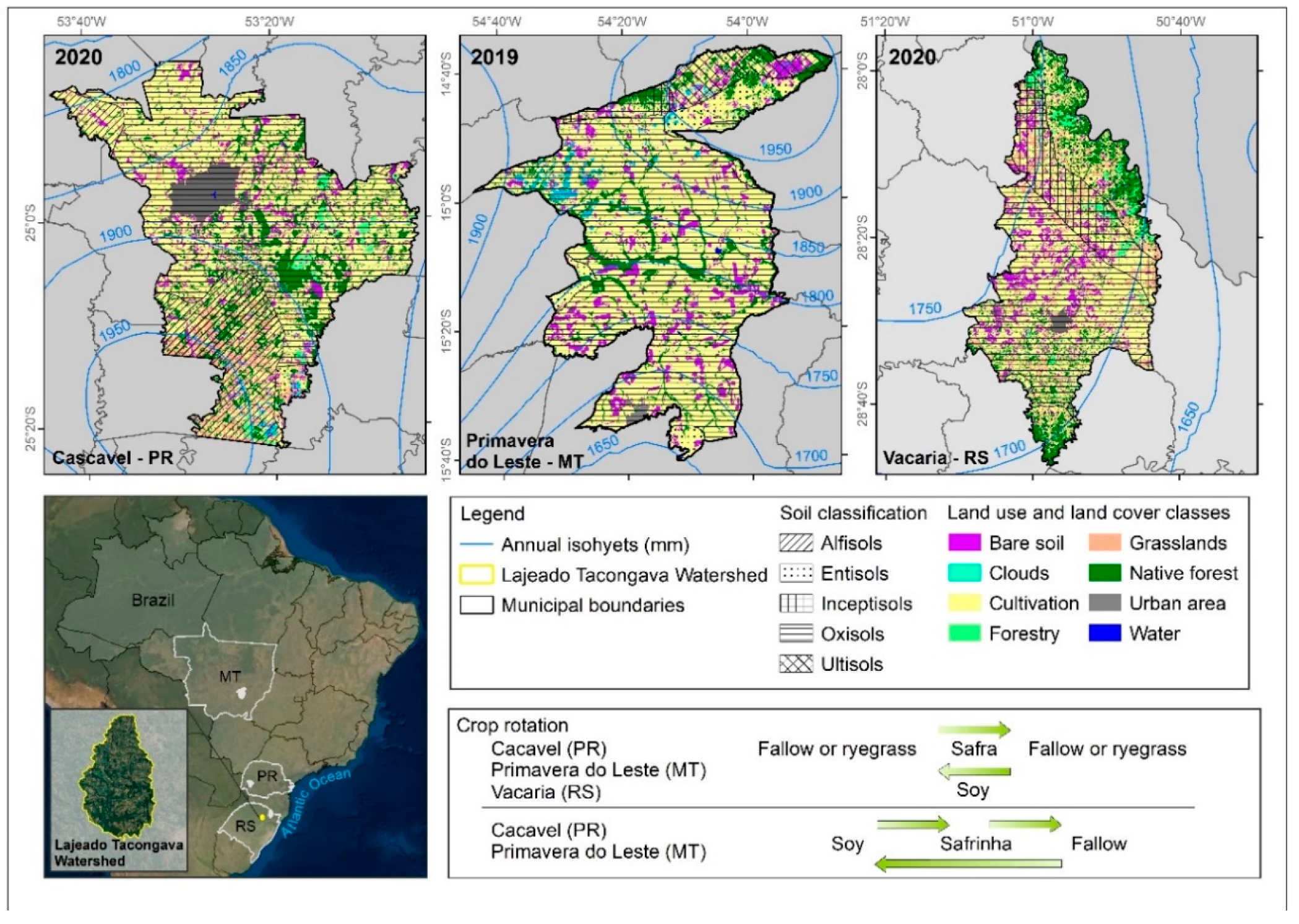
2.2. Study Area and Animal Production System Data

The study area was Lajeado Tacongava watershed (Figure 1) which is located in the Northeast region of the Rio Grande do Sul State, Southern Brazil. With an area of 149.78 km², the watershed is partially comprised of four cities with tradition in agriculture and livestock production: União da Serra, Serafina Correa, Montauri, and Guaporé. Farms with more than 50 fattening pigs and more than 1000 broilers were investigated. Criteria for farms selection were defined according to the environmental license classification [27] and economic viability. Figure 1 shows the location of farms in the watershed.

Between June 2019 and March 2020, we surveyed 78 farms (37 pig production and 41 poultry farming). Information related to farm-basic data (name, address, location, family workforce details, agricultural activities), environmental farm conditions (type of soil, water supply, water resources located on the farm, wastewater and solid waste management), and animal production features (current herd, the period of the production cycle, breeding systems, type of diet, initial and finishing weight) was collected.

The herd of pigs located on the farms within the Lajeado Tacongava watershed area ranged from 240 to 1150 head farm⁻¹cycle⁻¹, with a total herd of 55,071 head year⁻¹ for pig. For broiler, it ranged from 7500 to 85,000 head farm⁻¹cycle⁻¹ with a total herd of 6,108,600 head year⁻¹. Animal production is performed in a vertical integration system, where companies define initial and finishing animal weight according to the market demands. The first stages of the animals’ life are neither performed on the farms nor in the watershed. Piglets are born on a farm where they spend 28 days in the weaning stage and 35 days in a farm nursery stage until achieving the weight for starting the finishing stage in the last farm [28]. In this paper, the first stage of a pig’s life is called pig pre-chain. Broilers, as well, are born in a hatchery and after that, they are transported to the finishing farm. Figure 2 presents the stages, animal performance indicators, and water flows of the two animal production chains addressed in this study.

Broilers and pigs were considered mixed between males and females. The mortality rate for broilers was considered 3.5% per cycle [29] and for pigs, it was null in the finishing stage. Feed compositions for fattening broilers (64% maize and 27% soybean meal) [30,31] and pigs (75% maize and 25% soybean) [32,33] were established for different stages of growth as shown in the supplementary material (Table S1). Pig pre-chain feed composition for weaning (75% maize and 25% soybean) and nursery (54% maize and 24.3% soybean) were also defined [28]. Companies provide animal feed to the farms and diets are specific for each stage of life. For this reason, the daily amount of feed and the type of diet were standardized for all farms (Table S1).

Table 1. Input data standard for pig and broiler production—year: 2019.

Term	Data	Source
Broiler Production
Input
Number of Heads (head year−1)	6,108,600	Farm Survey
Initial weight (kg)	0.042	Cobb [31]
Production cycle (days)	42	Cobb [31]
Cycles (year)	6	Farm Survey
Output
Finishing weight (kg)	2.85	Cobb [31]
Mass output (kg CW head−1)	2.15	Cobb [31]; Embrapa [30]
Energy output (MJ kg−1)	4.98	USDA [34]
Revenues (R$ kg−1)	1.61	Embrapa [35]
Pig Production
Input
Number of Heads (head year−1)	55,071	Farm Survey
Initial weight (kg)	28.7	Agroindustry [33]
Production cycle (days)	105	Agroindustry [33]
Cycles (year)	3	Farm Survey
Output
Finishing weight (kg)	134.94	Agroindustry [33]
Mass output (kg CW head−1)	97.16	Embrapa [32]
Energy output (MJ kg−1)	15.72	USDA [34]
Revenues (R$ kg−1)	3.39	Embrapa [35]
Indirect Water
Input
Crop mean yield	t ha−1	IBGE [36]
Climate data	Parameters 1	INMET [37]
Climate classification	RS: Cfb; PR: Cfa; MT: Aw	Alvares et al., [38]
Type of soil	Clay	Streck et al., [39]; IBGE [40]
Direct Water
Input
Animal drinking	l head−1 day−1	Palhares [41]
Service—cleaning	l head−1 day−1	Drastig et al. [42]; FEPAM [43]
Service—cooling	l head−1 day−1	Drastig et al. [42]

CW: carcass weight; R$: Brazilian currency (real); RS: Vacaria (Rio Grande do Sul State); PR: Cascavel (Paraná State); MT: Primavera do Lesta (Mato Grosso State); ¹ precipitation (mm), minimum and maximum temperature (°C), sunshine hours (h), relative humidity (%), and wind speed (km h⁻¹).

shows the input data sources to calculate the water productivity indicators.

2.3. Calculation of Water Productivity

WP was calculated for broilers in the fattening stage (WP_{indirect+direct,broiler,Farm}) and pigs (WP_{indirect+direct,pig,Farm}) for pre-chain and fattening production stages accounting for direct and indirect water inflows, according to the FAO [1] and presented in Section 2.1.

The boundaries of the system were cradle-to-farm gate which involved feed and meat production at farm level. This study applied a bottom-up approach where farm specific data was used to calculate a detailed WP. In this study, WP was calculated in three references units in order to increase comparability with other studies. They were expressed on a mass basis (WP_{indirect+direct,broiler,Mass,Farm} (Equation (1)); WP_{indirect+direct,pig,Mass,Farm} (Equation (2))) (kg Carcass Weight (CW) m⁻³), food energy basis (WP_{indirect+direct,broiler,Energy,Farm} (Equation (3)); WP_{indirect+direct,pig,Energy,Farm} (Equation (4))) (MJ m⁻³) and monetary basis (WP_{indirect+direct,broiler,Mon,Farm} (Equation (5)); WP_{indirect+direct,pig,Mon,Farm} (Equation (6))) (R$ m⁻³).

$${\mathrm{WP}}_{\mathrm{indirect}+\mathrm{direct},\mathrm{broiler},\mathrm{Mass},\mathrm{Farm}}=\frac{{\mathrm{Mass}}_{\mathrm{broiler},\mathrm{output}}}{{\mathrm{Q}}_{\mathrm{indirect}+\mathrm{direct},\mathrm{broiler},\mathrm{Farm}}}$$

(1)

$${\mathrm{WP}}_{\mathrm{indirect}+\mathrm{direct},\mathrm{pig},\mathrm{Mass},\mathrm{Farm}}=\frac{{\mathrm{Mass}}_{\mathrm{pig},\mathrm{output}}}{{\mathrm{Q}}_{\mathrm{indirect}+\mathrm{direct},\mathrm{pig},\mathrm{Farm}}}$$

(2)

$${\mathrm{WP}}_{\mathrm{indirect}+\mathrm{direct},\mathrm{broiler},\mathrm{Energy},\mathrm{Farm}}=\frac{{\mathrm{Food}\mathrm{Energy}}_{\mathrm{broiler},\mathrm{output}}}{{\mathrm{Q}}_{\mathrm{indirect}+\mathrm{direct},\mathrm{broiler},\mathrm{Farm}}}$$

(3)

$${\mathrm{WP}}_{\mathrm{indirect}+\mathrm{direct},\mathrm{pig},\mathrm{Energy},\mathrm{Farm}}=\frac{{\mathrm{Food}\mathrm{Energy}}_{\mathrm{pig},\mathrm{output}}}{{\mathrm{Q}}_{\mathrm{indirect}+\mathrm{direct},\mathrm{pig},\mathrm{Farm}}}$$

(4)

$${\mathrm{WP}}_{\mathrm{indirect}+\mathrm{direct},\mathrm{broiler},\mathrm{Mon},\mathrm{Farm}}=\frac{{\mathrm{Revenues}}_{\mathrm{broiler},\mathrm{output}}}{{\mathrm{Q}}_{\mathrm{indirect}+\mathrm{direct},\mathrm{broiler},\mathrm{Farm}}}$$

(5)

$${\mathrm{WP}}_{\mathrm{indirect}+\mathrm{direct},\mathrm{pig},\mathrm{Mon},\mathrm{Farm}}=\frac{{\mathrm{Revenues}}_{\mathrm{pig},\mathrm{output}}}{{\mathrm{Q}}_{\mathrm{indirect}+\mathrm{direct},\mathrm{pig},\mathrm{Farm}}}$$

(6)

Legend to above equations:

• WP_{indirect+direct,broiler,Mass,Farm} is water productivity of chicken meat produced on mass base (kg Carcass Weight m⁻³);
• WP_{indirect+direct,pig,Mass,Farm} is water productivity of pork meat produced on mass base (kg Carcass Weight m⁻³);
• WP_{indirect+direct,broiler,Energy,Farm} is water productivity of chicken meat produced on food energy base (MJ m⁻³);
• WP_{indirect+direct,pig,Energy,Farm} is water productivity of pork meat produced on food energy base (MJ m⁻³);
• WP_{indirect+direct,broiler,Mon,Farm} is water productivity of chicken meat produced on a monetary base (R$ m⁻³);
• WP_{indirect+direct,pig,Mon,Farm} is water productivity of pig meat produced on a monetary base (R$ m⁻³);
• Q_{direct+indirect,broiler,Farm} is water consumption for broiler in fattening stage production (m³ year⁻¹);
• Q_{direct+indirect,pig,Farm} is water consumption for pig production in fattening and pre-chain stages (m³ year⁻¹).

WP was also reported with fractions of green and blue water consumed (% blue water/% green water) as defined by the FAO [1]. Water consumption (Q_{indirect+direct,broiler,Farm} (Equation (7)); Q_{indirect+direct,pig,Farm} (Equation (8))) was calculated according to the consumed water, assigned to the generation of output for the stages assessed.

$${\mathrm{Q}}_{\mathrm{indirect}+\mathrm{direct},\mathrm{broiler},\mathrm{Farm}}={\mathrm{Q}}_{\mathrm{indirect},\mathrm{broiler},\mathrm{Feed}}+{\mathrm{Q}}_{\mathrm{direct},\mathrm{broiler},\mathrm{Animal}}+{\mathrm{Q}}_{\mathrm{direct},\mathrm{broiler},\mathrm{Housing}}$$

(7)

$${\mathrm{Q}}_{\mathrm{indirect}+\mathrm{direct},\mathrm{pig},\mathrm{Farm}}={\mathrm{Q}}_{\mathrm{indirect},\mathrm{pig},\mathrm{Feed}}+{\mathrm{Q}}_{\mathrm{indirect}+\mathrm{direct},\mathrm{pig},\mathrm{Animal}}+{\mathrm{Q}}_{\mathrm{indirect}+\mathrm{direct},\mathrm{pig},\mathrm{Housing}}$$

(8)

Legend to above equations:

• Q_{indirect_direct,broiler,Farm} is the total water consumed for broiler purchased feed production + water consumed for broiler production (m³ year⁻¹) considering broiler fattening stage;
• Q_{indirect_direct,pig,Farm} is the total water consumed for pig purchased feed production + water consumed for pig production (m³ year⁻¹) considering pig fattening and pre-chain stages;
• Q_{indirect,broiler,Feed} is the total water consumed (evapotranspiration (ET); fresh matter (FM)) for purchased broiler feed production (m³ year⁻¹). It was based on the ratio of the yield of the field (cropland) for producing broiler feed and the ET from the field (from harvest of the previous crop through to harvest of the crop) [1];
• Q_{indirect,pig,Feed} is the total water consumed (ET; FM) for purchased pig (fattening and pre-chain stages) feed production (m³ year⁻¹). It was based on the ratio of the yield of the field (cropland) for producing pig feed and the ET from the field (from harvest of the previous crop through to harvest of the crop) [1];
• Q_{direct,broiler,Animal} is the total water consumed for broiler drinking (m³ year⁻¹);
• Q_{indirect+direct,pig,Animal} is the total water consumed for pig drinking in pre-chain and fattening stages (m³ year⁻¹);
• Q_{direct,broiler,Housing} is the total water consumed for services (cooling, cleaning) (m³ year⁻¹) for broiler production;
• Q_{indirect+direct,pig,Housing} is the total water consumed for services (cleaning) (m³ year⁻¹) for a pig in pre-chain and fattening stages production.

Feed crop water productivity WP_{indirect,Feed} of broiler WP_{indirect,broiler,Feed} and pig WP_{indirect,pig,Feed} was calculated according to Equations (9) and (10), respectively.

$${\mathrm{WP}}_{\mathrm{indirect},\mathrm{broiler},\mathrm{Feed}}=\frac{{\mathrm{Mass}}_{\mathrm{broiler},\mathrm{feed}}}{{\mathrm{Q}}_{\mathrm{indirect},\mathrm{broiler},\mathrm{Feed}}}$$

(9)

$${\mathrm{WP}}_{\mathrm{indirect},\mathrm{pig},\mathrm{Feed}}=\frac{{\mathrm{Mass}}_{\mathrm{pig},\mathrm{feed}}}{{\mathrm{Q}}_{\mathrm{indirect},\mathrm{pig},\mathrm{Feed}}}$$

(10)

Legend to above equations:

• WP_{indirect,broiler,Feed} is water productivity of broiler feed consumption (kgFM m⁻³);
• WP_{indirect,pig,Feed} is water productivity of pig feed consumption (fattening and pre-chain stages) (kgFM m⁻³).

Water demand for broiler feed produced for supplying pre-chain was neglected because broilers are transported to the farms a few hours after they were born.

WP_{indirect,Feed} was calculated for crops addressed to animal feed in two different crop rotations produced in three sites located in two crop producer regions (Figure 3): Center West, Primavera do Leste city (Mato Grosso State—MT) and South, Vacaria city (Rio Grande do Sul State—RS) and Cascavel city (Paraná State—PR). Throughout the paper, cities are abbreviated with RS for Vacaria, MT for Primavera do Leste, and PR for Cascavel.

The first crop rotation comprised soybean (fs–soy) and safra (fm–safra) intercropping with fallow and the same crops intercropping with ryegrass (safra: rm–safra; soy: rs–soy) where soy is produced one year and in the next year maize is produced in the same field driving to one crop harvest per year. Safrinha (smf–safrinha) harvested after soybean (smf–soy) intercropping with fallow compose the second crop rotation which represents two crops harvested per year (soy and maize). As suggested by Flach et al., [26], modeling water productivity of double cropping was applied in this study. The last crop rotation was not analyzed in Vacaria—Rio Grande do Sul state, because the climate characteristics are not favorable to safrinha production in the region.

Water consumed for animal feed production (Q_{indirect,Feed}) was calculated as actual evapotranspiration (ET) of the crops through the modeling software AgroHyd Farmmodel [20], which is based on the FAO’s 56 dual crop coefficient method [44]. This method requires calculating (a) the reference evapotranspiration (ET0), (b) the potential crop transpiration (Tc), and (c) the actual transpiration (Tact) from the different datasets for climate, plants, and soil containing regional climate data, plant-specific parameters, and regional soil data. In the calculation presented in this study (d), the actual evapotranspiration of the individual crop is calculated as the sum of Tact and the actual Evaporation (Eact).

(a)

With regional climate data ET0, a grass reference surface was calculated using the FAO Penman-Monteith equation.

(b)

To model Tc, the ET0 was adjusted for the individual crop with plant-specific parameters (e.g., the plant-specific basal crop coefficient (K_cb)). Plant-specific parameters are provided in Table S2.

(c)

The calculation of Tact incorporates the effect of daily water stress due to water-limited conditions by linking the datasets on plants, soil, and climate on Tc. A water stress coefficient (Ks) incorporated water stress and reduced Tc to Tact. To determine the water stress coefficient (Ks), a simple tipping bucket approach was combined with regional soil and precipitation data. The equation for Tact (mm) applied here was:

Tact = Ks × K_cb × ET0

(11)

For adjustment on specific climatic conditions, the calculated K_cb values were improved using the formula of K_cb,adj

$${\mathrm{K}}_{\mathrm{cb},\mathrm{adj}}={\mathrm{K}}_{\mathrm{cb}}+\left[0.04\times \left({\mathrm{u}}_2-2\right)-0.004\times \left({\mathrm{RH}}_{\min }-45\right)\right]\times {\left(\frac{\mathrm{h}}{3}\right)}^3$$

(12)

where RH_min is the minimum relative humidity, u₂ the wind speed at 2 m height (m s⁻¹), and h the mean plant height during the mid or late season stage (m) for 20% ≤ RH_min ≤ 80%.

If the amount of soil water drops below a critical value, the crop is water-stressed [45]. To calculate the water stress coefficient, values of total available soil water in the root zone, readily available soil water in the root zone, and the root zone depletion are needed. Ks is given by:

$$\mathrm{Ks}=\frac{\mathrm{TAW}-\mathrm{Dr}}{\mathrm{TAW}-\mathrm{RAW}}$$

(13)

where Ks is the water stress coefficient (0–1), Dr is the root zone depletion (mm), TAW is the total available soil water in the root zone (mm), and RAW is the readily available soil water in the root zone (mm). The maximum value of Ks of 1 shows the absence of soil water stress.

The total available soil water TAW (mm) can be calculated by the difference between water content at field capacity θ_FC (m³ m⁻³) and water content at wilting point θ_WP (m³ m⁻³). This value is multiplied by the effective rooting deep Zr (mm).

$$\mathrm{TAW}=\left({\mathsf{\theta }}_{\mathrm{FC}}-{\mathsf{\theta }}_{\mathrm{WP}}\right)\times \mathrm{Zr}$$

(14)

Soil classification of USDA is available in the modeling system and clay soil was used. For this type of soil, the model considered a soil water content at field capacity of 0.396 (m³ m⁻³) and soil water content at a wilting point of 0.248 (m³ m⁻³) [44]. The readily available soil water content is described as

RAW = padj × TAW

(15)

p is a tabular value (Table S2) describing the average fraction of TAW that can be depleted from the root zone, without causing moisture stress for the crop. It can be adjusted with the formula

padj = p +0.04 × (5 − Tc)

(16)

In order to determine water availability for evapotranspiration, a root zone depletion Dr was calculated using a daily water balance using a simple tipping bucket approach:

Dri = Dri-1 − Pi + Tacti + DPi + Ii

(17)

where Dri (mm)is the root zone depletion at the end of day i, Dri-1 (mm) the root zone depletion at the end of the previous day i − 1, Pi (mm) the precipitation on day i, Tacti (mm) the actual transpiration on day i, Ii the interception on day i (mm), and DPi (mm) is the water loss out of the root zone by deep percolation on day i.

After heavy precipitation or irrigation, the soil water content in the root zone might exceed field capacity. The difference between the content which exceeded the field capacity and the soil water at field capacity is called deep percolation. Deep percolation is given by

DPi = Pi − Ii + Iri – Tacti − Dri-1, with DPi ≥ 0

(18)

with Pi as precipitation on day i (mm), Ii for the interception on day I (mm), dPi for deep percolation on day i (mm), Dri-1 for water content in the root zone at the end of the previous day, i − 1 (mm), Iri for irrigation on day i, and Tacti for transpiration on day i. For the instant calculation of the values of DP and Dr for day i = 1 were approximated.

The rainfall interception calculation used here was based on the work of von Hoyningen-Hüne [46] and Braden [47]. The approach was implemented in several agro-hydrological models of different complexity for the estimation in particular of the interception for agricultural crops, e.g., the physical-based model SWAP [48]. The authors measured the interception of precipitation for various crops. The general formula for canopy interception proposed is

$$\mathrm{I}=\mathrm{a}\times \mathrm{LAI}\times \left(1-\frac{1}{1+\frac{\mathrm{cf}\times \mathrm{P}}{\mathrm{a}\times \mathrm{LAI}}}\right)$$

(19)

where I is the intercepted precipitation (mm), P is the gross precipitation (mm d⁻¹), a is an empirical coefficient (mm day⁻¹), and cf is the soil cover fraction (1 × 10⁻⁰.³⁸⁵ LAI (-)). For increasing precipitation amounts, the amount of intercepted precipitation asymptotically reached the saturation amount a × LAI. We assumed a = 0.25 (mm day⁻¹) for the agricultural crops.

The calculation of the actual evapotranspiration of the individual crop ET(mm) was based on the previous three calculation steps (a, b, and c) of the actual transpiration (Tact) and the calculation of the actual evaporation (Eact) according to the procedures of the FAO 56 dual crop coefficient method [44]

ET = Tact + Eact

(20)

The actual evapotranspiration (ET) was considered as water consumed for animal feed production (Q_{indirect,Feed}). A polygon with an area of 1 ha was defined as the modeling area for each crop analyzed and it was assumed that maize and soybean were produced at least one year before animal consumption (the year 2018).

Indirect water consumption (ET) was calculated considering the mean annual crop yield (CY) for maize and soy produced in each region (RS, PR, and MT) in a period of 10 years (2008–2018), obtained from the Brazilian Statistics Bureau [36], as shown in Table 2. The highest state mean annual crop yield attained for each region in 10 years was assumed to be the potential highest mean annual yield (HY) (Table 2). The annual mean variation of CY and HY are shown in Table 2 with the standard variation (SE) and their variation along the years analyzed is shown in the supplementary material (Tables S3 and S4, respectively).

The sowing period was defined according to the Climate Risk Agricultural Zoning and the soil type was defined according to a normative instruction established by MAPA—Brazilian Ministry of Agriculture, Livestock, and Food Supply [49]. Soil types for all sites analyzed (Figure 3) had a clay content higher than 35% [39,40], with a classification of clay soil [50]. Data on sowing and harvest and vegetation period are also shown in Table 2.

Table 2. Maize and soy produced on the sites analyzed and crop rotations from 2008 to 2018 (CR: crop rotation, CY: current annual mean of crop’s yield, HY: highest annual mean of crop’s yield, SE: standard deviation).

Production Region	CR—Main Crop	Sowing Date 1	Harvest Date	Vegetation Period (days) 2	Mean CY (t FM ha−1) 3 ± SE	Mean HY (t FM ha−1) 3 ± SE
Mato Grosso State City: Primavera do Leste	fm—safra	21 September	24 January	125	7.6 ± 0.71	9.3 ± 1.07
	fs—soy	22 October	15 January	85	3.1 ± 0.77	3.8 ± 0.34
	smf—soy
	smf—safrinha	16 January	4 June	140 4	5.7 ± 0.07	7.3 ± 1.14
Paraná State City: Cascavel	fm—safra	24 September	24 January	125	10.1 ± 1.03	11.7 ± 1.02
	rm—safra
	fs—soy	30 October	23 January	85	3.4 ± 0.36	4.1 ± 0.53
	rs—soy
	smf—soy
	smf—safrinha	24 January	12 June	1404	5.1 ± 1.14	7.6 ± 1.20
Rio Grande do Sul State City: Vacaria	fm—safra	15 October	17 February	125	7.1 ± 1.33	10.3 ± 1.83
	rm—safra
	fs—soy	15 November	8 February	85	2.9 ± 0.6	4.0 ± 0.53
	rs—soy

s—soy, m—maize, f—fallow, r—ryegrass. ¹ Brasil [49]; ² Allen et al. [44]; ³ IBGE [36]; ⁴ Rezende [51].

Table 2. Maize and soy produced on the sites analyzed and crop rotations from 2008 to 2018 (CR: crop rotation, CY: current annual mean of crop’s yield, HY: highest annual mean of crop’s yield, SE: standard deviation).

Production Region	CR—Main Crop	Sowing Date 1	Harvest Date	Vegetation Period (days) 2	Mean CY (t FM ha−1) 3 ± SE	Mean HY (t FM ha−1) 3 ± SE
Mato Grosso State City: Primavera do Leste	fm—safra	21 September	24 January	125	7.6 ± 0.71	9.3 ± 1.07
	fs—soy	22 October	15 January	85	3.1 ± 0.77	3.8 ± 0.34
	smf—soy
	smf—safrinha	16 January	4 June	140 4	5.7 ± 0.07	7.3 ± 1.14
Paraná State City: Cascavel	fm—safra	24 September	24 January	125	10.1 ± 1.03	11.7 ± 1.02
	rm—safra
	fs—soy	30 October	23 January	85	3.4 ± 0.36	4.1 ± 0.53
	rs—soy
	smf—soy
	smf—safrinha	24 January	12 June	1404	5.1 ± 1.14	7.6 ± 1.20
Rio Grande do Sul State City: Vacaria	fm—safra	15 October	17 February	125	7.1 ± 1.33	10.3 ± 1.83
	rm—safra
	fs—soy	15 November	8 February	85	2.9 ± 0.6	4.0 ± 0.53
	rs—soy

s—soy, m—maize, f—fallow, r—ryegrass. ¹ Brasil [49]; ² Allen et al. [44]; ³ IBGE [36]; ⁴ Rezende [51].

Climate data, such as precipitation (mm), minimum and maximum temperature (°C), sunshine hours (h), relative humidity (%), and wind speed (km h⁻¹), was taken in monthly mean values in five climate stations from the INMET (National Institute of Meteorology, Brazil) located near the sites analyzed [37]. Data recorded on climate stations located in Mato Grosso State (Poxoréo), Paraná State (Campo Mourão; Maringá), and in Rio Grande do Sul State (Santa Maria; Vacaria) were uploaded in the modeling software. The distribution of precipitation per crop cycle had a large variation around the sites analyzed, where availability for summer crops (safra and soybean) ranged from 1218 mm year⁻¹ to 2679 mm year⁻¹ and for winter crop (safrinha), ranged from 432 mm year⁻¹ to 994 mm year⁻¹ [37]. The annual mean precipitation is presented in Figure 3.

Alvares et al. [38] showed that the analyzed feed crop production regions have different climate classifications according to the Köppen climate classification. Vacaria city, in RS, has a climate classification of Cfb (subtropical climate, without a dry season and with a temperate summer); Cascavel city, in PR, has a climate classification of Cfa (subtropical climate, without a dry season and with a hot summer) while Primavera do Leste city, in MT, has a climate classification of Aw (tropical climate, with a dry winter).

Water consumed for animal drinking (Q_{direct,broiler,Animal}; Q_{indirect+direct,pig,Animal}) (m³ year⁻¹) was calculated according to Palhares [41]. Water consumed for services (Q_{direct,broiler,Housing}; Q_{indirect+direct,pig,Housing}) accounted for water inflows used for cleaning pig [43] and broiler [42] facilities and for cooling, which was calculated only for broilers [42]. It was considered that the cooling system is activated whenever the temperature inside the stable is higher than 24 °C [29]. According to data on the maximum temperature in the watershed [37], the system was activated for 1420 h in 2019. The water consumption for animal drinking, cleaning, and cooling is shown in Table S5.

2.4. Scenarios Analyzed

In order to assess the effect of the implementation of potential agricultural best practices techniques (soil coverage and yields improvement) on the WP indirectly and feed for crops, four scenarios were analyzed:

• 1st scenario (CY): WPindirect,Feed was calculated and assessed considering the current mean annual crops yield (CY) for maize and soy of each producer region analyzed (RS, PR, and MT) from 2008 to 2018 (Table 2; Table S3);
• 2nd scenario (M50): lower soil evaporation of 50% was applied considering the same mean annual crop yield analyzed in the CY scenario;
• 3rd scenario (HY): the highest state mean annual crop yield (Table 2, Table S4) for maize and soy was applied to the respective city located in the same state for analyzing the impact of crop yields potential improvement in the WP_{indirect,Feed};
• 4th scenario (HY50%): a restriction of 50% in the soil evaporation was applied for the same highest state mean annual crop yield analyzed in the HY scenario.

The restriction in soil evaporation proposed in the 2nd scenario (M50) and 4th scenario (HY50%) was inserted in the modeling software AgroHyd Farmmodel. The potential water-saving for producing animal feed (Q_{indirect,Feed}) demanded to pig and broiler feed in the whole watershed was estimated by comparing the results of the 1st scenario with the results of the 2nd scenario, 3rd scenario, and 4th scenario (agricultural best practices techniques). Water demand for the production of diet ingredients such as minerals, vitamins, enzymes, etc, was not included in the account for both broiler and pig production, since it was assumed to be negligible.

2.5. Sources of Uncertainty

Uncertain information of input data needs to be carefully evaluated, as it is often highly uncertain due to variability and lack of measured data. The Monte Carlo simulation was applied for uncertainty data analyses, as suggested by the FAO [1], considering the annual mean evapotranspiration (m³ year⁻¹) generated between 2008/18. Ten simulations were run for each year (from 2008 to 2018), resulting in 110 simulations for each crop produced in each crop rotation (fm-safra; fs-soy; rm-safra; rs-soy; smf–safrinha; smf–soy) appreciating the analyzed production regions (RS, PR, MT) respective broiler and pig feed. Simulations were facilitated through the Dell^® Statistic 13 software.

3. Results and Discussion

3.1. Feed Crop Water Productivity Scenarios and Potential Water Saving

Results of feed crop water productivity of maize (safra, safrinha) and soy produced in the analyzed regions and used to feed broilers (WP_{indirect,broiler,Feed}) and pigs (WP_{indirect,pig,Feed}) produced in the Lajeado Tacongava watershed for the 1st scenario (CY) are shown in

Table 3. WP_{indirect,Feed} of rainfed maize and soy produced in Brazilian sites analyzed (2008/18) in the 1st scenario (CY). RS: Vacaria (city) located in Rio Grande do Sul State; PR: Cascavel (city) located in Paraná State; MT: Primavera do Leste (city) located in Mato Grosso State.

Crop Rotation	Broiler (WPindirect,broiler,Feed)			Pig (WPindirect,pig,Feed)
	RS	PR	MT	RS	PR	MT
Safra (fm-safra)
WPindirect,Feed (kg FM m−3)	0.64	0.99	0.83	0.69	1.07	0.89
Soy (fs-soy)
WPindirect,Feed (kg FM m−3)	0.28	0.34	0.38	0.31	0.38	0.31
Safra (rm-safra)
WPindirect,Feed (kg FM m−3)	0.63	0.90	-	0.68	0.97	-
Soy (rs-soy)
WPindirect,Feed (kg FM m−3)	0.28	0.31	-	0.30	0.35	-
Safrinha (smf–safrinha)
WPindirect,Feed (kg FM m−3)	-	1.20	1.37	-	1.30	1.48
Soy (smf–soy)
WPindirect,Feed (kg FM m−3)	-	0.53	0.70	-	0.57	0.75

s—soy; m—maize; f—fallow; r—ryegrass; FM: fresh matter.

. Crop water productivity of maize and soy produced in the analyzed regions is shown in Table S6.

Drastig et al. [42] assessed water productivity of maize and soy used for feeding broilers on Brazilian farms, considering transpiration to calculate the water demand for feed production in a dry matter (DM) base. For the State of Mato Grosso (MT), WP_{indirect,Feed} of safra (1.86 kgDM m⁻³) and soy (0.99 kgDM m⁻³) was very similar to WP_{indirect,Feed} of safra (1.92 kgDM m⁻³) and soy (0.98 kgDM m⁻³) found in this study for Primavera do Leste, which is located in the same State (MT) considering water demand for transpiration and DM base. The same plant parameters for both maize types (safra and safrinha) were applied for Drastig et al. [42] which found a WP_{indirect,Feed} of 1.40 kgDM m⁻³ for safrinha produced in MT. Specific plant parameters were applied in this study (Table S2), resulting in a higher WP_{indirect,Feed} of safrinha produced in MT (2.20 kgDM m⁻³). WP_{indirect,Feed} of maize produced in Brandenburg, Germany [52] and used as broiler feed (1.7–2.0 kgDM m⁻³), was similar than in Brazil for safra (1.57–1.92 kgDM m⁻³) and lower than WP_{indirect,Feed} of safrinha (1.90–2.20 kgDM m⁻³) according to results found in this study. Climate conditions, soil characteristics, and crop managements change across regions and countries which provided different WP_{indirect,Feed} values.

The highest WP_{indirect,Feed} of safra arrangements were found in PR, which were 54.7% (fm–safra) and 44.1% (rm–safra) higher in comparison to the lowest values of safra found in RS for both animal feed production. PR also attained the highest WP_{indirect,Feed} of soy (rs–soy), which were 12.7% and 17.3% higher than the lowest value found in RS for broiler and pig feed production, respectively. Among all safra and soy arrangements analyzed, only WP_{indirect,Feed} of soy (fs–soy) driven to broiler feed was the highest in MT (9.3%) than in PR. Despite both production regions (PR and RS) being located in the south of Brazil, the highest WP_{indirect,Feed} found in PR may result from a combination of favorable climate conditions and the implementation of best crop management techniques that provide an efficient rainfall water use.

In the second maize crop season (safrinha), which has a longer vegetation period of 140 days (Table 2), MT achieved a 10.9% higher yield of safrinha (smf–safrinha) than PR, with a 16.7% lower mean precipitation and lower ET for broiler (12.3%) and pig feed (18.7%) production. Under these conditions, MT attained the highest values of WP_{indirect,Feed} of safrinha for both animal feed productions analyzed (Table 3). During the last decade (2009–19), the State of MT, which currently stands out as the larger safrinha producer in Brazil, improved safrinha yield by 58%, with a mean yield from 4.0 to 6.4 t ha⁻¹, while the State of PR attained the improvement of 24% with a mean yield from 4.9 to 6.0 t ha⁻¹ [53]. In order to improve WP_{indirect,Feed} of safrinha in PR, best crop management techniques should be implemented as well as the selection of crops with better genetics for greater water use efficiency. Nascimento et al., [54], hybrids of safrinha have been developed allowing early sowing, more efficiency for water consumption, light, temperature, and nutrient absorption.

In a comparison between maize crops (safrinha: smf–safrinha; safra: fm–safra) produced in MT and PR, the safra mean yield was 65% higher than the safrinha mean yield during the analyzed period. Even with a lower yield than safra, currently, safrinha is responsible for 65% of the Brazilian maize national production and took it to center stage as the main maize crop in Brazil [55]. Safrinha attained a mean higher WP_{indirect,Feed} of 41.2% (PR) and 41.8% (MT) than safra for broiler and pig feed, respectively (Table 3), with a lower median ET ratio (Table S7). One agricultural practice that could increase safrinha yield is the use of irrigation, in which water productivity values could be assessed in further studies.

The future intention of the authors is to build a database of water indicators from farms that are using different farming measures to increase livestock water productivity. That will allow us to evaluate the differences in water productivity between different farm systems. In order to implement agriculture best practices for raising water productivity, factors such as climate conditions, soil water availability, crop quality, and cropping system, should be carefully analyzed. In Brazil, due to the tropical and subtropical climate conditions and rainfed agriculture, soil conservation techniques are key for enhancing the storage of rainfall water [18]. Among all scenarios analyzed, the improvement of crop yield and the reduction of soil evaporation analyzed in the 4th scenario (HY50%), resulted in the highest WP_{indirect,Feed} values for crops produced in all crop rotations and among all scenarios and producer regions analyzed (

Table 4. Potential improvement of WP_{indirect,Feed} of rainfed maize and soy produced in the Brazilian sites analyzed (2008/18) in the 2nd scenario (M50%): soil evaporation ratio less 50%; 3rd scenario (HY): higher yield; 4th scenario (HY50%): higher yield scenario with a lower soil evaporation ratio of 50%. (FM: fresh matte; PR: Cascavel (city) located in Paraná State; RS: Vacaria (city) located in Rio Grande do Sul State; MT: Primavera do Leste (city) located in Mato Grosso State.).

	Broiler (WPindirect,broiler,Feed)									Pig (WPindirect,broiler,Feed)
Crop Rotations	RS			PR			MT			RS			PR			MT
	M50%	HY	HY50%	M50%	HY	HY50%	M50%	HY	HY50%	M50%	HY	HY50%	M50%	HY	HY50%	M50%	HY	HY50%
Safra (fm-safra)
WPindirect,Feed (kg FM m−3)	0.81	0.93	1.19	1.18	1.16	1.38	1.02	1.01	1.24	0.88	1.02	1.29	1.28	1.25	1.49	1.10	1.09	1.34
Soy (fs-soy)
WPindirect,Feed (kg FM m−3)	0.37	0.39	0.51	0.42	0.41	0.50	0.47	0.45	0.56	0.40	0.43	0.56	0.46	0.45	0.54	0.41	0.48	0.61
Safra (rm-safra)
WPindirect,Feed (kg FM m−3)	0.69	0.91	1.00	0.96	1.05	1.12	-	-	-	0.74	0.98	1.08	1.04	1.14	1.21	-	-	-
Soy (rs-soy)
WPindirect,Feed (kg FM m−3)	0.30	0.38	0.41	0.33	0.37	0.39	-	-	-	0.32	0.41	0.44	0.37	0.42	0.44	-	-	-
Safrinha (smf–safrinha)
WPindirect,Feed (kg FM m−3)	-	-	-	1.38	1.93	2.21	1.62	1.77	2.10	-	-	-	1.49	2.08	2.38	1.75	1.92	2.26
Soy (smf–soy)
WPindirect,Feed (kg FM m−3)	-	-	-	0.62	0.65	0.76	0.79	0.85	0.95	-	-	-	0.66	0.70	0.82	0.85	0.91	1.03

s—soy; m—maize; f—fallow; r—ryegrass.

). In a higher crop yield scenario assessed (3rd scenario (HY)), WPindirect,Feed of all maize (safra and safrinha) and soy crop rotation arrangements were improved (Table 4) in comparison to the values found in the 1st scenario (CY) (Table 3). Results of WP_{indirect,Feed} which considered a lower soil evaporation of 50% (2nd scenario (M50%)), which could be attained with the mulching of forage crops or residues of the main crops that remain in the soil after harvesting, also demonstrated the possibility of attaining a higher efficient rainfall water use in all crop rotation and producer regions analyzed (Table 4).

WP_{indirect,Feed} of safrinha (smf–safrinha) and soy (smf-soy) produced in PR was improved by 84% and 43%, respectively, for both animal feed productions in the 4th scenario (HY50%) In PR, the WP_{indirect,Feed} of safra (fm-safra, rm-safra) could be improved by 19.4% and 21.4% for broiler and pig feed production. All safrinha (smf–safrinha) and soy (smf–soy) arrangements analyzed attained higher WP_{indirect,Feed} in MT in the 2nd scenario (M50%), with the highest WP_{indirect,Feed} improvement value found for safrinha (smf–safrinha) which was 18% higher than in the 1st scenario (CY) for both animal feed production.

WPindirect,Feed of safra produced in RS intercropping with fallow (fm-safra) and used for broiler (86%) and pig (87%) feed, and safra intercropping with ryegrass (rm-safra) used for both animal feeds (59%), had the highest improvement between the 4th scenario (HY50%) and the 1st scenario (CY). The lowest WPindirect,Feed of safra (fm–safra; rm–safra) and soy (fs–soy; rs–soy) among all crops arrangements, producer regions and the four scenarios analyzed was found for crops produced in RS for both animal feed production (Table 3 and Table 4). Considering forage crops like ryegrass, for instance, can present high water consumption throughout their growth cycle [56], another intercropping species with lower water demands (lower single crop coefficient K_c) could be sown in order to improve WP_{indirect,Feed} of crops produced in PR and RS.

An impressive amount of water-saving (m³ year⁻¹) could be attained depending on the crop rotation, production region, and implementation of best practices.

Table 5. Estimation of potential water saving (m³ year⁻¹) for producing animal feed (Q_{indirect,Feed}) demanded to pigs and broilers.

Region	Crop Rotation	Broiler						Pig
		M50%		HY		HY50%		M50%		HY		HY50%
		km3	%	km3	%	km3	%	km3	%	km3	%	km3	%
RS	Safra (fm-safra); Soy (fs-soy)	0.0126	22	0.017	29	0.0257	45	0.0076	22	0.011	31	0.016	46
	Safra (rm-safra); Soy (rs-soy)	0.0047	8	0.017	29	0.0205	35	0.0028	8	0.010	29	0.012	35
PR	Safra (fm-safra); Soy (fs-soy)	0.0071	17	0.006	15	0.0124	30	0.0042	17	0.004	15	0.007	29
	Safra (rm-safra); Soy (rs-soy)	0.0026	6	0.007	15	0.0093	20	0.0015	6	0.004	15	0.006	20
	Safrinha (smf–safrinha) Soy (smf-soy)	0.0040	13	0.009	28	0.0115	38	0.0024	13	0.005	29	0.007	38
MT	Safra (fm-safra); Soy (fs-soy)	0.0045	19	0.007	17	0.0146	33	0.0062	21	0.008	26	0.012	41
	Safrinha (smf–safrinha) Soy (smf-soy)	0.0029	13	0.005	20	0.0077	31	0.0021	14	0.003	20	0.005	31

s—soy; m—maize; f—fallow; r—ryegrass.

shows the potential water-saving (m³ year⁻¹) for producing animal feed (Q_{indirect,Feed}) demanded to pigs and broilers.

Water savings were calculated as the volumetric difference between water consumed in scenario CY and scenarios (M50%, HY, and HY50%). Higher water-saving could be attained with the implementation of soil evaporation restriction and higher crop yields in the 4th Scenario (HY50%), mainly for crop rotation composed by safra (fm-safra) and soy (fs-soy) produced in RS, with 45% and 46% of potential water-saving for broiler and pig feed production, respectively. The amount of water-saving was higher for crop rotation composed of safra and soy (fm-safra; fs-soy) than safrinha and soy (smf–safrinha; smf–soy). The water scarcity footprint in a watershed level is mainly related to blue water availability, but green water is the unique source to recharge the blue waters. The amount of potential rainfall water saved (green water) will be incorporated in the watersheds by infiltration and run-off, contributing to groundwater and superficial reservoirs recharge as well as improving water storage in the soil.

In MT, for instance, the water-saving for crop rotation composed by safra and soy (fm-safra; fs-soy) was more than 88% higher than water saving for safrinha and soy (smf–safrinha; smf–soy) for both animal feed productions. In a study addressing rainfed crop production in Brazil, the Brazilian National Agency [17] stated that the Center-West region had a mean water deficit, which means the amount of water demand for rainfed agriculture which exceeds the rainfall water availability of 34% (26% in the first stages of crop development and 8% in the last crop development stage) between 2013–2017 mainly for maize and soy production. For the same period, rainfed crops produced in the south of Brazil had a mean water deficit of 18%. In a ranking of the cities with the highest rainfall consumption and water deficit in the year 2017, the production region analyzed in MT (Primavera do Leste city) was in the fourteenth position with a total rainfall consumption of 40.8 m³ s⁻¹ and a water deficit of 27%, mainly for soybean production [17]. Best practices could be implemented for higher water use efficiency and consequently, higher water productivity.

3.2. Water Input and Water Productivity of the Chicken Meat and Pig Pork

Water input for broiler (Q_{indirect+direct,poultry,Farm}) and pig (Q_{indirect+direct,pig,Farm}) production in the 1st scenario (CY) is shown in Table S8. Water demand for animal feed production accounted for more than 99% of all water inputs for broiler and pig production considering crop rotation arrangements produced in RS, PR, and MT. Ridoutt et al. [57] showed that the production of animal feed can be considered as one of the major environmental impacts of livestock production. In Germany, water demand for poultry feed production accounted for 90% to 93% [52] while in Tunisia it accounted for 95.7% of all water inputs for broiler production [58]. Water required for pig feed in this study was higher than found by Nakamura and Itsubo [59] and Bai et al., [60], where it accounted for 90% of the entire water input. The sustainability of the broiler and pig production chain is highly dependent on the improvement of rainfall use efficiency (green water).

Broiler and pig industrial production systems are characterized by producing animal feed off the farm. Consequently, the increase of feed water productivity of these products is not in the hands of farmers, since the food companies are the ones who choose breeds and determine ration composition and sourcing. Although Brazil is one of the largest world grain producers, climate and soil conditions, crop yield, transportation, and marketing are key variables for supporting companies’ decision-making regarding the definition of the maize and soy source for supplying broiler and pig feed production.

For broilers, water required for animal drinking, cooling, and cleaning accounted for less than 1% of the total amount of total water demand. These three consumptions represented 57.3%, 42.7%, and <0.02% of water demand, respectively (Table S8). A similar water input pattern for Brazilian poultry production was found by Palhares [61], from the years 2000/10, and Drastig et al. [42]. In both studies, water inputs (drinking, cooling, and cleaning) accounted for less than 1%. Krauß et al. [52] found that drinking and cleaning water accounted for less than 1% in German broiler farms.

The same pattern was found for pig production, with water required for animal drinking and cleaning accounting for less than 1% of the total water demand (Table S8). Water demand for cleaning represented 55.1% while drinking water represented 44.9%. Palhares [62] found similar results for pigs produced in the State of Rio Grande do Sul, where drinking water accounted for less than 1%.

Even though it accounts for less than 1%, water required for drinking, cooling, and cleaning is withdrawal from surface or groundwater water sources that could be overexploited and limited dependent on their availability in the watershed. Livestock drinking water represents 8% (166.8 m³ s⁻¹) of the total water demand in the country while it represents 16% in Southern Brazil [63]. Considering Brazil is one of the largest pig and broiler producers in the world, and the number of animals raised every year, the amount of water demand for these activities is highly relevant. According to Palhares et al. [64], there is a need for recognizing the importance of improving the water productivity of livestock products to mitigate the negative impacts on water availability. Another important fact is that Brazilian farms have to pay to use water sources on their farms. This charge has not yet been fully implemented in the whole country but it is a process in progress [65] and shall contribute to farmers enhancing water productivity.

Water productivities of broiler and pig production considering crops produced in the 1st scenario (CY) are shown in

Table 6. Water productivity of broiler chicken production (WP_{indirect+direct,poultry,Farm}) in the farms investigated in the 1st scenario (CY). RS: Vacaria (city) located in Rio Grande do Sul State; PR: Cascavel (city) located in Paraná State; MT: Primavera do Leste (city) located in Mato Grosso State.

Indicators	Safra (fm-safra); Soy (fs-soy)			Safra (rm-safra); Soy (rs-soy)		Safrinha (smf-safrinha) Soy (smf-soy)
	RS	PR	MT	RS	PR	PR	MT
Broiler Production
Mass
WPindirect+direct,broiler,Mass,Farm (kgCW m−3)	0.23	0.31	0.30	0.22	0.28	0.43	0.53
%Blue water/%green water	0.2%/99.8%	0.2%/99.8%	0.2%/99.8%	0.2%/99.8%	0.2%/99.8%	0.3%/99.7%	0.4%/99.6%
Energy
WPindirect+direct,broiler,Energy,Farm (MJ m−3)	1.15	1.57	1.50	1.12	1.42	2.15	2.62
Revenues
WPindirect+direct,broiler,Mon,Farm (R$ m−3)	0.49	0.67	0.64	0.48	0.61	0.92	1.12
Pig Production
Mass
WPindirect+direct,pig,Mass,Farm (kg CW m−3)	0.16	0.21	0.18	0.15	0.19	0.29	0.35
%Blue water/%green water	0.2%/99.8%	0.3%/99.7%	0.3%/99.7%	0.2%/99.8%	0.3%/99.7%	0.4%/99.6%	0.5%/99.5%
Energy
WPindirect+direct,pig,Energy,Farm (MJ m−3)	2.44	3.36	2.83	2.37	3.05	4.56	5.51
Revenues
WPindirect+direct,pig,Mon,Farm (R$ m−3)	0.73	1.01	0.85	0.71	0.91	1.36	1.65

s—soy; m—maize; f—fallow; r—ryegrass.

. WP_{indirect+direct,poultry,Mass,Farm} of poultry chicken is higher than WP_{indirect+direct,pig,Mass,Farm} of pig pork. It is related to a lot of genetic and non-genetic aspects, but one of the most important aspects is the higher feed conversion efficiency (kg feed to produce kg meat) of broilers. The poultry production system has the longest history among livestock activities of using knowledge and technologies to improve production efficiency. This makes these animals the best feed-to-food converters, which will have a positive impact on increasing water productivity. Mekonnen et al. [66] highlighted that the results of this kind of study should be compared with values from other studies at three levels: feed conversion efficiency, total feed requirement, and the WP of livestock products.

The water productivity is too variable even for the same animal product because several factors contribute to the final value. Two of the most important are crop productivity and the performance indexes of the animal. Therefore, this great variability is expected and this highlights the importance of local assessments, considering data from each farm and watershed. This is the only way to propose practices and policies according to local conditions. It will result in water efficiency improvements and reduce pressure on water availability.

In terms of revenues (WP_{indirect+direct,broiler,Mon,Farm}; WP_{indirect+direct,pig,Mon,Farm}), considering the price charged for animal carcass in Rio Grande do Sul State, it could be possible to raise incomes by 0.94 R$ m⁻³ and 0.64 R$ m⁻³ if pig and broiler feed were produced in MT (smf-safrinha; smf-soy) rather than in RS (rm-safra; rs-soy), respectively.

As shown in Figure 4 (Table S9) and Figure 5 (Table S10), water productivity can be improved for mass, energy, and revenues if the best crop management and conservation agriculture techniques were implemented and improved for animal feed production. Water input of broilers and pigs in the farms investigated in the 2nd Scenario (M50%), 3rd Scenario (HY), and 4th Scenario (HY50%) are shown in Tables S11 and S12, respectively.

WP_{indirect+direct,broiler,Mass,Farm} could be improved by 15.4% (2nd scenario (M50%)), 25.4% (3rd scenario (HY)), or 44.7% (4th scenario (HY50%)) considering the implementation of best crop management scenarios for safrinha (smf–safrinha) and soy (smf–soy) produced in MT. Considering the same crop rotation and source, WP_{indirect+direct,pig,Mass,Farm} could be improved by 15.6% (2nd scenario (M50%)), 25.7% (3nd scenario (HY)), or 45.4% (4th scenario (HY50%))).

WP_{indirect+direct,Mass,Farm} varied according to the crop rotation system applied for animal feed production. The highest values of WP_{indirect+direct,broiler,Mass,Farm} (0.53 kgCW m⁻³) and WP_{indirect+direct,pig,Mass,Farm} (0.35 kgCW m⁻³) were found in MT for crop rotation composed of safrinha (smf–safrinha) and soy (smf-soy), which were 139% and 132% higher, respectively, than the lowest values considering animal feed produced in RS (rm-safra; rs-soy). An amount of water-saving (Q_{indirect,Feed}) of 0.0336 km³ year⁻¹ and 0.0202 km³ year⁻¹ could be attained if broilers and pigs would be fed with safrinha (smf-safrinha) and soy (smf–soy) produced in MT rather than safra (rm-safra) and soy (rs-soy) produced in RS. This potential amount of water-saving represents 0.07%, 0.06%, and 0.09% of the total water demand for rainfed maize and soy produced in the States of Paraná (PR), Mato Grosso (MT), and Rio Grande do Sul (RS), respectively, for broiler feed production and 0.04%, 0.04%, and 0.05% for pig feed production in the same states [17].

The highest water productivity found by Drastig et al. [42] for Brazilian poultry farms was 0.33 kgCW m⁻³. Considering the same water demand conditions for feed production, it was close to WP found in this study considering feed (rm-safra; rs-soy) produced in RS, 0.30 kgCW m⁻³ and in PR, 0.35 kgCW m⁻³. A higher WP of 0.87 kgCW m⁻³ was found in this study considering animal feed produced in MT (smf–safrinha; smf–soy), which was 163.3% higher than the highest WP found by Drastig et al. [42]. It reinforces the importance of crop rotation and the source of feed (producer region) in the WP of animals produced in the studied watershed.

In Germany, Krauß et al., [52] found a similar WP of 0.30 kgCW m⁻³ while Renault et al., [67] found a lower WP of 0.24 kgCW m⁻³ in California, USA. The last lower WP value could be associated with different yield index and crop management techniques applied in the 1990s in the US. The WP of 0.29 kgCW m⁻³ found in the USA in the period of 2014/16 [66] was almost the same as found in this study for animal feed produced in PR (rm-safra; rs-soy) of 0.28 kgCW m⁻³ and 45.3% lower than the highest WP of 0.53 kgCW m⁻³ found for broiler feed produced in MT (smf–safrinha; smf–soy).

In California, USA, Renault et al. [67] found a pig WP of 0.21 kg CW⁻¹m⁻³ while Mekonnen et al. [66] found 0.25 kg CW⁻¹m⁻³ for the USA, which was close to the mean value (0.22 kgCW m⁻³) found in this study considering all crop rotations and grain production regions analyzed.

Among the analyzed production regions, the state of MT is the most threatened by the potential impacts of global warming [68,69]. In a business-as-usual scenario, the state’s agricultural production would drop significantly causing a great increase in the water demand for products that depend on the state crops. Another point to be considered is emphasized by Zhuou et al. [70], i.e., the livestock industry expansion will undoubtedly increase feed production demand and associated water consumption, thus increasing local water scarcity levels. MT is located more than 1800 km away from the farms analyzed in this study and grains should be transported via a highway system. The transport sector is one of the major contributors to global CO₂ emission where Brazil stands out among the top ten transport CO₂ emitters in the world [71]. Thus, it is necessary to assess other environmental potential impacts for supporting decision-making in order to define if MT is the best region for animal feed production for supplying broiler and pig feed demands on farms located in the south among the producer regions analyzed. Animal production in Brazil plays an important social and economic role and investments in researches for improving water productivity of rainfed crops used for animal feed under sustainable crop management techniques are essential.

Results from this study showed that independent of the crop rotation system, water demand for animal feed production has the same percentage of total water demand to produce the livestock product even with differences in structural and input parameters applied to each crop rotation arrangement analyzed. Likewise, results also demonstrated the high impact of the feed water productivity on the WP of an animal product. Therefore, in order to attain more animal protein per drop of water, the livestock sector must work closely with the agriculture sector and best practices should be implemented in order to attain a higher rainfall water productivity. Nakamura and Itsubo [59]; Vellenga et al. [72]; Palhares et al. [73] emphasize that the greatest potential to increase water productivity and efficiency in livestock is proliferous feed production and precise nutritional animal management.

3.3. Uncertainty Data Analyses

Results for the uncertainty data analyzed considering evapotranspiration of crops used for animal feed are shown in Figure 6 (A: RS—broiler feed; B: RS—pig feed; C: MT—broiler feed; D: MT—pig feed; E: PR—broiler feed; F: PR—pig feed).

The confidence interval demonstrates the higher variation of evapotranspiration ratio for all crops used for animal feed and crop rotations produced in the producer regions throughout the period analyzed (2008–2018), which demonstrated a high value of uncertainty. Climatic data hold inherent uncertainty due to an overlapping accumulation of uncontrollable sources of variation. Evapotranspiration, for instance, is influenced by a considerable number of uncontrolled random factors, as precipitation, temperature, solar radiation, wind, humidity.

The evapotranspiration ratio was calculated based on climate data which are monitored by climate stations managed by the INMET [37]. Potential breaks for station maintenance or due to malfunctions may have occurred over the period analyzed and might have affected the quality of data collection. Missing data on climate grids were automatically corrected by the modeling software AgroHyd Farmmodel for ET calculation and may also represent an inaccurate value.

Input data related to animal feed composition and water flows of drinking and housing were standardized for all farms, as explained in Section 2. Water meters, for instance, used for accounting water flows demanded by animal drinking and housing, are unfortunately rare in the area of study. Hence, it is not possible to have an accurate flow of water used for supplying these demands for each farm. A similar situation should be highlighted related to animal diets. Diets are provided by the companies to the whole farms and formulations are not published. Hence, it is essential to highlight the results found in this study have uncertainty.

3.4. Applications of the LEAP-Guidelines

The guidelines published by the FAO [1] to assess water use at the farm-scale by the indicator water productivity have been successfully applied in the first Brazilian case study. This will strengthen further development and adoption of harmonized scientifically robust and practical frameworks for the assessment of water use in livestock production systems and supply chains worldwide. Research is needed for further development and application of the guidelines including calculation of the water scarcity footprint (WSF). According to the guidelines published by the FAO [1], the overall water productivity metric of a production system incorporating indirect water use shall be accompanied by the water scarcity footprint of the analyzed system. Due to the fact that the main focus in this study was to improve the insight about the green water demand for maize and soy rainfed crops, the water scarcity footprint (WSF) was not analyzed. As a next step, the analysis of water productivity and the water scarcity footprint in the Lajeado Tacongava Watershed in Brazil is planned, which will justify the watershed as the study area used in this study.

The use of direct water use vs. direct + indirect flows for the calculation of water productivity has its pros and cons. The use of direct water helps to assess yield or economic return from a farm’s livestock production to assist farmers to understand the water flows in their farms and to optimize water use by agronomic measures and farm management at one specific farm location. The inclusion of direct + indirect water flows helps to assess yield or economic return from a farm’s livestock production to assist farmers to understand the water flows in their farms and the resulting effects of optimizing water use through agronomic measures and farm management at the specific farm location and in potentially different regions [1]. From the results presented here, it is suggested that the calculation of the water productivity of the pig and poultry supply should include direct and indirect water. It is important to understand the water flows in the different regions from which the feed stems because 99% of the water demand for broiler and pig production in the study area stems from the purchased feed in different regions.

The water productivity method can be applied in the assessment of farming measures to improve rainwater productivity in livestock production. The development of a consistent and coherent approach to assessing water productivity in livestock supply chains could lead to a benchmark for water productivity values for specific species and production intensities in specific regions.

Furthermore, research is needed for further development and application of the methodology including:

• To analyze the temporal variation in the water productivity indicators and their range, depending on the farming system.
• To investigate the effectiveness of single and combined measures of farmers to improve water productivity and the water scarcity footprint and
• To analyze the uncertainty considering evapotranspiration combined with the uncertainty of farm-basic data, environmental farm conditions, animal production features, and complementary data, such as maximum animal housing and size of the barns.

4. Conclusions

Water productivity of broiler chicken and pig pork produced in the Lajeado Tacongava watershed is directly dependent on rainwater productivity for animal feed production which varies according to the crop producer region, crop rotation, maize season crop (safra; safrinha), and agronomic techniques applied (e.g., no-tillage system). The results show that the implementation of best agriculture practices for animal feed production allows for higher rainfall water-savings in comparison to a conventional agriculture system, which has a positive impact on the water productivity of chicken and pork meat. Water productivity of the animal production chain in tropical regions demands a close relation to agriculture in order to attain a better understanding and improvement of rainfall water productivity for animal feed production. Besides, water productivity of animal feed production and water consumed in the farm-livestock sector should also take into account the water availability of the basin to support the decision-making in order to reach a more sustainable animal production chain. Water productivity assessment is also important for supporting government decision-making considering the economic and social importance of animal production and its dependence on water, which is a limiting factor. Management and best practices for crop production regions, crop rotation arrangements, and different types of soil can be assessed in further studies to improve the insight about rainfall water efficiency in order to attain higher water productivity of crops which will reflect in the water performance of animal products. Considering the direct relation between agriculture and livestock, climate change predictions should also be taken into account for future studies. The guidelines published by the FAO [1] can be applied in the assessment of farming measures to improve rainwater productivity in livestock production

References

- FAO. Water Use in Livestock Production Systems and Supply Chains—Guidelines for Assessment (Version 1); Livestock Environmental Assessment and Performance (LEAP) Partnership; FAO: Rome, Italy, 2019; p. 130. [Google Scholar]
- OECD. Sustainable Management of Water Resources in Agriculture; Organisation for Economic Co-operation and Development (OECD): Paris, France, 2010; p. 120. [Google Scholar] [CrossRef]
- Mekonnen, M.M.; Hoekstra, A.Y. Four billion people facing severe water scarcity. Sci. Adv. 2016, 2, e1500323. [Google Scholar] [CrossRef] [PubMed] [Green Version]
- ISO. Environmental Management—Water Footprint—Principles, Requirements and Guidelines; ISO 14:046; International Organization for Standardization: Geneva, Switzerland, 2014. [Google Scholar]
- ISO. ISO/TR 14073: Environmental Management—Water Footprint—Illustrative Examples on How to Apply ISO 14046; International Organization for Standardization: Geneva, Switzerland, 2016; p. 62. [Google Scholar]
- ANA. Brazilian Water Resources Report—2017: Full Report; National Water Agency—ANA: Brasilia, Brazil, 2018; p. 169. [Google Scholar]
- Cunha, A.P.M.A.; Zeri, M.; Deusdará Leal, K.; Costa, L.; Cuartas, L.A.; Marengo, J.A.; Tomasella, J.; Vieira, R.M.; Barbosa, A.A.; Cunningham, C.; et al. Extreme Drought Events over Brazil from 2011 to 2019. Atmosphere 2019, 10, 642. [Google Scholar] [CrossRef] [Green Version]
- Gutiérrez, A.P.A.; Engle, N.L.; De Nys, E.; Molejón, C.; Martins, E.S. Drought preparedness in Brazil. Weather Clim. Extrem. 2014, 3, 95–106. [Google Scholar] [CrossRef] [Green Version]
- Coelho, C.A.S.; Cardoso, D.H.F.; Firpo, M.A.F. Precipitation diagnostics of an exceptionally dry event in São Paulo, Brazil. Theor. Appl. Climatol. 2016, 125, 769–784. [Google Scholar] [CrossRef]
- Marengo, J.A.; Alves, L.M.; Alvala, R.C.S.; Cunha, A.P.; Brito, S.; Moraes, O.L.L. Climatic characteristics of the 2010-2016 drought in the semiarid Northeast Brazil region. An. Acad. Bras. Ciências 2018, 90, 1973–1985. [Google Scholar] [CrossRef] [PubMed]
- FAO. Climate Change, Water and Food Security. In Water Report; Food and Agriculture Organization of the United Nations—FAO: Rome, Italy, 2011; p. 200. [Google Scholar]
- Collins, M.; Knutti, R.; Arblaster, J.; Dufresne, J.L.; Fichefet, T.; Friedlingstein, P.; Gao, X.; Gutowski, W.J.; Johns, T.; Krinner, G.; et al. Long-term Climate Change: Projections, Commitments and Irreversibility. In Climate Change 2013: The Physical Science Basis. Contribution of Working Group I to the Fifth Assessment Report of the Intergovernmental Panel on Climate Change; Cambridge University Press: Cambridge, UK; New York, NY, USA, 2013. [Google Scholar]
- de Fraiture, C.; Wichelns, D. Satisfying future water demands for agriculture. Agric. Water Manag. 2010, 97, 502–511. [Google Scholar] [CrossRef]
- Rockström, J.; Karlberg, L.; Wani, S.P.; Barron, J.; Hatibu, N.; Oweis, T.; Bruggeman, A.; Farahani, J.; Qiang, Z. Managing water in rainfed agriculture—The need for a paradigm shift. Agric. Water Manag. 2010, 97, 543–550. [Google Scholar] [CrossRef] [Green Version]
- Hoff, H.; Falkenmark, M.; Gerten, D.; Gordon, L.; Karlberg, L.; Rockström, J. Greening the global water system. J. Hydrol. 2010, 384, 177–186. [Google Scholar] [CrossRef]
- Bhattacharya, A. Chapter 3—Water-Use Efficiency Under Changing Climatic Conditions. In Changing Climate and Resource Use Efficiency in Plants; Bhattacharya, A., Ed.; Academic Press: London, UK, 2019; pp. 111–180. [Google Scholar] [CrossRef]
- ANA. Uso da Água na Agricultura de Sequeiro no Brasil (2013–2017); National Water Agency—ANA: Brasilia, Brazil, 2020; p. 63. [Google Scholar]
- Empinotti, V.L. Water Issues and the Brazilian Agricultural Agenda. In The Oxford Handbook of Food, Water and Society; Allan, T., Bromwich, B., Keulertz, M., Colman, A., Eds.; Oxford University Press: Oxford, UK, 2019. [Google Scholar]
- Drastig, K. World Food Supply and Water Resources: An Agricultural-Hydrological Perspective (AgroHyd)—Final Report; Leibniz-Gemainschaft: Berlin, Germany, 2016. [Google Scholar]
- Drastig, K.; Prochnow, A.; Kraatz, S.; Libra, J.; Krauß, M.; Döring, K.; Müller, D.; Hunstock, U. Modeling the water demand on farms. Adv. Geosci. 2012, 32, 9–13. [Google Scholar] [CrossRef] [Green Version]
- Bastiaanssen, W.G.M.; Steduto, P. The water productivity score (WPS) at global and regional level: Methodology and first results from remote sensing measurements of wheat, rice and maize. Sci. Total Environ. 2017, 575, 595–611. [Google Scholar] [CrossRef]
- Brauman, K.A.; Siebert, S.; Foley, J.A. Improvements in crop water productivity increase water sustainability and food security—A global analysis. Environ. Res. Lett. 2013, 8, 024030. [Google Scholar] [CrossRef]
- Mekonnen, M.M.; Hoekstra, A.Y.; Neale, C.M.U.; Ray, C.; Yang, H.S. Water productivity benchmarks: The case of maize and soybean in Nebraska. Agric. Water Manag. 2020, 234, 106122. [Google Scholar] [CrossRef]
- Rudnick, D.; Irmak, S.; Ferguson, R.; Shaver, T.; Djaman, K.; Slater, G.; Bereuter, A.; Ward, N.; Francis, D.; Schmer, M.; et al. Economic Return versus Crop Water Productivity of Maize for Various Nitrogen Rates under Full Irrigation, Limited Irrigation, and Rainfed Settings in South Central Nebraska. J. Irrig. Drain. Eng. 2016, 142, 04016017. [Google Scholar] [CrossRef]
- Adeboye, O.B.; Schultz, B.; Adekalu, K.O.; Prasad, K.C. Performance evaluation of AquaCrop in simulating soil water storage, yield, and water productivity of rainfed soybeans (Glycine max L. merr) in Ile-Ife, Nigeria. Agric. Water Manag. 2019, 213, 1130–1146. [Google Scholar] [CrossRef]
- Flach, R.; Skalsky, R.; Folberth, C.; Balkovic, J.; Jantke, K.; Schneider, U.A. Water productivity and footprint of major Brazilian rainfed crops—A spatially explicit analysis of crop management scenarios. Agric. Water Manag. 2020, 233. [Google Scholar] [CrossRef]
- Sul, R.G.d. Resolução CONSEMA 372/2018; Government of Rio Grande do Sul State: Porto Alegre, Brazil, 2018; Volume 372. [Google Scholar]
- Martins, E.S.; Filho, J.I.S.; Sandi, A.J.; Miele, M.; de Lima, G.J.M.M.; Bertol, T.M.; Amaral, A.L.; Morés, N.; Kich, J.D.; Costa, O.A.D. Comunicado Técnico 506—Coeficientes Técnicos Para o Cálculo do Custo de Produção de Suínos, 2012; Empresa Brasileira de Pesquisa Agropecuária (EMBRAPA)—Embrapa Suínos e Aves: Concórdia, Brazil, 2012; p. 10. [Google Scholar]
- Miele, M.; de Abreu, P.G.; Abreu, V.M.N.; Jaenisch, F.R.F.; Martins, F.M.; Mazzuco, H.; Sandi, A.J.; Filho, J.I.S.; Trevisol, I.M. Comunicado Técnico 483—Coeficientes Técnicos Para o Cálculo do Custo de Produção de Frango de Corte, 2010; Empresa Brasileira de Pesquisa Agropecuária (EMBRAPA)—Embrapa Suínos e Aves: Concórdia, Brazil, 2010; p. 14. [Google Scholar]
- EMBRAPA. Tabela de Drawback para Frango de Corte—Memorial Técnico Descritivo Para Índices de Equivalência Entre Insumos Produtos Exportados; Empresa Brasileira de Pesquisa Agropecuária (EMBRAPA)—Embrapa Suínos e Aves: Concórdia, Brazil, 2019; p. 24. [Google Scholar]
- Cobb-Vantress. Suplemento de nutrição e desempenho do frango de corte—COBB 500; Cobb-Vantress: Rod Assis Chateaubriand, Brazil, 2015; p. 14. [Google Scholar]
- EMBRAPA. Tabela de Drawback Para SUÍNOS—Memrial Técnico Descritivo Para Índices de Equivalência Entre Ingredientes de Ração de Suínos e os Seguintes Produtos Industrializados; Empresa Brasileira de Pesquisa Agropecuária (EMBRAPA)—Embrapa Suínos e Aves: Concórdia, Brazil, 2019; p. 18. [Google Scholar]
- Agroindustry. Pig Ratio Formulation; Agroindustry from Southern Brazil: Casca, Brazil, 2019. [Google Scholar]
- USDA. USDA National Nutrient Database for Standard Reference, Release 27; US Department of Agriculture, Agricultural Research Service: Beltsville, MD, USA, 2014; p. 153. [Google Scholar]
- EMBRAPA. Embrapa Swine and Poultry: Prices 2019. Empresa Brasileira de Pesquisa Agropecuária (EMBRAPA), 2019. Available online: https://www.embrapa.br/en/suinos-e-aves/cias/precos (accessed on 4 February 2020).
- IBGE. Produção Agrícola Municipal (PAM). Instituto Brasileiro de Geografia e Estatística (IBGE), 2019. Available online: https://sidra.ibge.gov.br/pesquisa/pam/tabelas (accessed on 4 February 2020).
- INMET. Brazilian Climate Data (2008–2018). Instituto Nacional de Meteorologia (INMET), 2019. Available online: https://portal.inmet.gov.br/ (accessed on 12 February 2019).
- Alvares, C.A.; Stape, J.; Sentelhas, P.; Gonçalves, J.; Sparovek, G. Köppen’s climate classification map for Brazil. Meteorol. Z. 2013, 22. [Google Scholar] [CrossRef]
- Streck, E.; KÄMpf, N.; Dalmolin, R.; Klamt, E.; Nascimento, P.; Schneider, P.; Giasson, E.; Pinto, L.F.S. Solos do Rio Grande do Sul; UFRGS: Porto Alegre, Brazil, 2008. [Google Scholar]
- IBGE. Folha SH. 22 Porto Alegre e Parte das Folhas SH. 21 Uruguaiana e SI. 22 Lagoa Mirim: Geologia, Geomorfologia, Pedologia, Vegetação, uso Potencial da Terra/Fundação Instituto Brasileiro de Geografia e Estatistica [v. 33]; Instituto Brasileiro de Geografia e Estatística (IBGE): Rio de Janeiro, Brazil, 1986. [Google Scholar]
- Palhares, J.C.P. Comunicado Técnico 102—Consumo de Água na Produção Animal; Empresa Brasileira de Pesquisa Agropecuária (EMBRAPA)—Embrapa Pecuária Sudeste: São Carlos, Brazil, 2013. [Google Scholar]
- Drastig, K.; Palhares, J.C.P.; Karbach, K.; Prochnow, A. Farm water productivity in broiler production: Case studies in Brazil. J. Clean. Prod. 2016, 135, 9–19. [Google Scholar] [CrossRef] [Green Version]
- FEPAM. Critérios Técnicos para o Licenciamento Ambiental de Novos Empreendimentos Destinados à Suinocultura; Fundação Estadual de Proteção Ambiental Henrique Luiz Roessler (FEPAM): Porto Alegre, Brazil, 2014. [Google Scholar]
- Allen, R.; Pereira, L.; Raes, D.; Smith, M. FAO Irrigation and drainage paper No. 56. Rome Food Agric. Organ. U. N. 1998, 56, 26–40. [Google Scholar]
- Bodner, G.; Loiskandl, W.; Kaul, H.P. Cover crop evapotranspiration under semi-arid conditions using FAO dual crop coefficient method with water stress compensation. Agric. Water Manag. 2007, 93, 85–98. [Google Scholar] [CrossRef]
- von Hoyningen-Huene, J.F. Einfluss der Landnutzung auf den Gebietswasserhaushait—Die Interzeption des Niederschlags in Landwirtschaftlichen Pflanzenbeständen; DVWK-Schrift Hamburg: Berlin, Germany, 1983. [Google Scholar]
- Braden, H. Ein Energiehaushalts- und Verdunstungsmodell für Wasser und Stoffhaushaltsuntersuchungen landwirtschaftlich genutzter Einzugsgebiete. Mitt Dtsch. Bodenkdl Ges. 1985, 42, 294–299. [Google Scholar]
- Kroes, J.G.; Dam, J.C.v. Reference Manual SWAP; Version 3.0.3; Alterra: Wageningen, The Netherlands, 2003. [Google Scholar]
- Brazil. Sistema de Zoneamento Agrícola de Risco Climático; Ministério da Agricultura, Pecuária e Abastecimento (MAPA): Brazil, 2019. Available online: http://indicadores.agricultura.gov.br/zarc/index.htm (accessed on 12 January 2019).
- Staff, U.-S.S.D. Soil Survey Manual; USDA: Washington, DC, USA, 1993. [Google Scholar]
- Rezende, M.K.A. Evapotranspiração, Coeficientes de Cultivo Simples e Dual do Milho Safrinha Para a Região de Dourados-MS. Bachelor’s Thesis, Universidade Estadual de Maringá, Maringá, Brazil, 2016. [Google Scholar]
- Krauß, M.; Keßler, J.; Prochnow, A.; Kraatz, S.; Drastig, K. Water productivity of poultry production: The influence of different broiler fattening systems. Food Energy Secur. 2015, 4, 76–85. [Google Scholar] [CrossRef]
- CONAB. Série Histórica de Safras (safra e safrinha). Companhia Nacional de Abastecimento (CONAB). Available online: https://www.conab.gov.br/info-agro/safras/serie-historica-das-safras?start=20,2019 (accessed on 12 January 2020).
- Nascimento, F.M.; Bicudo, S.J.; Rodrigues, J.G.L.; Furtado, M.B.; Campos, S. Produtividade de genótipos de milho em resposta à época de semeadura. Rev. Ceres 2011, 58, 193–201. [Google Scholar] [CrossRef]
- CONAB. Acompanhamenot da Safra Brasileira de Grãos—Safra 2019/20—Terceiro Levantamento; Companhia Nacionl de Abastecimento (CONAB): Brasília, Brazil, 2019; p. 106. [Google Scholar]
- Sanches, A.C.; Souza, D.P.d.; Jesus, F.L.F.d.; Mendonça, F.C.; Gomes, E.P. Crop coefficients of tropical forage crops, single cropped and overseeded with black oat and ryegrass. Sci. Agric. 2019, 76, 448–458. [Google Scholar] [CrossRef] [Green Version]
- Ridoutt, B.G.; Page, G.; Opie, K.; Huang, J.; Bellotti, W. Carbon, water and land use footprints of beef cattle production systems in southern Australia. J. Clean. Prod. 2014, 73, 24–30. [Google Scholar] [CrossRef]
- Ibidhi, R.; Hoekstra, A.Y.; Gerbens-Leenes, P.W.; Chouchane, H. Water, land and carbon footprints of sheep and chicken meat produced in Tunisia under different farming systems. Ecol. Indic. 2017, 77, 304–313. [Google Scholar] [CrossRef]
- Nakamura, K.; Itsubo, N. Carbon and water footprints of pig feed in France: Environmental contributions of pig feed with industrial amino acid supplements. Water Resour. Ind. 2019, 21, 100108. [Google Scholar] [CrossRef]
- Bai, X.; Ren, X.; Khanna, N.Z.; Zhang, G.; Zhou, N.; Bai, Y.; Hu, M. A comparative study of a full value-chain water footprint assessment using two international standards at a large-scale hog farm in China. J. Clean. Prod. 2018, 176, 557–565. [Google Scholar] [CrossRef]
- Palhares, J.C.P. Pegada hídrica das aves abatidas no Brasil na década 2000–2010. In 3° Seminário de Gestão Ambiental na Agropecuária; FIEMA: Bento Gonçalves, Brazil, 2012; p. 7. [Google Scholar]
- Palhares, J.C.P. Pegada hídrica dos suínos abatidos nos Estados da Região Centro-Sul do Brasil. Acta Sci. Anim. Sci. 2011, 33, 309–314. [Google Scholar] [CrossRef] [Green Version]
- ANA. Manual de Usos Consuntivos da Água no Brasil; National Water Agency (ANA): Brasilia, Brazil, 2019; p. 75. [Google Scholar]
- Palhares, J.C.P.; Afonso, E.R.; Gameiro, A.H. Reducing the water cost in livestock with adoption of best practices. Environ. Dev. and Sustain. 2019, 21, 2013–2023. [Google Scholar] [CrossRef]
- de Brito, P.L.C.; de Azevedo, J.P.S. Charging for Water Use in Brazil: State of the Art and Challenges. Water Resour. Manag. 2020, 34, 1213–1229. [Google Scholar] [CrossRef]
- Mekonnen, M.M.; Neale, C.M.U.; Ray, C.; Erickson, G.E.; Hoekstra, A.Y. Water productivity in meat and milk production in the US from 1960 to 2016. Environ. Int. 2019, 132, 105084. [Google Scholar] [CrossRef]
- Renault, D.; Wallender, W.W. Nutritional water productivity and diets. Agric. Water Manag. 2000, 45, 275–296. [Google Scholar] [CrossRef]
- Cohn, A.S.; VanWey, L.K.; Spera, S.A.; Mustard, J.F. Cropping frequency and area response to climate variability can exceed yield response. Nat. Clim. Chang. 2016, 6, 601–604. [Google Scholar] [CrossRef]
- Andrea, M.C.d.S.; Dallacort, R.; Tieppo, R.C.; Barbieri, J.D. Assessment of climate change impact on double-cropping systems. SN Appl. Sci. 2020, 2, 544. [Google Scholar] [CrossRef] [Green Version]
- Zhuo, L.; Liu, Y.; Yang, H.; Hoekstra, A.Y.; Liu, W.; Cao, X.; Wang, M.; Wu, P. Water for maize for pigs for pork: An analysis of inter-provincial trade in China. Water Res. 2019, 166, 115074. [Google Scholar] [CrossRef]
- Solaymani, S. CO2 emissions patterns in 7 top carbon emitter economies: The case of transport sector. Energy 2019, 168, 989–1001. [Google Scholar] [CrossRef]
- Vellenga, L.; Qualitz, G.; Drastig, K. Farm Water Productivity in Conventional and Organic Farming: Case Studies of Cow-Calf Farming Systems in North Germany. Water 2018, 10, 1294. [Google Scholar] [CrossRef] [Green Version]
- Palhares, J.C.P.; Morelli, M.; Junior, C.C. Impact of roughage-concentrate ratio on the water footprints of beef feedlots. Agric. Syst. 2017, 155, 126–135. [Google Scholar] [CrossRef] [Green Version]