Abstract
The quantitative analysis of the disaster effect on water supply systems can provide useful information for water supply system management. In this study, a total disaster index (TDI) was developed using open-source public data in 419 water treatment plants in Korea with 23 input variables. The TDI quantifies the possible effects or damage caused by three major disasters (typhoons, heavy rain, and earthquakes) on water supply systems. The four components (regional factor, risk factor, urgency factor, and response and recovery factor) were calculated using input variables to determine the disaster index (DI) of each disaster. The weight of the input variables was determined using principal component analysis (PCA), and the weights of the DI of three natural disasters and four components used to calculate the TDI were determined by the analytical hierarchy process (AHP). Specifically, two ensemble machine learning models, random forest (RF) and XGBoost (XGB), were used to develop models to predict the TDI. Both models predicted the TDI with the coefficient of determination and root-mean-square error-observations standard deviation ratio of 0.8435 and 0.3957 for the RF model and 0.8629 and 0.3703 for the XGB model, respectively. The relative importance analysis suggests that the number of input variables can be minimized, which improves the models’ practical applicability.
1. Introduction
Various natural disasters, such as floods and earthquakes, cause considerable damage to water supply systems. This damage includes the destruction of plants, intake systems, pipelines, and electric systems, and the consequent interruption of water supply to the public [1]. The assessment of damage to water supply systems caused by natural disasters is important for proper management and decision-making processes to prevent and restore the damage caused by natural disasters [2,3].
Assessing risk and measuring disaster resilience are the keys for predicting possible events, quantifying contributing factors, and identifying potential consequences. One good example is the lone house that remained standing after Hurricane Ike in 2008. It was rebuilt based on the experience from Hurricane Rita in 2005 on elevated ground, with an appropriate roof pitch and windows that were designed to withstand winds of up to 209 km/h, thus surviving Hurricane Ike with its winds of 177 km/h [4]. Although there have been many efforts to develop quantitative and indicator-based assessments, such as the comprehensive disaster resilience index (CDRI) [5,6], there is no universal standard for the measurement of disaster and related consequences [7]. A reliable disaster resilience framework with unified terminology and its quantitative evaluation would be an important tool in the decision-making processes for both policymakers and engineering professionals [8].
Statistical methods such as principal component analysis (PCA) or analytic hierarchy process (AHP) are often applied for the evaluation of disaster effects on civil infrastructures. For example, Park et al. [9] suggested a disaster risk index for 51 high-speed railroad stations in Korea. The index was calculated from a linear equation of four main indices (hazard, exposure, vulnerability, and emergency response and recovery capability) suggested by Rossi and Gilmartin [10] where the weights of each main index were determined by PCA. Recent studies have also used statistical analysis based on survey data for the assessment of disaster risk on flooding or water security [11,12].
In recent decades, advanced technologies of data mining and machine learning (ML) have been used to manage disasters such as typhoons and earthquakes [13,14,15,16,17,18,19], and various emerging remote sensing technologies have also been increasingly used for monitoring and detecting data related to disaster managements [20]. The continuous increase in available data due to advanced data collection technologies, such as remote sensors or unmanned aerial vehicles (UAV), has accelerated the application and accuracy of ML models [21,22,23]. Ofli et al. [21] used aerial images captured from UAVs for identifying features of interest such as damaged shelters and blocked loads to assist with disaster response. The features of interest in the image were annotated and used for training ML models, including support vector machine (SVM) and random forest (RF), where the overall accuracy of the model’s classification results ranges from 0.73 to 0.85. Sheykhmousa et al. [24] analyzed satellite images of land cover and land use using an SVM classifier. The image data during Typhoon Haiyan, which caused massive damage in the Philippines in 2013, was compared with the image data in 2017, four years after Typhoon Haiyan, to assess the post-disaster recovery process. Chen et al. [15] analyzed the impact indices of flood disasters using RF and developed a risk assessment model based on the neural network method. Various data, including rainfall and socioeconomic data in the Yangtze River Delta area between 2008 and 2018, were used for model development. More recently, Kao et al. [19] used an advanced deep learning algorithm, long short-term-memory (LSTM), to forecast flood events.
Recent studies also used social platforms with text information about disasters to analyze the characteristics of disasters such as typhoons and earthquakes [14,25,26]. Resch et al. [25] analyzed earthquake characteristics from social media information during an earthquake in Napa, California, USA, in 2014 using latent Dirichlet allocation (LDA), which is widely used for topic analysis. The spatial hot spots of the earthquake were determined from the LDA model with 86.45% accuracy compared with the United States Geological Survey earthquake footprint report. More recently, Yu et al. [14] analyzed text information in social media during Typhoon Anemone along the coast of China in August 2012 to develop a typhoon disaster classification system using a model based on a convolutional neural network.
ML is also increasingly used in environmental management. Zhang et al. [27] predicted air pollution by PM 2.0 with a fusion model based on three gradient boosted decision tree (GBDT) algorithms. The root-mean-squared error (RMSE) of the fusion model was 32.300. Bi et al. [28] also used a GBDT-based model, light gradient boost, coupled with a fast Fourier transform for the assessment of a liquefaction disaster. However, even with substantial efforts on the classification and analysis of disaster, its quantitative and indicator-based assessments on the water infrastructure have not been thoroughly conducted.
In this study, the effects of various disasters on water supply systems from the perspective of management are quantified by statistical data analysis methods, PCA, and analytic hierarchy process (AHP). From the statistical approach, a total disaster index (TDI) was developed. In the second part, tree-based ensemble models (i.e., RF and GBDT) were used to predict TDI, which provides valuable information for the safety management of water supply systems.
2. Methods
2.1. Data Sources
Total 23 input variables of facility specification and operational data in 419 water treatment plants in Korea were used to develop a TDI. The data were obtained from statistical yearbooks and open-source public data (Table 1). The 23 input variables provide information about the water supply systems, including water supply capacity, pipeline density, number of customers, management labor, and regional characteristics of natural conditions where the water treatment plants are located (Table 2). The local peak ground acceleration by an earthquake at each water treatment plant was estimated from the Korea Seismicity Map program developed by Cao et al. [29]. The data for regional natural conditions were obtained from meteorological data available from the national meteorological administration information portal [30]. The financial status of a local government that manages the water treatment plant was collected from the public data portal of the Ministry of the Interior and Safety in Korea [31].

Table 1.
Data sources.
Table 2.
Input variables.
2.2. Disaster Index
2.2.1. Type of Disaster
Typhoons and heavy rains are among the most frequent disasters in Korea, while Korea has been known to be relatively safe from earthquakes. However, interest in earthquakes in Korea has increased since the two earthquakes with magnitudes of 5.8 and 5.4 on the Richter scale in 2016 and 2017, respectively. In this study, three natural disasters, typhoons, heavy rains, and earthquakes, were selected as the most influential disasters on the water supply system and used for the TDI development considering natural characteristics in Korea.
2.2.2. Component of Disaster Index
The four components (i.e., regional factor, risk factor, urgency factor, and response and recovery factor), describing the level of the damage caused by each type of disaster, were used to determine the disaster index (DI) of three natural disasters as follows.
- Regional factor (RE) represents regional characteristics such as the frequency of natural disaster occurrence in the selected areas;
- Risk factor (RI) represents the quantity of possible damage caused by natural disasters. For example, the RI increases as the capacity of water treatment plants or the length of water supply pipelines increases;
- Urgency factor (UR) represents the urgency of recovery after a disaster. For example, the UR increases with a larger population in the area receiving drinking water; and,
- Response and recovery factor (RR) represents the recovery ability during and after a disaster, which is estimated by the financial status or manpower of the authority of a water treatment plant, such as the local government.
A total of 23 input variables obtained from open-source public data were used to determine the four components (RE, RI, UR, and RR), as summarized in Table 2.
2.2.3. PCA Analysis for Index Weight
The weights of each variable for the DI of three natural disasters (typhoon, heavy rain, and earthquake) were determined using PCA. PCA is a statistical method that reduces the dimension of variables and determines each variable’s relative importance using an eigenvector. The input variables were standardized as an average of zero and standard deviation of one for PCA analysis [34,35,36].
2.2.4. AHP Analysis
The DI of three natural disasters and four components were used for the calculation of TDI in 419 water treatment plants. However, there was limited data available for the statistical determination of the relative weight of each natural disaster and four components for the TDI calculation. In addition, although the effect of earthquakes on the water supply system is expected to be extremely large, there were only two significant earthquakes in Korea that occurred in 2016 and 2017. Thus, it should be noted that quantitative data for the analysis of the effect of earthquakes was limited.
The weights of three natural disasters and four components used to calculate the TDI were determined by the AHP suggested by Saaty [37,38]. The AHP is a structured data analysis method for complex decision-making, which is also widely used to analyze disaster data [9,23,39]. In AHP, a pairwise comparison matrix of each element for the decision-making process is structured. This structure relates to the matrix’s eigenvector, which represents the weight of each element in the decision-making process [37,40].
The survey results from 62 experts or engineers currently working in water treatment plants were used for AHP analysis. The survey data with a consistency ratio (CR) of less than 0.2 was used to calculate the weight of each input variable to maintain the consistency of the AHP analysis result [40,41,42].
where
: principal eigenvalue in the pairwise comparison matrix,
nf: number of features,
CI: consistency index,
RI: random consistency index (RI = 0.90 for n = 4 and RI = 0.58 for n = 3), and
CR: consistency ratio.
2.2.5. Disaster Index Model
The TDI is determined by the weighted sum of the DI for three natural disasters using the following equations (Equations (2)–(5)).
where
TDI = a(TI) + b(HI) + c(EI)
TI = at(REt) + bt(RIt) + ct(URt) − dt(RRt)
HI = ah(REh) + bh(RIh) + ch(URh) − dh(RRh)
EI = ae(REe) + be(RIe) + ce(URe) − de(RRe)
TI: DI for typhoon;
HI: DI for heavy rain;
EI: DI for earthquake;
a, b, and c: weight of each natural DI; and
at, bt, ct, dt, ah, bh, ch, dh, ae, be, ce, and de: weight of each component.
Subscripts (i.e., t, h and e) from Equations (3)–(5) represents typhoon, heavy rain, and earthquake respectively.
2.3. Disaster Prediction Model
2.3.1. Model Selection
Two ensemble models, RF and GBDT, have been increasingly used as ML models to manage the water environment. Both models show good performance, even for nonlinear relationship analysis, and data with outliers are also applicable for both classification and regression [43,44].
RF is a tree-based ensemble model in which a random data selection approach generates multiple decision trees. RF randomly selects several sets of input features from the original input features by a bagging method before generating the decision trees, which increases the independence and variability of each decision tree. The final RF prediction is determined by averaging the predictive results from individual decision trees in RF [45]. Consequently, the prediction performance of RF can be dramatically improved [46,47,48] and outperforms other ML models [49]. RF has shown high performance in various domains and has also been continuously applied to environmental research, such as water quality prediction [50,51].
GBDT is an ensemble model based on a gradient boosting method (GBM), called a sequential tree-based calculation process [45,52,53], and a set of decision trees. Unlike RF which determines the final prediction by voting (for classification) or averaging (for regression), GBDT uses the decision tree, called a weak learning model, from a previous stage in the ML process to improve model performance in the following stage. Residual errors of the prior stage are included in developing the decision tree in the current stage to reduce the residual errors by optimizing a specified loss function [45,52]. This optimization process is sequentially performed until the predefined number of decision trees is reached, which is a major difference with RF, where the calculation of each tree is independent.
GBDT is optimized by minimizing an objective function, J, for a training data set with n samples. The regularization term can be added to avoid overfitting of the model [44,54]. Equation (6) shows an illustrative example of the objective function of GBDT [44,54].
where
: function of the kth decision tree,
: loss function that calculates the difference between an observation () and model prediction () in each decision tree,
: regularization function that penalizes the complexity of the model, and
n: number of data samples.
The schematics of RF and GBDT are compared in Figure 1, where X denotes input features as X = x1, x2, …, xn, h(X, θk), (k = 1, 2, …, K) is a collection of decision trees, and the are independent and identically distributed random vectors [44,45,54].
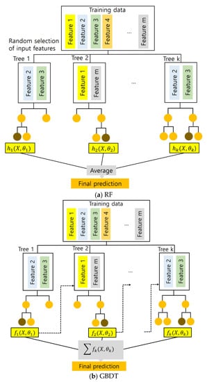
Figure 1.
Schematics of the random forest (RF) and gradient boosted decision tree (GBDT) models.
In this study, both RF and GBDT models were used for the TDI estimation of 419 drinking water treatment plants. The Python open-source libraries of Scikit-learn (for RF) and XGBoost (for GBDT) were used for regression model development [55,56]. XGBoost (XGB) is one of the most popular GBDT implementations developed by Chen and Guestrin [45,54]. Scikit-learn is also a popular Python-based ML library developed by Pedregosa et al. [55].
2.3.2. Model Optimization
The hyperparameters of RF and XGB were optimized by a trial and error method with ten-fold cross-validation using the grid search library in Scikit-learn [57]. The models were developed with 23 input variables of 419 water treatment plants, where the ratio of data used for training and testing of the models was 8:2.
2.3.3. Feature Importance (FI) of Input Variables
The relative importance of input variables on RF and XGB model performance was calculated using the feature importance (FI) algorithm in Scikit-learn [57]. The FI in the tree-based model was computed as the total impurity reduction of the model brought by that feature [55,58,59].
2.3.4. Model Evaluation
The model performance was evaluated by three evaluation indexes (Equations (7)–(9)), RMSE, coefficient of determination (R2), and RMSE-observation standard deviation ratio (RSR). RSR ranges from 0 to 1 and approaches 0 when the model shows a good fit with observation. The model is considered to predict the observation when RSR < 0.70 [60,61].
where
: observed values,
: mean of observed values, and
: model predicted value.
3. Results and Discussion
3.1. Characteristics of Input Variables
Total 23 input variables for the development of DI were identified from open-source public statistical data. The characteristics of the input variables are summarized in Table 3. The frequency of warning advisories of natural disasters was calculated at each water treatment plant from the sum of the three variables in Table 3 (i.e., RAIN, SWIND, and TYPHOON). The frequency of warning advisories ranged from 0.017 to 1.29 times/km2 and tended to be higher in areas near the ocean as shown in Figure 2 using ArcGIS pro.
Table 3.
Characteristics of input variables.
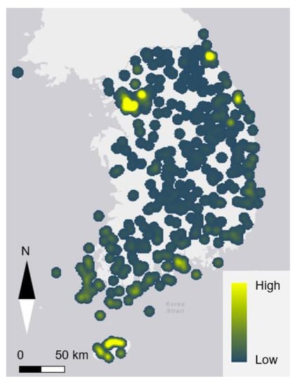
Figure 2.
A spatial distribution of water treatment plants and frequency of natural disasters determined from the disaster warning advisories in Korea.
3.2. Disaster Index (DI) Model Development
3.2.1. PCA Analysis
The weights for each natural disaster index were determined from PCA with 23 input variables (Table 4). The eigenvectors were calculated from PCA and normalized to make the sum of weights of each component to be 1.
Table 4.
PCA analysis for weight of each component.
3.2.2. AHP Analysis
The weights for each disaster type were determined from the AHP analysis using the survey data (CR < 0.2) (Table 5). The response rate of the survey was in the range between 52 and 69% for each item. The weights of each disaster are in the order of typhoons, earthquakes, and heavy rain.
Table 5.
Analytical hierarchy process (AHP) analysis results.
3.2.3. Disaster Index (DI)
The TDI was determined using the following model (Equations (10)–(13)) which were developed from PCA and AHP analysis (Table 4 and Table 5).
where
TDI = 0.481(TI) + 0.198(HI) + 0.321(EI)
TI = 0.275(REt) + 0.265(RIt) + 0.216(URt) − 0.244(RRt)
REt = 0.309(REt1) + 0.345(REt2) + 0.346(REt3),
RIt = 0.143(RIt1) + 0.143(RIt2) + 0.144(RIt3) + 0.052(RIt4) + 0.140(RIt5) + 0.132(RIt6) + 0.136(RIt7) + 0.110(RIt8),
URt = 0.334(URt1) + 0.334(URt2) + 0.332(URt3), and
RRt = 0.248(RRt1) + 0.235(RRt2) + 0.263(RRt3) + 0.254(RRt4).
HI = 0.279(REh) + 0.247(RIh) + 0.221(URh) − 0.253(RRh)
REh = 0.500(REh1) + 0.500(REh2),
RIh = 0.143(RIh1) + 0.143(RIh2) + 0.144(RIh3) + 0.052(RIh4) + 0.140(RIh5) + 0.132(RIh6) + 0.136(RIh7) + 0.110 (RIh8),
URh = 0.334(URh1) + 0.334(URh2) + 0.332(URh3), and
RRh = 0.248(RRh1) + 0.235(RRh2) + 0.263(RRh3) + 0.254(RRh4).
EI = 0.215(REe) + 0.370(RIe) + 0.235(URe) − 0.180(RRe)
REe = 0.333(REe1) + 0.336(REe2) + 0.331(REe3),
RIe = 0.143(RIe1) + 0.143(RIe2) + 0.144(RIe3) + 0.052(RIe4) + 0.140(RIe5) + 0.132(RIe6) + 0.136(RIe7) + 0.110(RIe8),
URe = 0.334(URe1) + 0.334(URe2) + 0.332(URe3), and
RRe = 0.234(RRe1) + 0.056(RRe2) + 0.222(RRe3) + 0.249(RRe4) + 0.239(RRe5).
Using the developed models, TDI values of 419 water treatment plants were determined with the range between −0.526 and 3.813 with an average of 0 and a standard deviation of 0.343. A higher TDI represents a higher potential of effect or damage by a disaster in water treatment systems. The TDI tends to be higher in water treatment plants near metropolitan cities as well as the areas near ocean.
The TDI was developed considering the natural status of Korea. For example, there were only two earthquakes in 2016 and 2017, which were considered to have caused actual damage to water treatment plants in Korea. As the data available for the quantification of damage by earthquakes is minimal, the AHP based on survey data was used for the DI calculation.
Although there were not many cases of damage in water treatment systems from earthquakes, the weight of the earthquake was larger than that of heavy rain. The AHP results represent that, although earthquakes have been rare in Korea, the damage and consequences by an earthquake would not be negligible when it occurs, indicating that a preventive plan against earthquakes should be prepared in advance. In addition, given that most of the facilities already experience heavy rain and are relatively well prepared for these instances, it is expected that the actual damage caused by heavy rain is relatively small compared to other disasters.
3.3. Ensemble Model Simulation
3.3.1. Total Disaster Index (TDI) Prediction using Ensemble Models
Two ensemble ML models, RF and XGB, were used to develop a model to predict TDI. The model performance with the test data set was evaluated by three indices, as summarized in Table 6. The R2 and RSR were 0.8435 and 0.3957 for the RF model and 0.8629 and 0.3703 for the XGB model, respectively.
Table 6.
Summary of model evaluation results.
The observed data and model predictions are compared in Figure 3. The model prediction shows a similar good fit with observations both in the RF and XGB models, while XGB showed a slightly better performance for all three evaluation indexes (Table 6 and Figure 3).
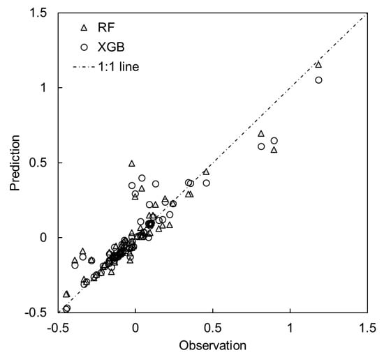
Figure 3.
Comparison of model prediction.
3.3.2. Feature Importance (FI) Analysis
The FI of 23 input variables for both RF and XGB models to predict DI are shown in Figure 4. The FI was different between RF and XGB, while the variables that represent the scale of water treatment plants such as PUMP_EP and Q tend to have a higher effect on model performance for both models. For RF, the sum of FI in the highest nine input variables was more than 80%, while for XGB, the sum of FI in the highest four variables was more than 80% of the total FI for XGB.
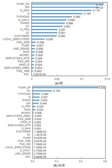
Figure 4.
Feature importance (FI) of (a) RF and (b) XGBoost (XGB).
The performance of the models was compared between RF and XGB using fewer input variables, starting with 1 and adding up to 10 input variables with the order from the highest FI (Figure 5). The RF model showed a tendency to improve the performance of the model as the number of input variables increased from one to ten, and even when using three input variables, the RSR was 0.6954, indicating that the model accurately predicted the observation. XGB shows better performance when using fewer input variables. The RSR is 0.5323 when only three input variables were applied, which reduces to 0.3937 when using ten input variables. The FI analysis shows that several input variables with higher feature importance have a considerable effect on model performance. The analysis results show that both the RF and XGB models show similar performance when using five or more input variables with higher FI. The FI is one of the factors and not an absolute standard considered for model structure. The necessary input variables are not always obtainable from the actual operation and management of water treatment systems. Thus, the practical applicability of the model would be improved as fewer input variables are used. The FI analysis suggests that the model shows acceptable performance if only part of the input variables with the highest FI would increase the practical applicability of the model.
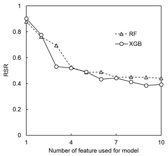
Figure 5.
Model sensitivity to the number of input variables included in a model (RF or XGB).
4. Summary and Conclusions
In this study, a disaster index (DI) for predicting the effect or damage caused by three major natural disasters in Korea (i.e., typhoons, heavy rain, and earthquakes) was newly developed to quantify each natural disaster’s effect on water utilities.
Although the operational data in water utilities provided a good understanding regarding the effect of disasters, the data is usually collected in an individually specified format often site-specific, making it difficult to collect, organize, and analyze the data. In addition, the operational data for water utilities was not easily accessible, limiting the comprehensive development of the DI. Therefore, in this study, the DI of natural disasters in water treatment systems was developed using statistical open-source public data. Two well-defined statistical data analysis methods (i.e., AHP and PCA) were used for the determination of DI.
The open-source public data have greater accessibility and are updated regularly, so the DI can also be updated considering the current status, which is also a significant benefit of using open-source public data. The DI developed in this study may be site-specific at a given location and conditions of water utilities, but the developed framework would be applicable for quantifying the effect of disasters on water treatment systems in other regions with different natural status.
In the second part, two ensemble models (i.e., RF and XGB) were used to develop models to predict TDI. Both RF and XGB showed similar satisfactory performance for prediction of the DI, while the XGB showed a slightly better performance in general. The FI analysis also suggested that the models have sufficient performance for practical use with only several input variables of the highest FI, which can improve the practical applicability of the models.
Quantitative assessment of disaster effects on water treatment systems is essential for better management of the water treatment systems and stable supply of drinking water to the public. However, data related to disaster analysis are often limited and even hardly quantifiable. One of the possible solutions would be to keep collecting data, analyze them statistically, while facilitating frequent discussions from experts experiencing the disasters in their utilities [11,35]. The recent advance of information and communication technologies, such as sensor-based real-time monitoring methods, can provide various continuous monitoring data about the operational condition of water treatment plants and related infrastructure, which can improve the pre- and post-management planning processes [20,22]. However, the quantification and assessment of disasters on water treatment systems are still in an early stage, and the use of field operational data and responses, in particular during disaster events, is currently limited at this time.
This study provided quantified information on the impact of various natural disasters on water treatment systems with open-source public data, which would be useful for creating a plan to reduce damage to water supply systems caused by natural disasters. Further study is warranted to use high-frequency real-time data to improve the model performance and practical applicability.
Author Contributions
Data curation and software, J.P.; conceptualization: J.P., J.-H.P., J.-S.C., J.C.J., K.P., W.H.L. and T.-Y.H.; investigation, J.P., J.-H.P., J.-S.C., J.C.J., K.P., H.C.Y., C.Y.P., W.H.L. and T.-Y.H.; writing-original draft, J.P.; writing—review and editing, J.-H.P., J.-S.C., J.C.J., K.P., H.C.Y., C.Y.P. and T.-Y.H.; project administration, J.P. and J.-H.P.; supervision, J.P. and T.-Y.H.; funding acquisition, J.P. and J.-H.P. All authors have read and agreed to the published version of the manuscript.
Funding
This work was supported by Korea Environment Industry and Technology Institute (KEITI) through Environmental R&D Project on the Disaster Prevention of Environmental Facilities Project, funded by Korea Ministry of Environment (MOE) (2019002870001).
Conflicts of Interest
The authors declare no conflict of interest.
References
- Pan American Health Organization (PAHO). Emergencies and Disasters in Drinking Water Supply and Sewage Systems: Guidelines for Effective Response; PAHO: Washington, DC, USA, 2002; pp. 5–12. [Google Scholar]
- Davis, C.A. Water system service categories, post-earthquake interaction, and restoration strategies. Earthq. Spectra 2014, 30, 1487–1509. [Google Scholar] [CrossRef]
- Matthews, J.C. Disaster resilience of critical water infrastructure systems. J. Struct. Eng. 2016, 142, C6015001. [Google Scholar] [CrossRef]
- World Meteorological Organization (WMO). Atlas of Mortality and Economic Losses from Weather, Climate and Water Extremes (1970–2012); WMO-No. 1123; WMO: Geneva, Switzerland, 2014. [Google Scholar]
- Marzi, S.; Mysiak, J.; Essenfelder, A.H.; Amadio, M.; Giove, S.; Fekete, A. Constructing a comprehensive disaster resilience index: The case of Italy. PLoS ONE 2019, 14, e0221585. [Google Scholar] [CrossRef] [PubMed]
- Beccari, B. A comparative analysis of disaster risk, vulnerability and resilience composite indicators. PLoS Curr. 2016, 8. [Google Scholar] [CrossRef] [PubMed]
- Franc, J.M.; Ingrassia, P.L.; Verde, M.; Colombo, D.; Della Corte, F. A simple graphical method for quantification of disaster management surge capacity using computer simulation and process-control tools. Prehosp. Disast. Med. 2015, 30, 9. [Google Scholar] [CrossRef] [PubMed]
- Cimellaro, G.P.; Reinhorn, A.M.; Bruneau, M. Framework for analytical quantification of disaster resilience. Eng. Struct. 2010, 32, 3639–3649. [Google Scholar] [CrossRef]
- Park, Y.; Han, S.; Choi, S. Development of Disaster Risk Index for Evaluating the Natural Disaster Hazards of High-speed Railroad Facilities. J. Korean Soc. Hazard Mitig. 2019, 19, 1–9. [Google Scholar] [CrossRef][Green Version]
- Rossi, R.J.; Gilmartin, K.J. The Handbook of Social Indicators: Sources, Characteristics, and Analysis; Garland STPM Press: New York, NY, USA, 1980. [Google Scholar]
- Bruce, A.; Brown, C.; Avello, P.; Beane, G.; Bristow, J.; Ellis, L.; Fisher, S.; Freeman, S.G.; Jiménez, A.; Leten, J.; et al. Human dimensions of urban water resilience: Perspectives from Cape Town, Kingston upon Hull, Mexico City and Miami. Water Secur. 2020, 9, 100060. [Google Scholar] [CrossRef]
- Lee, S.; Yoon, H. Development of disaster risk assessment method in river confluence using AHP. J. Korean Soc. Hazard Mitig. 2018, 18, 545–553. [Google Scholar] [CrossRef]
- Zagorecki, A.T.; Johnson, D.E.; Ristvej, J. Data mining and machine learning in the context of disaster and crisis management. Int. J. Emerg. Manag. 2013, 9, 351–365. [Google Scholar] [CrossRef]
- Yu, J.; Zhao, Q.; Chin, C.S. Extracting Typhoon Disaster Information from VGI Based on Machine Learning. J. Mar. Sci. Eng. 2019, 7, 318. [Google Scholar] [CrossRef]
- Chen, J.; Li, Q.; Wang, H.; Deng, M. A machine learning ensemble approach based on random forest and radial basis function neural network for risk evaluation of regional flood disaster: A case study of the Yangtze River Delta, China. Int. J. Environ. Res. Public Health 2020, 17, 49. [Google Scholar] [CrossRef] [PubMed]
- Khouj, M.; Lopez, C.; Sarkaria, S.; Marti, J. Disaster management in real time simulation using machine learning. In Proceedings of the 2011 24th Canadian Conference on Electrical and Computer Engineering (CCECE), Niagara Falls, ON, Canada, 8–11 May 2011; pp. 001507–001510. [Google Scholar]
- Chang, F.J.; Hsu, K.; Chang, L.C. (Eds.) Flood Forecasting Using Machine Learning Methods; MDPI: Basel, Switzerland, 2019. [Google Scholar]
- Chang, F.-J.; Guo, S. Advances in hydrologic forecasts and water resources management. Water 2020, 12, 1819. [Google Scholar] [CrossRef]
- Kao, I.-F.; Zhou, Y.; Chang, L.-C.; Chang, F.-J. Exploring a Long Short-Term Memory based Encoder-Decoder framework for multi-step-ahead flood forecasting. J. Hydrol. 2020, 583, 124631. [Google Scholar] [CrossRef]
- Khan, A.; Gupta, S.; Gupta, S.K. Multi-hazard disaster studies: Monitoring, detection, recovery, and management, based on emerging technologies and optimal techniques. Int. J. Disast. Risk Reduct. 2020, 47, 101642. [Google Scholar] [CrossRef]
- Ofli, F.; Meier, P.; Imran, M.; Castillo, C.; Tuia, D.; Rey, N.; Briant, J.; Millet, P.; Reinhard, F.; Parkan, M. Combining human computing and machine learning to make sense of big (aerial) data for disaster response. Big Data 2016, 4, 47–59. [Google Scholar] [CrossRef]
- Park, J.; Kim, K.T.; Lee, W.H. Recent Advances in Information and Communications Technology (ICT) and Sensor Technology for Monitoring Water Quality. Water 2020, 12, 510. [Google Scholar] [CrossRef]
- Orencio, P.M.; Fujii, M. A localized disaster-resilience index to assess coastal communities based on an analytic hierarchy process (AHP). Int. J. Disast. Risk Reduct. 2013, 3, 62–75. [Google Scholar] [CrossRef]
- Sheykhmousa, M.; Kerle, N.; Kuffer, M.; Ghaffarian, S. Post-disaster recovery assessment with machine learning-derived land cover and land use information. Remote Sens. 2019, 11, 1174. [Google Scholar] [CrossRef]
- Resch, B.; Usländer, F.; Havas, C. Combining machine-learning topic models and spatiotemporal analysis of social media data for disaster footprint and damage assessment. Cartogr. Geogr. Inf. Sci. 2018, 45, 362–376. [Google Scholar] [CrossRef]
- Ragini, J.R.; Anand, P.R.; Bhaskar, V. Big data analytics for disaster response and recovery through sentiment analysis. Int. J. Inf. Manag. 2018, 42, 13–24. [Google Scholar] [CrossRef]
- Zhang, Y.; Zhang, R.; Ma, Q.; Wang, Y.; Wang, Q.; Huang, Z.; Huang, L. A feature selection and multi-model fusion-based approach of predicting air quality. ISA Trans. 2020, 100, 210–220. [Google Scholar] [CrossRef] [PubMed]
- Bi, C.; Fu, B.; Chen, J.; Zhao, Y.; Yang, L.; Duan, Y.; Shi, Y. Machine learning based fast multi-layer liquefaction disaster assessment. World Wide Web 2019, 22, 1935–1950. [Google Scholar] [CrossRef]
- Cao, A.-T.; Tran, T.-T.; Nguyen, T.-H.-X.; Kim, D. Simplified Approach for Seismic Risk Assessment of Cabinet Facility in Nuclear Power Plants Based on Cumulative Absolute Velocity. Nucl. Technol. 2020, 206, 743–757. [Google Scholar] [CrossRef]
- Korea Meteorological Administration Information Portal. Available online: https://data.kma.go.kr (accessed on 28 March 2020).
- Korea Ministry of the Interior and Safety Information Portal. Available online: http://lofin.mois.go.kr/portal/main.do (accessed on 15 April 2020).
- Korea Ministry of Environment (MOE). 2018 Statics of Waterworks; MOE: Sejong, Korea, 2020.
- Korea Ministry of Land, Infrastructure and Transport (MOLIT). Korea Design Standard; MOLIT: Sejong, Korea, 2016; p. 45.
- Razmkhah, H.; Abrishamchi, A.; Torkian, A. Evaluation of spatial and temporal variation in water quality by pattern recognition techniques: A case study on Jajrood River (Tehran, Iran). J. Environ. Manag. 2010, 91, 852–860. [Google Scholar] [CrossRef]
- Tripathi, M.; Singal, S.K. Use of Principal Component Analysis for parameter selection for development of a novel Water Quality Index: A case study of river Ganga India. Ecol. Indic. 2019, 96, 430–436. [Google Scholar] [CrossRef]
- Sahoo, M.M.; Patra, K.; Khatua, K. Inference of water quality index using ANFIA and PCA. Aquat. Procedia 2015, 4, 1099–1106. [Google Scholar] [CrossRef]
- Saaty, T.L. The Analytic Hierarchy Process; Mcgraw Hill: New York, NY, USA, 1980. [Google Scholar]
- Wind, Y.; Saaty, T.L. Marketing applications of the analytic hierarchy process. Manag. Sci. 1980, 26, 641–658. [Google Scholar] [CrossRef]
- Chakraborty, S.; Kumar, R.N. Assessment of groundwater quality at a MSW landfill site using standard and AHP based water quality index: A case study from Ranchi, Jharkhand, India. Environ. Monit. Assess. 2016, 188, 335. [Google Scholar] [CrossRef]
- Saaty, T.L. How to make a decision: The analytic hierarchy process. Eur. J. Oper. Res. 1990, 48, 9–26. [Google Scholar] [CrossRef]
- Saaty, R.W. The analytic hierarchy process—What it is and how it is used. Math. Model. 1987, 9, 161–176. [Google Scholar] [CrossRef]
- Saaty, T.L. Priority setting in complex problems. IEEE Trans. Eng. Manag. 1983, 3, 140–155. [Google Scholar] [CrossRef]
- Uddameri, V.; Silva, A.L.B.; Singaraju, S.; Mohammadi, G.; Hernandez, E.A. Tree-Based Modeling Methods to Predict Nitrate Exceedances in the Ogallala Aquifer in Texas. Water 2020, 12, 1023. [Google Scholar] [CrossRef]
- Shin, Y.; Kim, T.; Hong, S.; Lee, S.; Lee, E.; Hong, S.; Lee, C.; Kim, T.; Park, M.S.; Park, J. Prediction of Chlorophyll-a Concentrations in the Nakdong River Using Machine Learning Methods. Water 2020, 12, 1822. [Google Scholar] [CrossRef]
- Zhang, D.; Qian, L.; Mao, B.; Huang, C.; Huang, B.; Si, Y. A data-driven design for fault detection of wind turbines using random forests and XGboost. IEEE Access 2018, 6, 21020–21031. [Google Scholar] [CrossRef]
- Breiman, L. Random forests. Mach. Learn. 2001, 45, 5–32. [Google Scholar] [CrossRef]
- Genuer, R.; Poggi, J.-M.; Tuleau-Malot, C. Variable selection using random forests. Pattern Recognit. Lett. 2010, 31, 2225–2236. [Google Scholar] [CrossRef]
- Hollister, J.W.; Milstead, W.B.; Kreakie, B.J. Modeling lake trophic state: A random forest approach. Ecosphere 2016, 7, e01321. [Google Scholar] [CrossRef]
- Fernández-Delgado, M.; Cernadas, E.; Barro, S.; Amorim, D. Do we need hundreds of classifiers to solve real world classification problems? J. Mach. Learn. Res. 2014, 15, 3133–3181. [Google Scholar]
- Singh, B.; Sihag, P.; Singh, K. Modelling of impact of water quality on infiltration rate of soil by random forest regression. Model. Earth Syst. Environ. 2017, 3, 999–1004. [Google Scholar] [CrossRef]
- Read, E.K.; Patil, V.P.; Oliver, S.K.; Hetherington, A.L.; Brentrup, J.A.; Zwart, J.A.; Winters, K.M.; Corman, J.R.; Nodine, E.R.; Woolway, R.I. The importance of lake-specific characteristics for water quality across the continental United States. Ecol. Appl. 2015, 25, 943–955. [Google Scholar] [CrossRef] [PubMed]
- Friedman, J.H. Greedy function approximation: A gradient boosting machine. Ann. Stat. 2001, 1189–1232. [Google Scholar] [CrossRef]
- Ke, G.; Meng, Q.; Finley, T.; Wang, T.; Chen, W.; Ma, W.; Ye, Q.; Liu, T.-Y. Lightgbm: A highly efficient gradient boosting decision tree. In Proceedings of the Advances in Neural Information Processing Systems (NIPS 2017), Long Beach, CA, USA, 4–9 December 2017; pp. 3146–3154. [Google Scholar]
- Chen, T.; Guestrin, C. Xgboost: A scalable tree boosting system. In Proceedings of the 22nd ACM SIGKDD International Conference on Knowledge Discovery and Data Mining, San Francisco, CA, USA, 13–17 August 2016; pp. 785–794. [Google Scholar]
- Pedregosa, F.; Varoquaux, G.; Gramfort, A.; Michel, V.; Thirion, B.; Grisel, O.; Blondel, M.; Prettenhofer, P.; Weiss, R.; Dubourg, V. Scikit-learn: Machine learning in Python. J. Mach. Learn. Res. 2011, 12, 2825–2830. [Google Scholar]
- XGBoost. Available online: https://xgboost.readthedocs.io/en/latest/build.html (accessed on 15 February 2020).
- Scikit-Learn. Available online: https://scikit-learn.org/stable/index.html (accessed on 3 January 2020).
- Fabris, F.; Doherty, A.; Palmer, D.; De Magalhães, J.P.; Freitas, A.A. A new approach for interpreting random forest models and its application to the biology of ageing. Bioinformatics 2018, 34, 2449–2456. [Google Scholar] [CrossRef]
- Grömping, U. Variable importance assessment in regression: Linear regression versus random forest. Am. Stat. 2009, 63, 308–319. [Google Scholar] [CrossRef]
- Moriasi, D.N.; Arnold, J.G.; Van Liew, M.W.; Bingner, R.L.; Harmel, R.D.; Veith, T.L. Model evaluation guidelines for systematic quantification of accuracy in watershed simulations. Trans. ASABE 2007, 50, 885–900. [Google Scholar] [CrossRef]
- Bennett, N.D.; Croke, B.F.; Guariso, G.; Guillaume, J.H.; Hamilton, S.H.; Jakeman, A.J.; Marsili-Libelli, S.; Newham, L.T.; Norton, J.P.; Perrin, C. Characterising performance of environmental models. Environ. Model. Softw. 2013, 40, 1–20. [Google Scholar] [CrossRef]


Publisher’s Note: MDPI stays neutral with regard to jurisdictional claims in published maps and institutional affiliations. |
© 2020 by the authors. Licensee MDPI, Basel, Switzerland. This article is an open access article distributed under the terms and conditions of the Creative Commons Attribution (CC BY) license (http://creativecommons.org/licenses/by/4.0/).