Abstract
Joint probability methods for characterizing storm surge hazards involve the use of a collection of hydrodynamic storm simulations to fit a response surface function describing the relationship between storm surge and storm parameters. However, in areas with a sufficiently low probability of flooding, few storms in the simulated storm suite may produce surge, resulting in a paucity of information for training the response surface fit. Previous approaches have replaced surge elevations for non-wetting storms with a constant value or truncated them from the response surface fitting procedure altogether. The former induces bias in predicted estimates of surge from wetting storms, and the latter can cause the model to be non-identifiable. This study compares these approaches and improves upon current methodology by introducing the concept of “pseudo-surge,” with the intent to describe how close a storm comes to producing surge at a given location. Optimal pseudo-surge values are those which produce the greatest improvement to storm surge predictions when they are used to train a response surface. We identify these values for a storm suite used to characterize surge hazard in coastal Louisiana and compare their performance to the two other methods for adjusting training data. Pseudo-surge shows potential for improving hazard characterization, particularly at locations where less than half of training storms produce surge. We also find that the three methods show only small differences in locations where more than half of training storms wet.
1. Introduction
The state of Louisiana and its surrounding coastline have repeatedly been victims of intense tropical storms causing severe damage. In an effort to assess and reduce flood risk, the Louisiana Coastal Protection and Restoration Authority (CPRA) has developed the state’s Comprehensive Master Plan for a Sustainable Coast (CMP), a $50 billion-dollar portfolio of 124 restoration, structural and non-structural projects to be implemented over the next 50 years to mitigate the effects of storm hazards and reduce land loss [1]. To make informed decisions concerning the CMP project portfolio, CPRA commissioned the development of the Coastal Louisiana Risk Assessment (CLARA) model to assess risk due to storm hazards for current, and many possible future, climate conditions [2,3,4].
A key component of the risk assessment calculation is hazard characterization—in this case, an estimate of the annual exceedance probability function (AEPF) for storm surge-based flood depths, commonly referred to as the flood depth exceedance curve. The AEPF returns the probability that a specified flood depth is met or exceeded in a given year. Joint probability methods for estimating flood depth exceedance curves use a collection of hydrodynamic storm simulations to train a response surface model describing the functional relationship between peak storm surge and storm parameters like central pressure deficit and the radius of maximum wind speed [5,6,7,8]. This response surface function is used to predict peak surge resulting from a range of storms, spanning the space of plausible storm parameters, and to then combine the results with simulation data in the final estimation of flood depth exceedances. (In this paper, we focus on characterization of the hazard posed by peak surge levels and ignore other considerations, such as the duration of a flood event or differences in consequences associated with salt- versus freshwater flooding. We also ignore wave behavior, such that “flood depths” refer here to the difference between peak surge elevation and topographic elevation.)
However, in areas with a sufficiently low probability of flooding, few storms in the simulated storm suite may produce surge, with some locations remaining dry in nearly all simulated events. From here on, such a storm which produces no surge at a given location will be described as “non-wetting.” Analysts could treat these zero-depth, non-wetting storms as either truncated or censored data when fitting a response surface. If non-wetting storms are truncated, i.e., removed from the response surface training set, then in some instances, it may be impossible to identify a unique response surface model because the number of covariates exceeds the number of wetting storms. Even if a unique model can be identified, removing non-wetting storms may result in a small-sample problem with correspondingly low confidence in surge predictions. This is further exacerbated by the fact that analysts often restrict the number of simulated storms in order to meet time and budget constraints while balancing bias in flood depth exceedance estimates [9,10,11]. Contemporary methods for decision-making under deep uncertainty and adaptive planning frequently require modeling multiple future time periods under a range of future scenarios, thus constraining the number of storms that can be simulated in any single scenario and time period [12,13].
An alternative approach is to treat surge from non-wetting storms as censored observations with an upper bound equal to the topographic elevation, but this raises the question of how to impute and incorporate these observations into the training set. Past studies by the US Army Corps of Engineers (USACE) assigned a surge elevation equal to three-tenths of the location’s topographic NAVD88 elevation (or a fixed constant value if the location is below zero NAVD88 feet) [14]. This “topographic replacement” approach potentially reduces the predictive performance of the response surface function because it clusters observations by assigning the same surge elevation value despite having different storm parameters.
When truncating or censoring observations, non-wetting storms are thus indistinguishable. In reality, some storms may have been closer to wetting a location than others (i.e., if the storm was slightly more intense or larger). This motivates the concept of an imputed surge, or “pseudo-surge,” value with the intent to quantify how close a storm came to causing surge at a location; such a pseudo-surge would have a negative value relative to the topographic elevation. Ultimately, the goal of exploring the pseudo-surge concept is not to identify how close an individual storm is to causing surge, but to improve predictions of surge from other storms not in a training set of simulated events.
In this paper, we identify the improvement in AEPF estimates from including imputed pseudo-surge values in a response surface training set. We identify optimal pseudo-surge values for a commonly used suite of storms impacting coastal Louisiana [14,15,16]. We then compare the performance of the pseudo-surge values to that produced by currently-used methods for truncating or censoring data, with respect to the predictive accuracy in out-of-sample storms and estimates of flood depth exceedance return periods. Our results demonstrate the potential efficacy of a pseudo-surge implementation and generate a dataset which can be used to measure the performance of candidate null surge replacement rules for use within the Louisiana coastal area. A similar method could be applied to flood risk studies in other coastal regions that experience the same issue with hydrodynamic simulation outputs. We recommend determining optimal pseudo-surge values within the context of a specific geography and storm suite, then using them to develop a rule of thumb to estimate near-optimal pseudo-surge values for non-wetting storms.
For the state of Louisiana, we find that the optimal pseudo-surge values reduce flood depth exceedance estimate bias in regions where fewer than 50% of simulated storms return defined surge. We also demonstrate that simply truncating non-wetting storms from the response surface training set is generally better than following the elevation-based replacement approach utilized by USACE. Because we are unaware of other studies comparing the performance of truncating non-wetting storms to the use of a topographic replacement method, this represents another contribution of the work to our understanding of coastal flood risk.
2. Methods
2.1. Experimental Design
The diagram in Figure 1 illustrates the general model workflow used to generate estimates of the annual exceedance probability function. This study uses climatological conditions, coastal topography and bathymetry, representing coastal Louisiana in the year 2015, to define the state of the world hereafter referred to as “current conditions” [16,17,18]. The hydrodynamic storm simulations are the same coupled ADCIRC+SWAN runs used for estimating risk under current conditions in Louisiana’s 2017 Comprehensive Master Plan for a Sustainable Coast [1]. The white boxes are tasks which are implemented in the CLARA model, and the black box is the task which is the focus of this study.
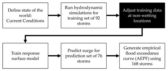
Figure 1.
Workflow for estimating flood depth annual exceedance probability functions using a response surface trained on data adjusted for non-wetting.
ADCIRC+SWAN model simulations are available for the reference set of 168 storms used in the 2017 Coastal Master Plan. These simulation outputs are used as the “gold standard” values for comparison against the results of the response surface model. Figure 2 depicts this more compact workflow. Note that no response surface is implemented in this case because hydrodynamic simulations are available for every storm used to generate the AEPF.
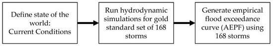
Figure 2.
Workflow for estimating flood depth annual exceedance probability functions from the reference set of 168 storms.
We use a pointwise non-linear optimization to identify the optimal pseudo-surge values that maximally improve predictions of surge from the 76 storms in the prediction set; by “pointwise,” we mean that the algorithm is applied independently at each grid point. We calculate pseudo-surge values for non-wetting storms in the 92-storm simulation set, train a response surface function using the surge and pseudo-surge data, predict surge for storms in the 76-storm prediction set, and then generate a new empirical flood exceedance curve using the combined 168 storms. Mathematical details of the optimization approach used to generate pseudo-surge values are detailed in Appendix A, and the CLARA model’s response surface is described in the next section. The storm parameters at landfall are defined in Table 1 with the values for the 168 storms provided in Table A2.

Table 1.
Covariates of the Coastal Louisiana Risk Assessment (CLARA) model’s surge response surface.
We compare the accuracy of predicted surge elevations from individual storms, and the flood depth AEPF, that result from training the response surface on three different training datasets. The first uses the USACE approach of adopting a censored surge elevation value for non-wetting storms that is based on the topographic elevation. The second removes non-wetting observations from the training data entirely, consistent with CLARA methods. Finally, the third substitutes the optimal pseudo-surge values wherever non-wetting occurs. Given their policy relevance, we focus on the 100 and 500 year return periods from the AEPF (i.e., flood depths with a 1-in-100 or 1-in-500 chance of occurring or being exceeded in a given year).
When assessing accuracy in predicted surge from individual storms, we wish to acknowledge the substantial difference between observing non-wetting and experiencing even a small amount of flooding. Even though the “true” surge value is unobserved and censored in the non-wetting case, we adjust the traditional root mean squared error (RMSE) statistic to include cases where one of the surge or predicted surge values are below the topographic elevation. As such, we calculate for each point and storm , a squared error term as follows, where represents the true surge elevation from the hydrodynamic simulation, the predicted surge elevation, and the topographic elevation. In cases where the true surge and predicted surge are both below the topographic elevation, no error is assigned (given that both are, in effect, non-wetting).
Once the error is defined for each storm in the storm suite , the adjusted RMSE at point is calculated as
2.2. Technical Context
A brief discussion of the technical context is necessary before further detailing methods. In this analysis, we consistently utilize the response surface methodology and grid points developed by the Coastal Louisiana Risk Assessment (CLARA) model. CLARA was developed to support Louisiana’s coastal master planning process [2,4]; its current version generates estimates of risk using a hazard–vulnerability–consequence framework on a variable-resolution grid of 113,691 grid points spanning coastal Louisiana, east Texas, and Mississippi [16]. We restrict our study to points located within Louisiana that are not enclosed by a ringed structural protection system, shown in Figure 3.
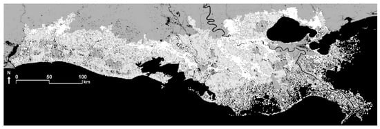
Figure 3.
The CLARA model domain and variable-resolution grid.
Using the coupled ADCIRC+SWAN models, 92 storms from a synthetic storm set are simulated making landfall on the coast, returning peak surge elevation and significant wave heights for each storm at each CLARA grid point in the study region. These data are then used to train a response surface function using the covariates in Table 1 and a nested hierarchy of regression methods.
Full details of the CLARA response surface procedure are found in Fischbach et al. [16], but briefly, the model hierarchy is as follows, in order of priority.
- (1)
- Conditionally Parametric Locally Weighted Regression (CPARLWR) [19] with full model specification (the local weighting of observations from nearby grid points is limited to points within regions of similar hydrology, i.e., the same watershed):
- (2)
- Point-level ordinary least squares regression with full model specification.
- (3)
- Point-level ordinary least squares regression with a reduced-form model:
- (4)
- Point- and track-level ordinary least squares regression with reduced-form model:
- (5)
- Step function assigning equal surge elevation and wave heights to any synthetic storms more extreme than wetting storms from the simulation set.
The hierarchy of response surface specifications outlined here is unique to the CLARA model, which potentially limits the generalizability of our results. However, we note that the reduced-form model originates in the broader literature on joint probability modeling of storm surge [6,20], so many other studies and models have utilized identical or very similar model specifications. We expect that pseudo-surge or the truncation approach could produce greater improvements, relative to the topographic replacement, in other models using simpler structural forms. Because of CPARLWR’s similarity to universal kriging (i.e., kriging with covariates or regression-kriging), we expect that results may also be similar for models using that approach; Selby and Kockelman (2013) and Meng (2014) provide more detailed comparisons between kriging and geographically weighted regression methods [21,22].
Because the CLARA model’s default methodology removes non-wetting storms from the training data, it is possible that the full CPARLWR model may not be identifiable in cases with few wetting storms. As wetting storms become more and more sparse, the procedure reverts to regression techniques which require fewer covariates, thus requiring fewer wetting storms to identify. The method with the highest priority employs local weighting, which assumes that grid points near each other experience similar levels of surge, leveraging their observations to increase the effective sample size; a bandwidth parameter, that defines how quickly weights decay with distance, is tuned to optimize predictive accuracy within each watershed. When the locally-weighted regression model fails to identify, subsequent models attempt to fit a linear function to surge data independently at each grid point.
The sparsity of data is a result of the nature of the hydrodynamic simulation outputs. For grid points with a sufficiently low probability of flooding, most synthetic storms will return an undefined surge value which indicates that no wetting occurs at that location. Figure 4 shows the extent of this behavior at each grid point using the percentage of the 92 simulated training storms for which the hydrodynamic simulation returned a defined value. Since the focus of our analysis is on null-value storms and their potential replacements, we exclude points that wet in all 92 storms, as well as points that do not wet in any of the 92 storms.
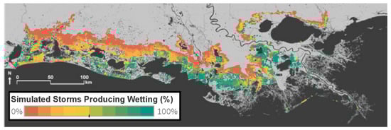
Figure 4.
Percentage of storms in the 92-storm training set that produce wetting, by location (grid points with 0% or 100% wetting are omitted).
Truncating storm data for undefined storms can affect the quality and ability to fit a high-priority response surface regression method. Figure 5 shows the model used in each grid point where at least one storm in the 92-storm suite is non-wetting. From this figure, we can verify our intuition that simpler parameterizations get employed further inland where fewer storms wet.
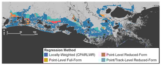
Figure 5.
Response surface model utilized by CLARA’s default methodology under current conditions (omitted: grid points where all or no training storms produce surge).
Using the topographic elevation-based replacement or the imputed pseudo-surge values allows us to avoid dropping any observations from the dataset. The elevation-based approach replaces non-wetting storms with an identical value regardless of the storm parameters, so there is still a small possibility that the resulting data would have insufficient variation to identify the full-form model. However, the pseudo-surge approach produces variable surge elevation values, such that the full-form locally weighted model should always be employed.
2.3. Training and Prediction Storms
The 92 storm simulations used as the training set and 168 storms used to form the AEPF curves represent the training and prediction sets used to estimate risk under the current conditions landscape in Louisiana’s 2017 Coastal Master Plan. They were originally selected from a suite of 446 storm simulations developed by the U.S Army Corps of Engineers for previous flood risk studies in coastal Louisiana [14,15]. Full details of the procedure for storm set reduction are provided in Fischbach et al. (2016) [10], and the storm surge and wave outputs for all 446 storms are publicly available upon request to the Louisiana Coastal Protection and Restoration Authority. The storm parameters at landfall of the 168 storms from this analysis are provided in Appendix B.
Sixteen different subsets of the 446 storms were evaluated, with each subset ranging from 40 to 154 storms. The 92-storm set was selected for modeling risk under the current conditions landscape on the basis of its balance of predictive accuracy (when compared to AEPF curves derived from all 446 storms) and the total number of ADCIRC+SWAN simulations required. Analysis indicated that further reducing the sample of storms tended to increase bias relative to the 446-storm suite.
The set consists of 6 storms with central pressure ranging from 900 to 975 mb on ten different storm tracks that approach landfall at the mean heading observed from historic storms. Four storms (two each with of 960 and 975 mb), with headings 45 degrees in either direction from the mean angle, were added to four tracks in the eastern half of the state. The additional 76 storms comprising the 168-storm prediction set are run through CLARA, but not ADCIRC+SWAN, using surge and wave characteristics predicted by CLARA’s response surface modeling hierarchy.
The 92- and 168-storm sets used in this analysis were purposively sampled to be a minimal high-performing storm corpus. Consequently, we expect that omitting additional storms from the training set could introduce substantial bias to AEP estimates, particularly in the regions (shown in Figure 5) where the track-by-track reduced-form model is utilized. As such, we do not perform k-fold or leave-one-out cross-validation in this analysis, despite its ordinary importance in evaluating the robustness of prediction methods against the uncertainty associated with randomness of observed training data. This also means that improvements seen in this analysis may be understated, because the training sample was purposively selected to emulate results from a larger storm suite populated with a larger number of wetting storms.
3. Results
Consistent with intuition, we find that the differences between approaches varies substantially according to the number of non-wetting storms observed at a given location. As such, we group the CLARA grid points by their observation density, i.e., the percentage of storms in the training set that produce wetting. Table 2 bins the observation density into deciles and reports the number of CLARA grid points in each bin. These bins partition the grid points depicted in Figure 4. By comparison, the study domain contains 18,213 grid points in which all 92 training storms wet.
Table 2.
Count of CLARA grid points, binned by the percentage of hydrodynamic storm simulations in the training set which returned a defined surge value.
First, we show in Figure 6 the proportion of storms which the response surface correctly classifies as being either wetting or non-wetting when trained using a dataset adjusted by each of the three methods. Replacing non-wetting surge values with a constant value determined by the topographic elevation is the worst performer across the board, correctly classifying storm wetting status substantially less frequently at locations where 10–50 percent of training storms wet. The CLARA method of truncating non-wetting storms from the data and the pseudo-surge imputation method produce generally similar results; the former performs better when more than 40 percent of training storms wet, while the latter does a better job when fewer storms produce surge. This suggests that once a sufficient number of wetting storms can be used to train the response surface, replacing non-wetting storms with negative pseudo-surge values can actually be counter-productive. This finding is consistent with our results for the predictive accuracy of both surge from individual storms and statistical exceedances, as shown in the ensuing figures.
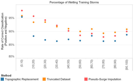
Figure 6.
Wetting classification rate by method, stratified by the percentage of wetting training storms.
Next, we examine the predictive accuracy of each method in estimating the surge produced by the 168 storms in the current conditions storm suite. Figure 7 shows this, grouping grid points by the decile bins described above. We find that the topographic elevation-based replacement method used by USACE generally yields a higher adjusted RMSE than the other two approaches, and the difference in performance is most clear at grid points with a smaller percentage of wetting storms, i.e., 40 or 50 percent or less. This makes intuitive sense, given that the method would introduce a large number of storm surge elevations clustered on the same value; because multiple non-wetting storms of varying severity are assigned the exact same surge elevation, this consequently biases the estimated marginal effects of storm parameters on surge downwards and increases prediction error.
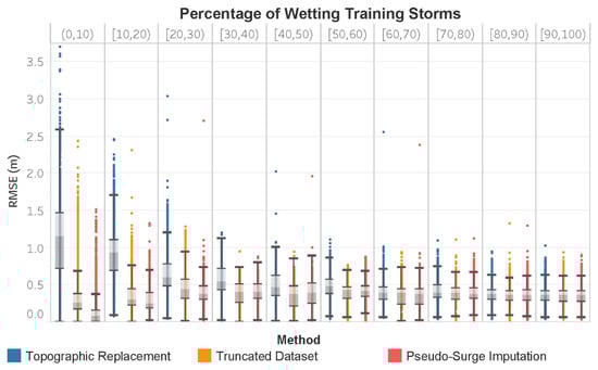
Figure 7.
Root mean square error of predicted surge elevations for individual storms, averaged by grid point and grouped according to the proportion of wetting training storms.
The truncation approach used by CLARA performs similarly to the pseudo-surge method when 30 percent or more training storms wet. For points with fewer wetting storms, utilizing pseudo-surge values produces an improvement. The difference between these two approaches is most stark when less than 10 percent of the training storms wet; this can be attributed to the fact that removing non-wetting storms from the training data results in a very small sample with which to estimate marginal effects with respect to multiple storm and grid point characteristics. This introduces more outliers to the predictions and also causes the model to fall back on the simpler, less accurate response surface models in CLARA’s hierarchy.
Once surge has been predicted for all of the individual storms, the results can be weighted according to the relative likelihood of observing each storm’s characteristics, producing the AEPF. Figure 8 and Figure 9 show the adjusted RMSE values by grid point for the 100 and 500 year flood depth exceedances (based only on storm surge, excluding waves), again grouped by the decile bins of how many training storms wet each point. The inter-quartile range of RMSE for 100 year flood depths is slightly larger for the topographic replacement method when wetting storms are few in number, but the overall differences between approaches are much smaller than for individual storms. Again, however, this is consistent with intuition: locations with very few wetting storms are much more likely to be outside of the 100 year floodplain, such that all three methods would correctly identify the 100 year flood depths as being 0 m.
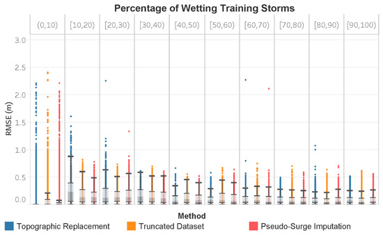
Figure 8.
Root mean squared error of 100 year flood depths by data processing method, compared to the 168-storm reference set and grouped by proportion of wetting training storms.
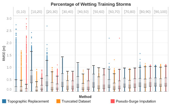
Figure 9.
Root mean squared error of 500 year flood depths by data processing method, compared to the 168-storm reference set and grouped by proportion of wetting training storms.
The relatively poor performance of the topographic replacement method is more apparent at the 500 year return period shown in Figure 9. Differences are quite pronounced for grid points with 10–50 percent wetting storms in the training set. It may be that points with less than 10 percent wetting storms are also near the envelope of the 500 year floodplain, such that the median and 75th percentile values shown in the box-and-whisker plots correspond to points with zero or very small 500 year flood depths. The much larger RMSE values for outliers in the (0,10) bin can be explained by observing that misclassifying small numbers of non-wetting storms as wetting can, at the 500 year return period, mean the difference between zero and sometimes substantial non-zero flood depth exceedances.
The differences between methods shown in the previous figures depend on the observation density of wetting storms in the training data. Consequently, we stratify the adjusted RMSE values in Figure 10 to show how the accuracy of estimated flood depth exceedances varies over a range of return periods. The top pane shows the RMSE for points where less than half of the training storms wet, and the bottom pane points where at least half of them wet. In both cases, we show results from the 10 year to 2000 year return periods and only include points where the flood depth exceedances estimated by the reference set of all 168 storms are non-zero.
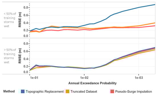
Figure 10.
Adjusted root mean squared error (RMSE) for flood depth exceedances, with return periods ranging from 10 to 2000 years, calculated over all CLARA grid points with non-zero exceedances estimated using the reference dataset.
We see that the differences between methods are very small when the majority of training storms wet (bottom pane). Intuitively, the response surface predictions are less sensitive to adjustments to the training data when fewer adjustments are needed, such that all three methods produce similar results. Estimates of the 10 to 200 year exceedances have an RMSE of approximately 0.2 m at such points, with greater error in estimates of the 250 to 2000 year exceedances.
However, at points where less than half of the training storms produce surge (top pane), using the truncated dataset still performs reasonably well across all return periods, with a maximum difference of 0.1 m at the 25 year return period compared to the pseudo-surge method (adjusted RMSEs of 0.31 m and 0.21 m, respectively). The topographic replacement method performs similarly to truncating the dataset for larger AEPs, but its accuracy diminishes rapidly for less frequent events (i.e., the 100 to 2000 year return periods).
4. Discussion
We have demonstrated that optimal pseudo-surge values have the potential to increase the predictive accuracy of storm surge response surface models, particularly in locations where less than half of training storms wet. By comparing this approach to the topographic replacement and truncation methods, we have shown the extent to which topographic elevation-based replacements perform worse, particularly where wetting training storms are sparse or when estimating more extreme exceedances beyond the 100 year return period. In locations where more than half of training storms wet, truncating non-wetting storms from the training data does not seem to impose much of a sacrifice in predictive accuracy.
The pseudo-surge approach enables the use of larger sample sizes in regression-based models, compared to truncating the data, without the disadvantage of making all non-wetting storms indistinguishable in the surge/wave output space, as in the topographic replacement method. However, we note that this is only one potential solution for the non-wetting storm problem, and its usefulness is primarily limited to approaches that are not capable of representing non-continuous data. Neural networks and kernel-based methods such as support vector machines have been used in recent years for storm surge prediction and could feasibly be used to address the issues of storm set reduction and non-wetting storms; Mosavi et al. (2018) provides a recent review of such approaches [23]. Even within a regression-based framework, a two-stage process inspired by zero-inflated models could also conceivably improve estimates of AEP functions. However, parametric regression-based models are still very common in practice, so truncation or pseudo-surge imputation could provide benefits as an easy-to-implement modification to existing code bases, or to improve past studies through straightforward reanalysis of existing simulation data.
We should emphasize that imputing pseudo-surge values is not currently an operational modeling approach, because it relies on having actual hydrodynamic simulation data to optimize against. In practice, analysts should instead use whatever simulation data are available when training a response surface. However, we believe that the analysis presented in this paper is useful to illustrate the potential improvements in risk assessment if an oracle could replace non-wetting surge values with pseudo-surge values below the topographic elevation in a manner that optimally improves predictive accuracy. This is somewhat similar to calculating the expected value of perfect information. We have shown that the pseudo-surge concept has potential value in locations where less than half of the training storms wet. We also observe that in some other locations, it is actually better to truncate the dataset and train a response surface on a smaller sample than to replace the non-wetting values with any value at all. Doing so may result in better classification of individual storms as either wetting or non-wetting. Comparing the topographic replacement and data truncation approaches to the pseudo-surge imputation method also provides a helpful benchmark for how accurate exceedance estimates could be when using a response surface to predict surge from out-of-sample storms.
5. Conclusions
This paper (i) introduces the pseudo-surge concept and (ii) suggests that truncation of non-wetting storms from training sets is generally preferable to replacement of non-wetting surge codes with constant topographic elevation values. However, we note a limitation of this work, which is that the approaches compared here have only been implemented with the particular response surface specification used by the CLARA model. We would like to further investigate the value of both the pseudo-surge and truncation approaches under a variety of other surrogate model specifications or in conjunction with machine learning techniques.
Accordingly, we propose that a suitable direction for future research would be to identify a statistical approach for estimating near-optimal pseudo-surge values. At locations with a small number of wetting training storms, one might insert a value for the non-wetting storm by referencing a general rule that estimates pseudo-surge as a function of the topographic elevation of the non-wet location, distance between the non-wetting location to the nearest wetting location, and/or other physical characteristics of the storm and landscape. This paper advances a key step in the development of such a rule, which is to first find optimal pseudo-surge values that best minimize the error of the response surface predictions.
Additionally, we note that the similarity in results between the pseudo-surge method and simply truncating the dataset may be attributable to the CLARA model’s hierarchy of response surface models. We are not aware of any systematic reviews of how other coastal flood risk models or studies generally handle the possibility of non-identifiable response surface models due to non-wetting. However, our comparison with the USACE practice, using a constant replacement value related to the topographic elevation, suggests that simple removal of non-wetting values from the data may lead to improved performance when employed in combination with a hierarchical response surface model equipped to handle smaller sample sizes. Future research should also consider the extent to which the results presented here are generalizable to other models and geographic locations.
Author Contributions
Corresponding author D.R.J. developed the CLARA model, the concept of pseudo-surge, and final versions of visualizations. Author M.P.S. derived optimal pseudo-surge values, modified the CLARA model to implement the alternative training datasets, conducted the analysis of results, and developed the metrics used to evaluate model performance. Both authors collaborated on the writing and organization of the manuscript. All authors have read and agreed to the published version of the manuscript.
Funding
Original development of the CLARA model was funded by the Louisiana Coastal Protection and Restoration Authority under Master Service Agreements in support of Louisiana’s 2012 and 2017 Coastal Master Plans. Matthew Shisler’s contributions to this analysis were funded by the U.S. Air Force and made possible by the Purdue Military Research Initiative.
Acknowledgments
The authors thank Hugh Roberts and Zach Cobell for producing the ADCIRC+SWAN hydrodynamic simulations used to inform the training datasets, as well as the Master Plan’s Modeling and Development Teams.
Conflicts of Interest
The authors declare no conflict of interest. The funders had no role in the design of the study; in the collection, analyses, or interpretation of data; in the writing of the manuscript, or in the decision to publish the results.
Appendix A. Identifying the Optimal Pseudo-Surge Values
A mathematical description of the “optimal pseudo-surge” problem now follows. Let be the set of all locations and be the set of all storms. For notational convenience, define Consider the function to be the true unknowable storm surge elevation function. Note that there exist some storms which do not generate surge at some locations, such that is undefined. Often in this discussion we will refer to a partition of the domain into two sets—one of which refers to situations where surge is defined and another which refers to situations where surge is undefined. Let and .
Consider a simulation oracle which grants us the ability to observe when it exists. Define a predictive storm surge function, parameterized by a real vector and constrained to be a linear function of the form
where has dimension , requiring us to estimate coefficients. Our goal is to identify a “best-fit” vector of regression coefficients that minimizes the difference between and .
In practice, it is not possible to know the value of or even whether it exists for all , as this would require an infinite number of simulations. Instead, a discrete number of carefully chosen simulations is used to construct a “simulation” set where . Note that there exists such that is undefined. Then partition in the same manner as letting and . The regression error is defined to be
If non-wetting storms are truncated, then the best fit vector is obtained by minimizing
This minimization includes only wetting storms, , and cannot include non-wetting storms, .
Once is obtained, the function is used to make predictions of for a discrete number of that form a “prediction” set . Note that the simulation prediction sets are disjoint (), and that they do not partition the set of all location–storm pairs (). It is possible that there exists such that is undefined, but this is unknown because there are no simulations for . Nonetheless, partition in the same manner as and , letting and . Note that when , , and are partitioned, we only partition the storm set and not the location set; the same locations are used for evaluating in all cases. Table A1 summarizes each set and the relationships between them.
Table A1.
Location–storm set definitions.
Table A1.
Location–storm set definitions.
| Set | Description | Relationships |
|---|---|---|
| All locations | - | |
| All storms | - | |
| All location–storm pairs | ||
| Location–storm pairs where the storm is wetting | ||
| Location–storm pairs where the storm is non-wetting | , , | |
| Simulation set location–storm pairs | ||
| Wetting simulation set location–storm pairs | ||
| Non-wetting simulation set location–storm pairs | , , | |
| Prediction set location–storm pairs | , , | |
| Wetting prediction set location–storm pairs | ||
| Non-wetting prediction set location–storm pairs | , , |
In a testing situation where is known for , we define the prediction error to be
where is the topographic elevation at location , is a vector of regression coefficients, and is an indicator function for when the function incorrectly predicts surge to exist for . The prediction error is a combination of estimated error for wetting storms and non-wetting storms in the prediction set. A measure of the total error is the sum of the regression error and the prediction error
Note that the first summation is over all wetting storms in the simulation and prediction sets, while the second summation is over only non-wetting storms in the prediction set.
A natural way to improve flood depth exceedance probability function estimates is to improve the similarity between the true storm surge function and the predictive storm surge function . In the current response surface methodology, is obtained using wetting storms in the simulation set, for , which fails to take advantage of information from non-wetting storms in the simulation set, . The fact that is undefined for is itself valuable information.
At this point, we introduce the concept of “pseudo-surge” to be used for non-wetting storms in the simulation set, , with the requirement that a pseudo-surge value remain lower than the topographic elevation, . Let these values be arranged in a vector, . The intent is to identify pseudo-surge values which will improve the similarity between and through the regression coefficients—that is, to use both and for to determine the optimal regression coefficients
where refers to optimal regression coefficients found using pseudo-surge values. We will use the “~” to denote instances where regression coefficients are generated under a pseudo-surge implementation.
In efforts to develop and evaluate a pseudo-surge selection rule for use in other future states of the world, we wish to find the pseudo-surge values which minimize the total error, . For notational convenience, consider the regression coefficients to be a function of the pseudo-surge vector , and the regression and prediction errors to be functions of . Then the optimal pseudo-surge values solve the problem
This formulation maintains the fact that the regression coefficients of the response surface function are to be determined using data from the simulation set only. To solve this problem, we use a non-linear optimization formulation applied to the CLARA grid point as the geospatial unit of analysis.
Pointwise Selection of Optimal Pseudo-surge
The pointwise selection of optimal pseudo-surge values considers each CLARA grid point independently, corresponding to regression method 2 of the response surface hierarchy, point-by-point full-form linear regression.
At this stage, it is more convenient to switch to vector notation when discussing a non-linear optimization approach. The set definitions from Table A1 still hold. Instead of referring to a surge value as a function of a location–storm ordered pair, let represent a vector of storm surge values. Subscript notation is used when referring to surge values for all or some subset of . For example, and refer to surge values for and respectively. Further, let be the covariate matrix for the simulation set of storm data and be the covariate matrix for the prediction set of storm data. A row in these matrices contains the full-form linear regression covariate information for one simulated surge observation. For example, the vector is the vector of surge values which are defined for and is a matrix of corresponding covariate data. Given , surge estimates are then The following discussion applies to a single location (i.e., CLARA grid point) , but we do not use a location subscript to avoid making the necessary notation any more complicated.
The error associated with fitting a linear regression to data and is given as
The analytic solution for the vector which minimizes is
The goal is to construct a vector of optimal coefficients, , using the entirety of the simulation set data and . Let and let be a vector of decision variables representing an ideal form of where all entries are defined either with an original surge value or with a pseudo-surge value. The analytic solution for the vector is
The regression error is then
The prediction error is
where is an indicator vector with elements equal to when the corresponding surge estimate is above the topographic elevation and otherwise. Note that regression error is still measured for wetting simulation set storms only. The first term of the prediction error is for wetting storms, while the second term measures error for non-wetting storms. The vectors and and matrices and are concatenated to produce and , respectively. The total error in vector notation is given as
Choosing pseudo-surge values for entries of is then equivalent to solving the problem
where and are the rows of which correspond to the central pressure and radius of maximum windspeed covariates.
The first two constraints indicate that for all non-wetting storms (undefined surge), the pseudo-surge value must be less than the topographic elevation, , and that for all wetting storms (defined surge), the corresponding decision variable must equal the original surge value from . The last two constraints require that the estimated surge must have a negative relationship with central pressure and a positive relationship with the radius of maximum windspeed.
Solving this minimization problem requires the implementation of a non-linear optimization algorithm such as sequential quadratic programming (SQP) or the interior-point method [24]. The regression and prediction error term in this non-linear optimization invokes the convex vector norm. The error for non-wetting storms in the prediction set, , is also convex, since the argument of the norm is a vector with arguments that are non-negative. As a sum of convex functions, the objective function is convex. For this analysis, we utilize SQP to identify the optimal pseudo-surge values.
This is considered a one-sided loss and is not necessarily foreign to the field of classification problems. Other loss functions for classification exist, such as indicator, logistic, and hinge loss [25]. However, one benefit of a one-sided squared error loss is that it severely penalizes gross misclassification of non-wetting storms. Additionally, all constraints are linear, making the problem amenable to standard non-linear convex optimization algorithms. This is an approach that is independently applied to each CLARA grid point sequentially and therefore can at best produce a point-specific full-form regression model.
Appendix B. Table of Storm Parameters
This table provides the synthetic storm characteristics at landfall of each of the 168 storms included in this study. The parameters are as defined in Table A2. The “training” column indicates whether the storm is one of the 92 included in the training set.
Table A2.
Synthetic storm parameters at landfall.
Table A2.
Synthetic storm parameters at landfall.
| ID | cp | rmax | vf | x | Training | |
|---|---|---|---|---|---|---|
| 1 | 960 | 11 | 11 | 0 | −91.211 | Yes |
| 2 | 960 | 21 | 11 | 0 | −91.211 | No |
| 3 | 960 | 35.6 | 11 | 0 | −91.211 | Yes |
| 4 | 930 | 8 | 11 | 0 | −91.211 | No |
| 5 | 930 | 17.7 | 11 | 0 | −91.211 | Yes |
| 6 | 930 | 25.8 | 11 | 0 | −91.211 | No |
| 7 | 900 | 6 | 11 | 0 | −91.211 | Yes |
| 8 | 900 | 14.9 | 11 | 0 | −91.211 | No |
| 9 | 900 | 21.8 | 11 | 0 | −91.211 | Yes |
| 10 | 960 | 11 | 11 | 0 | −90.451 | Yes |
| 11 | 960 | 21 | 11 | 0 | −90.451 | No |
| 12 | 960 | 35.6 | 11 | 0 | −90.451 | Yes |
| 13 | 930 | 8 | 11 | 0 | −90.451 | No |
| 14 | 930 | 17.7 | 11 | 0 | −90.451 | Yes |
| 15 | 930 | 25.8 | 11 | 0 | −90.451 | No |
| 16 | 900 | 6 | 11 | 0 | −90.451 | Yes |
| 17 | 900 | 14.9 | 11 | 0 | −90.451 | No |
| 18 | 900 | 21.8 | 11 | 0 | −90.451 | Yes |
| 19 | 960 | 11 | 11 | 0 | −89.848 | Yes |
| 20 | 960 | 21 | 11 | 0 | −89.848 | No |
| 21 | 960 | 35.6 | 11 | 0 | −89.848 | Yes |
| 22 | 930 | 8 | 11 | 0 | −89.848 | No |
| 23 | 930 | 17.7 | 11 | 0 | −89.848 | Yes |
| 24 | 930 | 25.8 | 11 | 0 | −89.848 | No |
| 25 | 900 | 6 | 11 | 0 | −89.848 | Yes |
| 26 | 900 | 14.9 | 11 | 0 | −89.848 | No |
| 27 | 900 | 21.8 | 11 | 0 | −89.848 | Yes |
| 28 | 960 | 11 | 11 | 0 | −89.276 | Yes |
| 29 | 960 | 21 | 11 | 0 | −89.276 | No |
| 30 | 960 | 35.6 | 11 | 0 | −89.276 | Yes |
| 31 | 930 | 8 | 11 | 0 | −89.276 | No |
| 32 | 930 | 17.7 | 11 | 0 | −89.276 | Yes |
| 33 | 930 | 25.8 | 11 | 0 | −89.276 | No |
| 34 | 900 | 6 | 11 | 0 | −89.276 | Yes |
| 35 | 900 | 14.9 | 11 | 0 | −89.276 | No |
| 36 | 900 | 21.8 | 11 | 0 | −89.276 | Yes |
| 37 | 960 | 11 | 11 | 0 | −88.647 | Yes |
| 38 | 960 | 21 | 11 | 0 | −88.647 | No |
| 39 | 960 | 35.6 | 11 | 0 | −88.647 | Yes |
| 40 | 930 | 8 | 11 | 0 | −88.647 | No |
| 41 | 930 | 17.7 | 11 | 0 | −88.647 | Yes |
| 42 | 930 | 25.8 | 11 | 0 | −88.647 | No |
| 43 | 900 | 6 | 11 | 0 | −88.647 | Yes |
| 44 | 900 | 14.9 | 11 | 0 | −88.647 | No |
| 45 | 900 | 21.8 | 11 | 0 | −88.647 | Yes |
| 46 | 960 | 18.2 | 11 | −45 | −91.368 | Yes |
| 47 | 960 | 24.6 | 11 | −45 | −91.368 | Yes |
| 48 | 900 | 12.5 | 11 | −45 | −91.368 | No |
| 49 | 900 | 18.4 | 11 | −45 | −91.368 | No |
| 50 | 960 | 18.2 | 11 | −45 | −90.724 | Yes |
| 51 | 960 | 24.6 | 11 | −45 | −90.724 | Yes |
| 52 | 900 | 12.5 | 11 | −45 | −90.724 | No |
| 53 | 900 | 18.4 | 11 | −45 | −90.724 | No |
| 54 | 960 | 18.2 | 11 | −45 | −89.921 | Yes |
| 55 | 960 | 24.6 | 11 | −45 | −89.921 | Yes |
| 56 | 900 | 12.5 | 11 | −45 | −89.921 | No |
| 57 | 900 | 18.4 | 11 | −45 | −89.921 | No |
| 58 | 960 | 18.2 | 11 | −45 | −89.105 | Yes |
| 59 | 960 | 24.6 | 11 | −45 | −89.105 | Yes |
| 60 | 900 | 12.5 | 11 | −45 | −89.105 | No |
| 61 | 900 | 18.4 | 11 | −45 | −89.105 | No |
| 66 | 960 | 18.2 | 11 | 45 | −90.994 | Yes |
| 67 | 960 | 24.6 | 11 | 45 | −90.994 | Yes |
| 68 | 900 | 12.5 | 11 | 45 | −90.994 | No |
| 69 | 900 | 18.4 | 11 | 45 | −90.994 | No |
| 70 | 960 | 18.2 | 11 | 45 | −90.214 | Yes |
| 71 | 960 | 24.6 | 11 | 45 | −90.214 | Yes |
| 72 | 900 | 12.5 | 11 | 45 | −90.214 | No |
| 73 | 900 | 18.4 | 11 | 45 | −90.214 | No |
| 74 | 960 | 18.2 | 11 | 45 | −89.638 | Yes |
| 75 | 960 | 24.6 | 11 | 45 | −89.638 | Yes |
| 76 | 900 | 12.5 | 11 | 45 | −89.638 | No |
| 77 | 900 | 18.4 | 11 | 45 | −89.638 | No |
| 78 | 960 | 18.2 | 11 | 45 | −89.047 | Yes |
| 79 | 960 | 24.6 | 11 | 45 | −89.047 | Yes |
| 80 | 900 | 12.5 | 11 | 45 | −89.047 | No |
| 81 | 900 | 18.4 | 11 | 45 | −89.047 | No |
| 201 | 960 | 11 | 11 | 0 | −94.22 | Yes |
| 202 | 960 | 21 | 11 | 0 | −94.22 | No |
| 203 | 960 | 35.6 | 11 | 0 | −94.22 | Yes |
| 204 | 930 | 8 | 11 | 0 | −94.22 | No |
| 205 | 930 | 17.7 | 11 | 0 | −94.22 | Yes |
| 206 | 930 | 25.8 | 11 | 0 | −94.22 | No |
| 207 | 900 | 6 | 11 | 0 | −94.22 | Yes |
| 208 | 900 | 14.9 | 11 | 0 | −94.22 | No |
| 209 | 900 | 21.8 | 11 | 0 | −94.22 | Yes |
| 210 | 960 | 11 | 11 | 0 | −93.558 | Yes |
| 211 | 960 | 21 | 11 | 0 | −93.558 | No |
| 212 | 960 | 35.6 | 11 | 0 | −93.558 | Yes |
| 213 | 930 | 8 | 11 | 0 | −93.558 | No |
| 214 | 930 | 17.7 | 11 | 0 | −93.558 | Yes |
| 215 | 930 | 25.8 | 11 | 0 | −93.558 | No |
| 216 | 900 | 6 | 11 | 0 | −93.558 | Yes |
| 217 | 900 | 14.9 | 11 | 0 | −93.558 | No |
| 218 | 900 | 21.8 | 11 | 0 | −93.558 | Yes |
| 219 | 960 | 11 | 11 | 0 | −92.964 | Yes |
| 220 | 960 | 21 | 11 | 0 | −92.964 | No |
| 221 | 960 | 35.6 | 11 | 0 | −92.964 | Yes |
| 222 | 930 | 8 | 11 | 0 | −92.964 | No |
| 223 | 930 | 17.7 | 11 | 0 | −92.964 | Yes |
| 224 | 930 | 25.8 | 11 | 0 | −92.964 | No |
| 225 | 900 | 6 | 11 | 0 | −92.964 | Yes |
| 226 | 900 | 14.9 | 11 | 0 | −92.964 | No |
| 227 | 900 | 21.8 | 11 | 0 | −92.964 | Yes |
| 228 | 960 | 11 | 11 | 0 | −92.317 | Yes |
| 229 | 960 | 21 | 11 | 0 | −92.317 | No |
| 230 | 960 | 35.6 | 11 | 0 | −92.317 | Yes |
| 231 | 930 | 8 | 11 | 0 | −92.317 | No |
| 232 | 930 | 17.7 | 11 | 0 | −92.317 | Yes |
| 233 | 930 | 25.8 | 11 | 0 | −92.317 | No |
| 234 | 900 | 6 | 11 | 0 | −92.317 | Yes |
| 235 | 900 | 14.9 | 11 | 0 | −92.317 | No |
| 236 | 900 | 21.8 | 11 | 0 | −92.317 | Yes |
| 237 | 960 | 11 | 11 | 0 | −91.654 | Yes |
| 238 | 960 | 21 | 11 | 0 | −91.654 | No |
| 239 | 960 | 35.6 | 11 | 0 | −91.654 | Yes |
| 240 | 930 | 8 | 11 | 0 | −91.654 | No |
| 241 | 930 | 17.7 | 11 | 0 | −91.654 | Yes |
| 242 | 930 | 25.8 | 11 | 0 | −91.654 | No |
| 243 | 900 | 6 | 11 | 0 | −91.654 | Yes |
| 244 | 900 | 14.9 | 11 | 0 | −91.654 | No |
| 245 | 900 | 21.8 | 11 | 0 | −91.654 | Yes |
| 401 | 975 | 11 | 11 | 0 | −94.22 | No |
| 402 | 975 | 21 | 11 | 0 | −94.22 | Yes |
| 403 | 975 | 35.6 | 11 | 0 | −94.22 | No |
| 404 | 975 | 11 | 11 | 0 | −93.558 | No |
| 405 | 975 | 21 | 11 | 0 | −93.558 | Yes |
| 406 | 975 | 35.6 | 11 | 0 | −93.558 | No |
| 407 | 975 | 11 | 11 | 0 | −92.964 | No |
| 408 | 975 | 21 | 11 | 0 | −92.964 | Yes |
| 409 | 975 | 35.6 | 11 | 0 | −92.964 | No |
| 410 | 975 | 11 | 11 | 0 | −92.317 | No |
| 411 | 975 | 21 | 11 | 0 | −92.317 | Yes |
| 412 | 975 | 35.6 | 11 | 0 | −92.317 | No |
| 413 | 975 | 11 | 11 | 0 | −91.654 | No |
| 414 | 975 | 21 | 11 | 0 | −91.654 | Yes |
| 415 | 975 | 35.6 | 11 | 0 | −91.654 | No |
| 501 | 975 | 11 | 11 | 0 | −91.211 | No |
| 502 | 975 | 21 | 11 | 0 | −91.211 | Yes |
| 503 | 975 | 35.6 | 11 | 0 | −91.211 | No |
| 504 | 975 | 11 | 11 | 0 | −90.451 | No |
| 505 | 975 | 21 | 11 | 0 | −90.451 | Yes |
| 506 | 975 | 35.6 | 11 | 0 | −90.451 | No |
| 507 | 975 | 11 | 11 | 0 | −89.848 | No |
| 508 | 975 | 21 | 11 | 0 | −89.848 | Yes |
| 509 | 975 | 35.6 | 11 | 0 | −89.848 | No |
| 510 | 975 | 11 | 11 | 0 | −89.276 | No |
| 511 | 975 | 21 | 11 | 0 | −89.276 | Yes |
| 512 | 975 | 35.6 | 11 | 0 | −89.276 | No |
| 513 | 975 | 11 | 11 | 0 | −88.647 | No |
| 514 | 975 | 21 | 11 | 0 | −88.647 | Yes |
| 515 | 975 | 35.6 | 11 | 0 | −88.647 | No |
| 516 | 975 | 18.2 | 11 | −45 | −91.368 | Yes |
| 517 | 975 | 24.6 | 11 | −45 | −91.368 | Yes |
| 518 | 975 | 18.2 | 11 | −45 | −90.724 | Yes |
| 519 | 975 | 24.6 | 11 | −45 | −90.724 | Yes |
| 520 | 975 | 18.2 | 11 | −45 | −89.921 | Yes |
| 521 | 975 | 24.6 | 11 | −45 | −89.921 | Yes |
| 522 | 975 | 18.2 | 11 | −45 | −89.105 | Yes |
| 523 | 975 | 24.6 | 11 | −45 | −89.105 | Yes |
| 524 | 975 | 18.2 | 11 | 45 | −90.994 | Yes |
| 525 | 975 | 24.6 | 11 | 45 | −90.994 | Yes |
| 526 | 975 | 18.2 | 11 | 45 | −90.214 | Yes |
| 527 | 975 | 24.6 | 11 | 45 | −90.214 | Yes |
| 528 | 975 | 18.2 | 11 | 45 | −89.638 | Yes |
| 529 | 975 | 24.6 | 11 | 45 | −89.638 | Yes |
| 530 | 975 | 18.2 | 11 | 45 | −89.047 | Yes |
| 531 | 975 | 24.6 | 11 | 45 | −89.047 | Yes |
References
- Louisiana Coastal Protection and Restoration Authority. Louisiana’s Comprehensive Master Plan for a Sustainable Coast; Louisiana Coastal Protection and Restoration Authority: Baton Rouge, LA, USA, 2017. [Google Scholar]
- Fischbach, J.R.; Johnson, D.R.; Ortiz, D.S.; Bryant, B.P.; Hoover, M.; Ostwald, J. Coastal Louisiana Risk Assessment Model: Technical Description and 2012 Coastal Master Plan Analysis Results; RAND Corporation: Santa Monica, CA, USA, 2012. [Google Scholar]
- Johnson, D.R. Improving Flood Risk Estimates and Mitigation Policies in Coastal Louisiana under Deep Uncertainty; Pardee RAND Graduate School: Santa Monica, CA, USA, 2013. [Google Scholar]
- Johnson, D.R.; Fischbach, J.R.; Ortiz, D.S. Estimating Surge-Based Flood Risk with the Coastal Louisiana Risk Assessment Model. J. Coast. Res. 2013, 67, 109–126. [Google Scholar] [CrossRef]
- Toro, G.R.; Resio, D.T.; Divoky, D.; Niedoroda, A.W.; Reed, C. Efficient joint-probability methods for hurricane surge frequency analysis. Ocean Eng. 2010, 37, 125–134. [Google Scholar] [CrossRef]
- Resio, D.T.; Irish, J.L.; Cialone, M.A. A surge response function approach to coastal hazard assessment. Part 1: Basic concepts. Natural Hazards 2009, 51, 163–182. [Google Scholar] [CrossRef]
- Hsu, C.H.; Olivera, F.; Irish, J.L. A hurricane surge risk assessment framework using the joint probability method and surge response functions. Nat. Hazards 2018, 91, 7–28. [Google Scholar] [CrossRef]
- Condon, A.J.; Sheng, Y.P. Optimal storm generation for evaluation of the storm surge inundation threat. Ocean Eng. 2012, 43, 13–22. [Google Scholar] [CrossRef]
- Ho, F.P.; Myers, V.A. Joint Probability Method of Tide Frequency Analysis Applied to Apalachicola Bay and St. George Sound, Florida; National Oceanic and Atmospheric Administration: Washington, DC, USA, 1975.
- Fischbach, J.R.; Johnson, D.R.; Kuhn, K. Bias and efficiency tradeoffs in the selection of storm suites used to estimate flood risk. J. Mar. Sci. Eng. 2016, 4, 10. [Google Scholar] [CrossRef]
- Zhang, J.; Taflanidis, A.A.; Nadal-Caraballo, N.C.; Melby, J.A.; Diop, F. Advances in surrogate modeling for storm surge prediction: Storm selection and addressing characteristics related to climate change. Nat. Hazards 2018, 94, 1225–1253. [Google Scholar] [CrossRef]
- Johnson, D.R.; Geldner, N.B. Contemporary decision methods for agricultural, environmental, and resource management and policy. Annu. Rev. Resour. Econ. 2019, 11, 19–41. [Google Scholar] [CrossRef]
- Kwakkel, J.H.; Haasnoot, M. Supporting DMDU: A taxonomy of approaches and tools. In Decision Making under Deep Uncertainty; Springer: Cham, Switzerland, 2019; pp. 355–374. [Google Scholar]
- U.S. Army Corps of Engineers. Louisiana Coastal Protection and Restoration Final Technical Report, Hydraulics and Hydrology Appendix; U.S. Army Corps of Engineers: New Orleans, LA, USA, 2009.
- Interagency Performance Evaluation Taskforce. Performance Evaluation of the New Orleans and Southeast Louisiana Hurricane Protection System, Appendix 8: Hazard Analysis; U.S. Army Corps of Engineers: New Orleans, LA, USA, 2009.
- Fischbach, J.R.; Johnson, D.R.; Kuhn, K.; Pollard, M.; Stelzner, C.; Costello, R.; Molina-Perez, E.; Sanchez, R.; Roberts, H.J.; Cobell, Z. 2017 Coastal Master Plan Attachment C3-25: Storm Surge and Risk Assessment; Louisiana Coastal Protection and Restoration Authority: Baton Rouge, LA, USA, 2017; p. 219. [Google Scholar]
- Meselhe, E.; White, E.; Reed, D. 2017 Coastal Master Plan: Appendix C: Modeling Chapter 2—Future Scenarios; Louisiana Coastal Protection and Restoration Authority: Baton Rouge, LA, USA, 2017; p. 32. [Google Scholar]
- Roberts, H.J.; Cobell, Z. 2017 Coastal Master Plan Attachment C3-25.1: Storm Surge; Louisiana Coastal Protection and Restoration Authority: Baton Rouge, LA, USA, 2017; p. 110. [Google Scholar]
- Cleveland, W.S.; Devlin, S.J. Locally weighted regression: An approach to regression analysis by local fitting. J. Am. Stat. Assoc. 1988, 83, 596–610. [Google Scholar] [CrossRef]
- Resio, D.T. White Paper on Estimating Hurricane Inundation Probabilities; U.S. Army Corps of Engineers: New Orleans, LA, USA, 2007.
- Selby, B.; Kockelman, K.M. Spatial prediction of traffic levels in unmeasured locations: Applications of universal kriging and geographically weighted regression. J. Transp. Geogr. 2013, 29, 24–32. [Google Scholar] [CrossRef]
- Meng, Q. Regression kriging versus geographically weighted regression for spatial interpolation. Int. J. Adv. Remote Sens. GIS 2014, 3, 606–615. [Google Scholar]
- Mosavi, A.; Ozturk, P.; Chau, K.W. Flood prediction using machine learning models: Literature review. Water 2018, 10, 1536. [Google Scholar] [CrossRef]
- Nocedal, J.; Wright, S. Numerical Optimization; Springer Science & Business Media: New York, NY, USA, 2006. [Google Scholar]
- Rosasco, L.; Vito, E.D.; Caponnetto, A.; Piana, M.; Verri, A. Are loss functions all the same? Neural Comput. 2004, 16, 1063–1076. [Google Scholar] [CrossRef] [PubMed]


© 2020 by the authors. Licensee MDPI, Basel, Switzerland. This article is an open access article distributed under the terms and conditions of the Creative Commons Attribution (CC BY) license (http://creativecommons.org/licenses/by/4.0/).