A Probabilistic Approach for Characterization of Sub-Annual Socioeconomic Drought Intensity-Duration-Frequency (IDF) Relationships in a Changing Environment

Abstract

Changes in climate, land use, and population can increase annual and interannual variability of socioeconomic droughts in water-scarce regions. This study develops a probabilistic approach to improve characterization of sub-annual socioeconomic drought intensity-duration-frequency (IDF) relationships under shifts in water supply and demand conditions. A mixture Gamma-Generalized Pareto (Gamma-GPD) model is proposed to enhance characterization of both the non-extreme and extreme socioeconomic droughts. Subsequently, the mixture model is used to determine sub-annual socioeconomic drought intensity-duration-frequency (IDF) relationships, return period, amplification factor, and drought risk. The application of the framework is demonstrated for the City of Fort Collins (Colorado, USA) water supply system. The water demand and supply time series for the 1985–2065 are estimated using the Integrated Urban water Model (IUWM) and the Soil and Water Assessment Tool (SWAT), respectively, with climate forcing from statistically downscaled CMIP5 projections. The results from the case study indicate that the mixture model leads to enhanced estimation of sub-annual socioeconomic drought frequencies, particularly for extreme events. The probabilistic approach presented in this study provides a procedure to update sub-annual socioeconomic drought IDF curves while taking into account changes in water supply and demand conditions.

1. Introduction

Climate change and rapid population growth can significantly beget shifts in water supply and demand at various spatial and temporal scales [1,2,3,4,5]. As the balance between water supply and demand becomes more unequal, socioeconomic drought becomes a major concern [6,7]. Socioeconomic drought refers to the condition when water demand exceeds water supply [6,8,9]. Enhanced probabilistic characterization of socioeconomic drought properties in a changing environment plays an important role in water resource planning and management [7,10,11]. This study develops a probabilistic approach to characterize sub-annual socioeconomic drought intensity-duration-frequency (IDF) relationships, return periods, amplification factors, and drought risk under shifts in water supply and demand conditions.

Previous studies have used a wide range of methods to assess socioeconomic drought hazard [4,6,7,8,12,13,14,15]. However, studies that discuss methods for assessing changes in intensity, duration, and frequency relationships of sub-annual socioeconomic droughts under nonstationary conditions are limited. Drought IDF curves are commonly applied to the design of water resource systems such as municipal storm-water drainage systems. Three important considerations must be addressed to improve characterization of droughts IDF relationships in a changing environment:

First, changes in future socioeconomic drought IDF relationships should be assessed by assuming the nonstationary conditions in both water supply and demand time series. Previous studies often describe socioeconomic droughts in terms of deficiencies in water supply systems, in which water demand is defined as a constant threshold of water supply [14,16]. However, climate changes and anthropogenic drivers such as population growth can lead to a significant increase in water demand. In such cases, socioeconomic drought IDFs are anticipated to increase due to increasing differences between water supply and demand [17]. Thus, an improved socioeconomic drought definition and characterization is essential to account for a changing environment to evaluate and update drought IDF curves under shifts in both water supply and demand conditions.

Second, a complete characterization of socioeconomic droughts may not be sufficiently obtained by comparing only annual water demand to annual water supply. Foti et al., [8] proposed a probabilistic framework to assess vulnerability of water supply systems to shortage as the probability that annual water demand exceeds annual water supply. However, interannual changes in weather and water consumption can lead to an increase in the variability of water supply and demand within a year [18,19]. Even in regions where water is abundant overall, water scarcity during brief time periods within the year may be on the rise due to climate change and socioeconomic drivers [20]. Characterizations of socioeconomic drought at sub-annual scale influences planning and management of water supply systems [21,22].

Third, nonstationary conditions in climate, land use, and population are expected to considerably alter the distribution of socioeconomic drought over time with the increasing occurrence of extreme drought events (i.e., drought with high intensity and long duration) [17,23,24]. Fitting one of the classic families of distributions to sub-annual socioeconomic drought might lead to inappropriate characterization of likelihood, as it either fits well to the bulk density or to the tail [25,26]. Thus, the commonly used continuous probability distributions may fail to simultaneously capture both the non-extreme and extreme socioeconomic droughts. Mixture probability models have been developed to simultaneously characterize the bulk and tail of random phenomena [25,27,28,29]. However, their application has not been investigated for characterizations of sub-annual socioeconomic droughts.

Thus, this study develops a coherent probabilistic approach to address the aforementioned considerations by improving characterization of sub-annual socioeconomic drought IDF relationships under considerable shifts in water supply and demand conditions. Specifically, the objectives are to: (1) improve projection of future droughts by defining and characterizing sub-annual socioeconomic drought under nonstationary conditions in both water supply and demand conditions; (2) enhance characterization of both minor and major socioeconomic droughts using the mixture Gamma-Generalized Pareto Distribution (Gamma-GPD); (3) investigate intensity-duration-frequency relationships of socioeconomic droughts under nonstationary conditions; (4) evaluate the frequency amplification of sub-annual socioeconomic droughts; and (5) assess drought risk to update the accepted design drought event for water supply systems. The findings allow better characterization of sub-annual socioeconomic drought hazard in basins undergoing climate and socioeconomic changes. Improved assessment of sub-annual socioeconomic drought is critical for effective adaptation and mitigation strategies to reduce the impact of droughts on communities.

2. Materials and Methods

A probabilistic approach was developed to assess changes in IDF relationships of defined sub-annual socioeconomic drought under nonstationary shifts in both water supply and demand conditions. A mixture Gamma-GPD distribution was proposed to simultaneously model both extreme and non-extreme socioeconomic drought events. The parameter estimation and goodness-of-fit (GOF) of the mixture model were discussed compared to the classic families of probabilistic distributions. Then, sub-annual socioeconomic drought IDF relationships, return period, frequency amplification factor and drought risk were characterized under nonstationary conditions. A global sensitivity analysis was performed to understand the influence and importance of the model parameters individually and in combinations on drought return periods.

2.1. Definition and Characterization of Sub-annual Socioeconomic Drought

Drought has been generally categorized into four types: meteorological, agricultural, hydrological, and socioeconomic drought. Meteorological drought implies a precipitation deficit. Agricultural drought refers a deficit in soil moisture. Hydrologic drought can be caused by a reduction in surface water [30,31]. Socioeconomic drought is defined in terms of deficiencies in water supply systems [6,7,13]. However, the characterization of water supply, water demand and water deficit in this study differs from most socioeconomic drought indicators. The water deficit ($d_t$) at a time interval t is defined as:

$$d_t=Deman{d}_t-Suppl{y}_t d_t>0$$

(1)

where $Suppl{y}_t$ denotes the potential quantity of water allocated to a given or multiple sectors at a time interval $t$ and $Deman{d}_t$ denotes the potential quantity of water requested by users at a time interval $t$ for a given or multiple sectors [4,8,15].

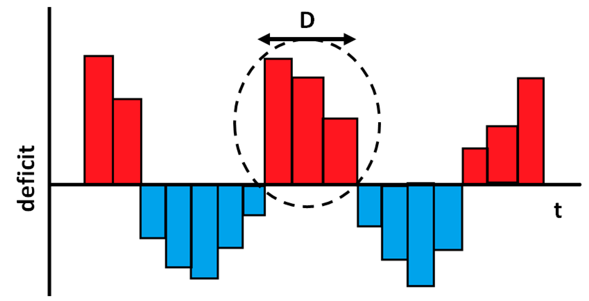
Subsequently, drought events can be obtained from the time series of water deficits using the theory of runs [32]. Yevjevich, [32] defined a drought event as a succession of consecutive periods in which water demand exceeds water supply. A drought event can be characterized by its duration $\left(D\right)$, magnitude $\left(M\right)$, intensity $\left(I\right)$ and frequency (F) [10,32] (Figure 1).

Duration is defined as the number of consecutive months where the amount of water demanded exceeds the amount of water supplied to a given sector. Magnitude or severity is the cumulative deficit over the duration of the drought event defined as:

$$M={\displaystyle \sum }_{j=t}^{t+D-1}\left(d_j\right)$$

(2)

Intensity of drought is the magnitude of a drought event divided by its duration given by:

$$I=\frac{M}{D}$$

(3)

and frequency can be defined as the number of times that a specific drought event occurs in a given period. Frequency can be predicted based on the theoretical probability distribution. The designs of water supply systems are based on historical drought IDF relationships. However, these relationships may need to be modified under the impact of climate change by developing the sub-annual socioeconomic drought IDF curves [17,33].

2.2. Gamma-GPD Mixture Model

Drought events have been modeled by many probabilistic distributions such as Gamma [10,34,35], Exponential [34,35], Normal [8], Log-Normal and Weibull [35]. Gamma distribution is among the most commonly used probability distributions for characterizing drought properties [10,11,34,36,37]. The Gamma distribution has a density function [36] as follows:

$$G\left(x;r,a\right)=\frac{1}{a\Gamma \left(r\right)}{\left(\frac{x}{a}\right)}^{r-1}exp\left(-\frac{x}{a}\right)$$

(4)

where $x$ denotes drought properties, and $r$ and $a$ are the shape and scale parameters, respectively.

Several characteristics motivate the use of the Gamma distribution for describing drought events. First, the distribution is bounded on the left at zero. Thus, it excludes negative values, which is important for drought applications because negative deficit, duration and intensity are impossible. Second, the Gamma distribution is positively skewed with an extended tail to the right. This property is well suited for characterization of droughts with frequent minor and infrequent extreme events. Third, the versatility of the Gamma distribution in taking exponential decay to nearly normal forms lends itself to modeling a range of drought intensity and duration combinations with reasonable accuracy [38].

However, extreme drought events especially under nonstationary conditions may not be adequately characterized by the upper tail of the Gamma distribution. The distribution of drought events will become less positively skewed over time with the increasing occurrence of extreme drought events [23,39]. As the Gamma distribution becomes less positively skewed, the upper tail of the distribution will be insufficient to capture the increasing extreme drought events [38]. Thus, the Gamma distribution may fail to adequately characterize the upper tail of drought events with higher intensities and durations under nonstationary shifts in water supply and demand conditions.

Extreme value analysis (EVA) is increasingly used for robust estimation of extreme events [40]. The Generalized Extreme Value (GEV) approach of Block Maxima (BM) and Generalized Pareto Distribution (GPD) approach of Peak Over Threshold (POT) are two commonly used EVA methods for fitting the extremes of hydrological variables such as those used to characterize drought events [41]. However, the applicability of the GEV distribution by the method of BM is limited for assessment of drought events at sub-annual steps since only one extreme value per year is modeled. Thus, we use the GPD to fit the extreme of sub-annual drought events by applying the POT method [41,42]. The cumulative distribution function (CDF) of the GPD is given by:

$$g_{u,\xi ,\beta }\left(x\right)=\mathrm{Pr}\left(X\le x|X>u\right)=\{\begin{array}{c}1-{\left(1+\xi \frac{x-u}{\beta }\right)}^{-\frac{1}{\xi }} for \xi \ne 0\\ 1-exp\left(-\frac{x-u}{\beta }\right) for \xi =0\end{array}$$

(5)

where $u,\xi$ and $\beta$ are the location (threshold), shape and scale parameters, respectively [40]. The distribution is heavy-tailed when $\xi >0$, medium-tailed when $\xi =0$, and short-tailed with finite upper end point $u-\frac{\beta }{\xi }$ when $\xi <0$ [36]. The threshold should be selected as the GPD location parameter to model statistical properties of events that exceed the threshold.

Here, the Gamma distribution was reconciled with the GPD in a mixture model to simultaneously model the bulk and upper tail of drought events. In this model, values below the GPD threshold (i.e., location parameter) were fitted by the Gamma distribution while values above the threshold were fitted by the GPD (Figure S1). The mixture Gamma-GPD cumulative function ($F$) is given by:

$$F(x|r, a, \xi ,\beta , u, {\varphi }_u)=\{\begin{array}{l}\left(1-{\varphi }_u\right)\frac{G\left(x|r,a\right)}{G\left(u|r,a\right)} x<u\\ \left(1-{\varphi }_u\right)+{\varphi }_u g(x| \xi ,\beta , u) x\ge u\end{array}$$

(6)

where $g(x| \xi ,\beta , u)$ is the unconditional GPD function, $G\left(x|r,a\right)$ is the Gamma distribution function, $u$ is the GPD location parameter (threshold), and ${\varphi }_u$ is the probability of $x$ being above the threshold [25,43]. Hence, the mixture model $F(x|r, a, \xi ,\beta , u, {\varphi }_u)$ can be used to model the distribution of both non-extreme and extreme droughts intensity and duration by inserting Equations (4) and (5) into Equation (6).

It should be noted that some previous studies have applied mixture distribution models to combine different distributions to simultaneously model both central and tail. However, the fit of mixture models has not been investigated in terms of sub-annual socioeconomic drought properties. It can be suggested that mixture models lead to better estimation of return periods of both minor and extreme drought events.

2.3. Joint Probability Distribution of Drought Intensity and Duration

The mixture Gamma-GPD model is used in this study to determine sub-annual socioeconomic drought IDF relationships. Drought intensity, duration, and frequency properties are correlated random variables. The joint probability distribution of drought events for intensity $\mathrm{I}>{\mathrm{I}}_0$ and duration $\mathrm{D}>{\mathrm{D}}_0$ can be constructed by the product of the conditional distribution of drought intensity for a given duration and the marginal distribution of drought duration as follows:

$$P (\mathrm{I}>{\mathrm{I}}_0 \cap \mathrm{D}>{\mathrm{D}}_0)=P (\mathrm{I}>{\mathrm{I}}_0 | \mathrm{D}>{\mathrm{D}}_0) .P (\mathrm{D}>{\mathrm{D}}_0)$$

(7)

where ${\mathrm{D}}_0$ and ${\mathrm{I}}_0$ denote any given values of duration and intensity, respectively. The term $P (\mathrm{I}>{\mathrm{I}}_0$|$\mathrm{D}>{\mathrm{D}}_0)$ is the conditional probability of $\mathrm{I}>{\mathrm{I}}_0$ given $\mathrm{D}>{\mathrm{D}}_0$, and $P (\mathrm{D}>{\mathrm{D}}_0)$ is the marginal probability of drought with $\mathrm{D}>{\mathrm{D}}_0$. The marginal probability of $\mathrm{D}>{\mathrm{D}}_0$ from the mixture Gamma-GPD is given by:

$$P \left(\mathrm{D}>{\mathrm{D}}_0\right)=F(\mathrm{D}>{\mathrm{D}}_0)=\{\begin{array}{c}\left(1-{\varphi }_u\right)\frac{G\left(\mathrm{D}>{\mathrm{D}}_0|r,a\right)}{G\left(\mathrm{u}|r,a\right)} x<u\\ \left(1-{\varphi }_u\right)+{\varphi }_u g(D>{\mathrm{D}}_0| \xi ,\beta , u) x\ge u\end{array}$$

(8)

The conditional probability of $P (\mathrm{I}>{\mathrm{I}}_0$|$\mathrm{D}>{\mathrm{D}}_0)$ can be determined in the same way considering that the mixture model should be fitted to just drought events with $\mathrm{D}>{\mathrm{D}}_0$ as follows:

$$P \left(\mathrm{I}>{\mathrm{I}}_0| \mathrm{D}>{\mathrm{D}}_0\right)=F(\mathrm{I}>{\mathrm{I}}_0|\mathrm{D}>{\mathrm{D}}_0)$$

(9)

Finally, the joint probability distribution of drought intensity and duration can be computed by inserting Equations (8) and (9) into Equation (7) and assuming drought events follow the mixture Gamma-GPD model. Thus, Equation (7) can be used to improve estimation of drought intensity, duration and frequency relationships by assuming that both marginal and conditional probabilities are Gamma-GPD distributed.

2.4. Parameter Estimation and Goodness-of-fit Tests

The proposed mixture Gamma-GPD distribution was linked with population and climate change models in this study as an effective way to address shifts in drought properties under a changing environment. Then, the applicability of the proposed mixture Gamma-GPD distribution was investigated compared to classic families of probabilistic distributions, especially under considerable shifts in water supply and demand conditions. Nonstationary conditions arising from sub-annual changes in supply and demand are represented by time-varying parameters. Mixture Gamma-GPD model parameters were re-estimated as a function of time using 30-year overlapping moving windows on the nonstationary time series of drought events.

In this study, the nonstationary climate data were obtained from the CMIP5 projections, and subsequently downscaled for meteorological stations in the region using a quantile-based empirical-statistical error correction method and a subsequent temporal (i.e., monthly to daily) downscaling procedure [44]. Then, the nonstationary water demand and supply time series for the 1985–2065 were estimated using the Integrated Urban Water Model (IUWM) and the Soil and Water Assessment Tool (SWAT), respectively. The proposed mixture model holds the versatility to account for these changes in drought properties over time.

The location parameter of the GPD should be estimated to define the threshold between the bulk and tail distributions. The appropriate threshold is the location at which the mean residual life plot is approximately linear [25,26]. It should be high enough to follow a GPD. In addition, the sample size should be large enough for inference. The other parameters of Gamma-GPD mixture model were estimated using the maximum likelihood estimator (MLE) in MATLAB (MathWorks, Natick, MA, USA).

Several goodness-of-fit tests were applied to assess how well the proposed mixture Gamma-GPD model fits a set of drought intensities and durations. Here, the performance of the mixture model was evaluated using the chi-square goodness-of-fit test, root-mean-square error (RMSE), and the coefficient of determination. The performance of the model was compared with the performance of other standard distributions. Goodness-of-fit tests are frequently used as a measure of the differences between values predicted by a model or an estimator and the observed values [45,46]. The smallest RMSE and Chi-square and largest R-squared indicate the model with the best performance.

2.5. Return Period

Return periods of drought events are often used to design the capacity of water supply systems [10]. The return period of droughts with intensity greater than or equal to a target ($\mathrm{I}>{\mathrm{I}}_0$) was derived as a function of the expected drought interarrival time and cumulative drought intensity distribution function, expressed as:

$$T_{\mathrm{I}>{\mathrm{I}}_0| \mathrm{D}>{\mathrm{D}}_0}=\frac{E\left(\mathrm{D}>{\mathrm{D}}_0\right)}{P (\mathrm{I}>{\mathrm{I}}_0| \mathrm{D}>{\mathrm{D}}_0)}\times \frac{1}{P\left(\mathrm{D}>{\mathrm{D}}_0\right)}=\frac{E\left(\mathrm{D}>{\mathrm{D}}_0\right)}{P (\mathrm{I}>{\mathrm{I}}_0\cap \mathrm{D}>{\mathrm{D}}_0)}$$

(10)

where $E\left(\mathrm{D}>{\mathrm{D}}_0\right)$ is the expected drought interarrival time with $\mathrm{D}>{\mathrm{D}}_0$, which can be estimated from observed droughts, and $P (\mathrm{I}>{\mathrm{I}}_0\cap \mathrm{D}>{\mathrm{D}}_0)$ can be obtained from Equation (7). The expected value of the interarrival time between two successive drought events with a certain duration or greater is given by [35,47]:

$$E\left(\mathrm{D}>{\mathrm{D}}_0\right)=E\left({\displaystyle \sum }_{i=1}^N{\mathrm{DI}}_{\mathrm{i}}\right)$$

(11)

where ${\mathrm{DI}}_{\mathrm{i}}$ is drought interarrival time between two successive drought events with a certain duration or greater, and $N$ is the number of drought events equal to or greater than a certain duration.

2.6. Drought Risk and Amplification Factor

The risk of failure over an n-year design or assessment period may be written as [17,48]:

$$Risk (\mathrm{I}>{\mathrm{I}}_0| \mathrm{D}>{\mathrm{D}}_0)=1-{\left(1-\frac{1}{T_{\mathrm{I}>{\mathrm{I}}_0| \mathrm{D}>{\mathrm{D}}_0}}\right)}^n$$

(12)

where $T_{\mathrm{I}>{\mathrm{I}}_0| \mathrm{D}>{\mathrm{D}}_0}$ is the return period of droughts with intensity and duration greater than or equal to a certain threshold ($\mathrm{I}>{\mathrm{I}}_0, D>D_0$) and n is the project life in years. Nonstationarity in drought risk projection can be accounted for by estimating changes in the exceedance probability of the mixture model using time-varying parameters.

In addition, the change in drought frequencies under nonstationary conditions can be quantified by dividing the exceedance probability of a given drought event in the future to the current condition as:

$$Amplification Factor \left(AF\right)=\frac{P_t\left(I>I_0\right)}{P_C\left(I>I_0\right)}$$

(13)

where $AF$ is the frequency amplification factor of drought with $I>I_0$, and $P_C\left(I>I_0\right)$ and $P_t\left(I>I_0\right)$ are the exceedance probability of drought events with $I>I_0$ for current and future conditions, respectively. The drought events with higher frequency amplification factor are more sensitive to nonstationary conditions.

2.7. Global Sensitivity Analysis

A global sensitivity analysis was performed to simultaneously assess both relative contributions and interactions between each of the individual mixture model parameters. Several techniques have been commonly used to execute global sensitivity analysis. In this study, the method of Sobol [49] was applied using the SIMLAB software package [50]. Sobol decomposes the variance of the output into fractions, which can be allocated to individual inputs. Both relative contributions and interactions of individual inputs were calculated using the first-order and total-order sensitivity indices. Sensitivity indices are defined to measure the importance of variables. The distribution of the mixture model parameters was assumed to be uniform. The selected ranges of mixture model parameters are shown in Table S1 based on the observed data and their intervals.

First-order sensitivity indices were used to assess the contribution of an individual parameter to the output variance. Parameters with the greater first-order sensitivity indices are more critical for the model. Figure 2 (left-panel) and Table S2 illustrate the first order sensitivity indices of model parameters to return period of drought with duration equal or greater than one month. Below the threshold (non-extreme drought events), the mixture model is governed by Gamma parameters. The drought return period is more sensitive to the Gamma shape parameter than the Gamma scale parameter. Above the threshold (extreme drought events), the mixture model is governed by GPD parameters. The drought return period is respectively sensitive to the location, scale, and shape parameters of the GPD.

Total-order sensitivity indices were used to assess the interaction between each of the input variables. Changes in the total order sensitivity indices are presented in Table S3 and Figure 2 (right-panel). GPD scale and GPD shape parameters are more critical when the total-order sensitivity indices were considered. This indicates that shape and scale parameters of GPD have significant interactions with other parameters.

Figure 3 illustrates the interaction between the GPD shape and Gamma shape parameters with GPD location (threshold) parameter. Below the threshold (Figure 3 left-panel), as Gamma shape parameter increases, sensitivity of drought return period to change in GPD location parameter increases. Conversely, as GPD location parameter increases, the sensitivity of drought return period to change in the Gamma shape parameter increases. Above the threshold (Figure 3 right-panel), the sensitivity of drought return period to change in the GPD location parameter decreases. Conversely, as the GPD location parameter increases, the sensitivity of drought return period to the change in Gamma shape parameter decreases.

3. Application and Discussion

The proposed probabilistic approach was demonstrated for the City of Fort Collins (Colorado, USA) water supply system (Figure S2) as a test case to investigate the applicability of the framework under considerable shifts in water supply and water demand conditions. Climate, water supply, and water demand for Fort Collins were projected out to 2065 under the hot-dry scenario to assess the capacity to improve characterization of sub-annual socioeconomic drought IDF relationships under significant shifts in water supply and demand conditions. The 1986–2015 period was used to represent “current” conditions and the 2035–2065 period represented the “mid-century” conditions. It should be emphasized that assessing various aspects of future drought impacts on the City of Fort Collins is not the purpose of this study. In fact, this study used the City of Fort Collins as a test case to demonstrate the application of the proposed approach under nonstationary conditions.

Fort Collins is in the semi-arid American West, which is prone to extended droughts. It lies within the Cache la Poudre (CLP) watershed in Northcentral Colorado. Currently, a drought event is defined as one or more years of below average annual runoff in the CLP River [51]. An exceptionally severe drought was reported in Fort Collins from September 2001 to August 2002. Over the last decades, CLP River discharge has been below average in most years, and the city has been experiencing water shortage conditions since 2000. In addition, high levels of population growth are projected within the CLP watershed, compounding the water shortage problems [51].

3.1. Future Climate Scenarios

Changes in precipitation and temperature for the CLP watershed were estimated under the representative concentration pathway (RCP) 8.5 and a hot-dry scenario described below. This combination was chosen to represent a worst-case condition for the region. Observed daily temperature and precipitation data were collected from the Global Historical Climatology Network (GHCN), the Colorado Agricultural Meteorological Network (CoAgMet), and Northern Colorado Water Conservancy District (NCWCD). Missing data were filled using auxiliary information obtained from nearby stations based on the probability of rainy days, R-Squared and Jaccard index between the two nearest stations.

Future monthly climate data were obtained from CMIP5 projections [52]. Subsequently, data were statistically downscaled for meteorological stations in the region using a quantile-based empirical-statistical error correction method [44]. A downscaling procedure was performed to obtain daily climate information from downscaled monthly data. Two hundred and thirty downscaled climate models were classified into hot-dry, hot-wet, warm-dry, warm-wet, and median categories based on the difference in current and future temperature and precipitation (Figure S3).

Changes in precipitation and minimum temperature in Fort Collins under the median of 230 climate models are shown in Figure 4a,b, respectively. The average changes in minimum temperature for RCP 2.6, 4.5, 6.0 and 8.5 are also shown in Figure 4c. Climate anomalies represent differences between the mid-century and current conditions. The kriging method in ArcGIS was applied to the spatial interpolation of precipitation and temperature anomaly records in the CLP watershed.

For the median of 230 climate models (Figure 4), temperature consistently is expected to increase across the watershed. In addition, the rate of warming tends to increase with elevation, indicating that high-mountain environments of the Colorado Rocky Mountains will experience rapid changes in temperature. However, a relatively small increase in precipitation was projected, particularly in higher elevation areas.

In this study, the statistically downscaled ‘ipsl-cm5a-mr’ scenario was selected from the hot-dry category with RCP 8.5 to represent the worst-case scenario for the mid-century conditions. This scenario was selected in order to assess significance and applicability of the proposed framework under considerable shifts in water supply and demand conditions. Figures S4 and S5 show changes in precipitation and temperature for the hot-dry scenario from current conditions to mid-century conditions.

3.2. Water Supply Assessment

The City of Fort Collins receives native water from the Cache la Poudre (CLP) River and imported water from Horsetooth Reservoir as part of the Colorado Big Thomson (CBT) project. According to the Fort Collins Water Supply and Demand Management Policy Revision Report [51], the amount of usable water from the Poudre River depends on factors such as water demand, dry-year yields and exchange potential. In addition, water deliveries from the Colorado Big Thompson system to the city of Fort Collins depend on an annual quota set by Northern Water each year ranging from 50% to 100% of annual yields [51]. In this study, the potential amount of water supplied to the City of Fort Collins in the future was calculated assuming that the historical coefficients of water deliveries from the CLP River will be preserved and the City owns the potential amount of water from the Horsetooth Reservoir as the most flexible source to fill gaps from other sources.

Changes in water yield in the CLP River at the Mouth of Canyon Station (National Water Information System (NWIS), 2019) was evaluated using the Soil and Water Assessment Tool (SWAT) [53]. SWAT is a comprehensive, distributed-parameter, process-based hydrologic model that has been used extensively to assess the hydrologic response to changes in climate and land use at a variety of scales [54,55,56,57]. The model was calibrated to historic naturalized flow data at multiple locations within the watershed [58]. The calibrated model was driven by projected alternative future climates for the region to obtain monthly discharge at the City of Fort Collins water intake facilities on the CLP River.

3.3. Water Demand Assessment

Municipal water demand under climate, population, and water demand management scenarios was estimated using the Integrated Urban Water Demand Model (IUWM). IUWM is a mass balance model that simulates water demand and wastewater production associated with urban water demand management strategies. The model simulates municipal water demand through use of population, household, land cover and climate data. The model was calibrated and tested for the City of Fort Collins with options for assessing demand management scenarios based on the projected population, temperature and precipitation [59]. The model was driven with future climate scenarios to obtain monthly total water use for the City of Fort Collins under nonstationary conditions. Population and household information were obtained from the U.S. Census Bureau [60]. Population growth projections were based on those reported in AMEC Environment and Infrastructure [51] with a projected population of 165,000 by the middle of century.

Figure 5 provides 12-month average of projected water supply and water demand for the City of Fort Collins under the hot-dry scenario. The balance between water supply and water demand becomes more unequal by the middle of the century under rapid climate changes and population growth. This situation can lead to considerable shifts in socioeconomic drought distributions. Thus, applicability of classic families of probabilistic distributions can be assessed compared to the mixture Gamma-GPD distribution in rapidly changing environment.

3.4. Water Deficit Record Extension

Extreme drought events are usually infrequent and insufficient for fitting to a GPD model [10,61]. To create a statistically large monthly water deficit sample, the autoregressive (AR) time series model was used. The AR model of order $p$, AR ($p$), is a time series defined by [10]:

$$y_t=c+{\displaystyle \sum }_{i=1}^p{\varphi }_{\mathrm{i}} \left(y_{t-i}\right)+{\epsilon }_t$$

(14)

with lagged values of $y_t$ as predictors where ${\epsilon }_t$ is an uncorrelated normal random variable with mean zero and variance ${\sigma }_{\epsilon }^2$, and ${\varphi }_i$, and $c$ are the parameters of the model. The fourth-order autoregressive model was found to be effective for simulating a synthetic 67200-month deficits sample for the city of Fort Collins. This extended sample was used to determine intensity, duration, and frequency of drought events for the study system. The relative frequency distribution of positive drought deficits ($d>0$) from the historical record and the generated sample are shown in Figure 6. Furthermore, the synthetic sample was tested by comparing statistical properties of original data versus generated data using AR model for all deficits (

Table 1. Statistical properties of original data versus generated data for city of Fort Collins.

Statistics	Original Data	Generated Data
Single Deficit
Min (million cubic meter)	−3.851	−3.772
Max (million cubic meter)	4.214	4.170
Mean (million cubic meter)	0.173	0.173
Standard deviation	1.114	1.054
Coefficient of variation	6.422	6.070
Severity
Mean (million cubic meter)	8.823	7.644
Standard deviation	22.380	22.323
Coefficient of variation	2.536	2.920
Intensity
Mean (million cubic meter per month)	0.545	0.582
Standard deviation	0.379	0.335
Coefficient of variation	0.695	0.576
Duration
Mean (month)	9.974	8.373
Standard deviation	18.576	17.456
Coefficient of variation	1.862	2.084

).

3.5. Importance of Nonstationarity Assumptions in Both Water Supply and Demand Conditions

While all types of droughts originate from a deficiency in water supplies, drought properties would not depend on only water supply conditions. Climate changes and population growth can lead to nonstationary conditions in both water supply and water demand conditions. Thus, definition and characterization of drought events that consider shifts in both water supply and demand are essential to account for a changing environment. However, most previous studies have defined socioeconomic drought only in terms of deficiencies in water supply systems [14,16].

Table 2. Impacts of shifts in both water supply and water demand on drought properties.

Drought Properties	Shifts in Demand	Shifts in Supply	Shifts in Supply and Demand
Magnitude (mcm)	1.03	1.74	8.20
Duration (month)	4	3.30	9.38
Intensity (mcm/m)	0.22	0.40	0.53
Maximum water deficit (mcm)	0.32	0.68	1.04

shows the impact of nonstationary assumptions in both water supply and demand conditions on drought properties compared to shifts in only water supply or water demand conditions. The average drought magnitude, duration, intensity, and maximum monthly water deficit are determined under shifts in (1) only demand conditions; (2) only supply conditions; and (3) both supply and demand conditions. While the average magnitude and duration of drought events considerably increase by assuming shifts in both water supply and demand conditions, the average drought intensity increases slightly. Based on the drought intensity definition (magnitude/duration), minor changes in drought intensity can be justified considering that intensity is a normalized value (water deficit per month). However, maximum monthly deficit will increase to 1.04 (mcm/month).

Table 2 provides a general understanding of how shifts in water supply and water demand contribute to affect drought properties in the selected case-study. Under constant water demand assumption, the average magnitude, intensity, and maximum monthly water deficit are higher than the constant water supply assumption. Table 2 highlights that change in water supply may have higher impacts on drought magnitude and intensity compared to changes in water demand. It should be noted that these results are case-study specific and depend on the selected scenario.

3.6. Importance of Socioeconomic Drought Assessment at a Sub-annual Scale

Drought is traditionally defined as a climate phenomenon that takes many years. Most studies have characterized drought at annual scale. However, population growth and climate change can lead to higher interannual variability of water supply and water demand. Thus, characterization of socioeconomic drought properties at a sub-annual scale is needed in a changing environment. Figure 7 shows changes in drought intensity for D < 12 months from current conditions to future conditions. Intensity of within-year drought increases due to increases in interannual variability of water supply and demand conditions.

In addition, characterization of socioeconomic drought at a sub-annual scale makes a significant difference in the definition of drought duration. For example, droughts with duration equal to 24 months (D = 24 months) are not equivalent to droughts with durations equal to 2 years (D = 2 years). In fact, droughts with D = 24 months mean that there are 24 consecutive months in which monthly water demand is greater than monthly water supply. However, droughts with D = 2 years mean that there are two consecutive years in which total annual water demand is greater than total annual water supply. Thus, even during a two-year drought, there may be months with water surplus. As a result, characterization of drought events at a sub-annual scale can help to identify months with water surplus that can lead to enhanced decision-making in water resource planning and management.

3.7. Importance of Applying Mixture Gamma-GPD Distribution under Nonstationary Conditions

The Mixture Gamma-GPD distribution was used to estimate the frequency of socioeconomic drought intensity and duration at a sub-annual scale for the City of Fort Collins. In this study, the threshold related to the 95th sample percentile [41,42,43] was chosen, which was supported by using the mean excess plots (Figures S6 and S7) as a graphical diagnostics method.

The model evaluation criteria including Chi-square, RMSE, and R-squared are summarized in

Table 3. The goodness of fit of various models under current conditions (drought intensity).

Distribution	R-squared	RMSE	Chi-Square
Exponential	0.7104	0.14	86.1532
Normal	−16.8745	0.5912	333.0102
Log-Normal	0.6728	0.1414	42.3706
Weibull	0.6147	0.1749	186.4215
Gamma	0.9447	0.0652	10.9257
Gamma-GPD	0.9746	0.046	10.8214

,

Table 4. The goodness of fit of various models under mid-century conditions (drought intensity).

Distribution	R-squared	RMSE	Chi-Square
Exponential	0.2735	0.273	274.5355
Normal	−5.5551	0.6131	303.6521
Log-Normal	0.5086	0.2233	71.4617
Weibull	0.511	0.2145	321.0255
Gamma	0.8736	0.1207	24.9927
Gamma-GPD	0.945	0.0808	22.6967

,

Table 5. The goodness of fit of various models under current conditions (drought duration).

Distribution	R-squared	RMSE	Chi-Square
Exponential	0.701	7.2617	97.2247
Normal	−1.0406	19.7033	2393.4
Log-Normal	0.6563	10.6014	213.2408
Weibull	0.6739	7.5839	107.309
Gamma	0.6476	4.2436	35.82
Gamma-GPD	0.9488	1.6173	7.46

and

Table 6. The goodness of fit of various models under mid-century conditions (drought duration).

Distribution	R-squared	RMSE	Chi-Square
Exponential	0.5314	14.9834	440.1007
Normal	−1.0788	37.6708	9787.0
Log-Normal	0.3578	25.6947	1271.9
Weibull	0.7345	10.6867	201.576
Gamma	0.7705	5.01	47.09
Gamma-GPD	0.957	2.147	13.20

for Exponential, Normal, Log-Normal, Weibull, Gamma and Gamma-GPD distributions under current and future conditions. Most classic families of distributions have better fit under current conditions compared to mid-century conditions. This finding indicates that the most standard probabilistic distributions will be insufficient to capture both bulk and tail of droughts distribution under shifts in drought properties by the mid-century. In addition, goodness of fit tests quantitively demonstrate that the standard Gamma distribution better fits to sub-annual socioeconomic drought durations and intensities compared to other probabilistic distributions for both current and mid-century conditions. However, the mixture Gamma-GPD distribution leads to improved estimation of drought frequency compared to Gamma and other probabilistic distributions for both drought duration and intensity under current and future conditions. The approach improves the capacity to simultaneously characterize within-year and multi-year socioeconomics droughts.

Figure 8 shows the quantile-quantile (QQ) plots of both Gamma-GPD and Gamma distributions for the current (1986–2015) and future (2035–2065) conditions. The Gamma-GPD model substantially improves characterization of socioeconomic drought intensity-duration relationships, particularly under nonstationary conditions. The proposed mixture model consistently provides a better fit to data compared to the standard Gamma distribution as QQ plots indicate.

While the Gamma distribution (red plus sign) seems to be adequate for drought events with smaller duration and intensities (non-extreme droughts), it tends to be inadequate for droughts with larger duration and higher intensity (extreme droughts) by deviating from the reference line. However, the Gamma –GPD distribution (blue circle sign) enhances the characterization of extreme drought events by converging to the reference line.

Changes in the probability distribution functions of drought durations with intensity greater than zero (all drought events) are shown in Figure 9 left-panel. The GPD of drought durations is short-tailed ($\xi <0)$ under the current condition but becomes heavy-tailed $(\xi >0)$ during the mid-century period, meaning that the duration of drought events will increase by the middle of century. The scale parameter of the Gamma distribution for drought duration is increasing, which means that the variability of drought durations will increase in the middle of century.

Drought intensities with duration greater than one month (all drought events) are depicted in the right panel of Figure 9. The GPD location parameter was increased over time from 1.0 to 1.22 mcm (million cubic meter) per month, meaning that drought events that are currently characterized as extreme events become non-extreme events in the middle of century. The scale parameter of the Gamma distribution for drought intensity also increases, indicating that the variability of drought intensity will increase. Changes in climate and population alter the distribution of both drought durations and intensities over time. There may be a discontinuity in the density at the threshold; however, the mixture probability distribution will be continuous.

3.8. Application of Sub-annual Socioeconomic Drought IDF Relationships in a Changing Environment

How socioeconomic drought properties will change in the future is one of the key research questions in water resource management and planning. This section discusses the practicality of the proposed approach to update drought IDF curves and designed drought event for water supply systems. These critical factors can affect water supply and demand management policies and practices. First, we assess changes in sub-annual socioeconomic drought IDF curves for the City of Fort Collins under significant shifts in water supply and demand. Improving the estimation of socioeconomic drought IDF curves under nonstationary conditions can play an important role in the design of water supply systems. Second, we assess changes in the designed drought event for the City of Fort Collins water supply systems under nonstationary conditions.

3.8.1. Sub-annual Socioeconomic IDF Curves in a Changing Environment

IDF curves are commonly applied for the design of water resource systems such as municipal storm-water drainage systems. However, studies that discuss methods for assessing changes in IDF relationships of drought events are limited [17,33]. IDF curves were obtained through frequency analysis of drought events. Drought Intensity and duration time series were computed for overlapping 30-year moving windows to calculate changes in drought properties due to nonstationary water supply and demand. Changes in the parameters of the mixture model were estimated using overlapping 30-year moving windows and assuming the parameters are time-varying. Figure 10 illustrates changes in the projected drought durations (left panel) and drought intensities (right panel) for the Fort Collins water supply system under the hot-dry scenario. Drought events with higher intensity have longer duration. Similarly, drought events with longer duration have higher intensities. The results also indicate that drought events with longer durations and higher intensities will be more frequent under the projected scenario.

The expected value of interarrival time between two successive drought events is shown in Figure 11. The occurrence probability of drought events is expected to change significantly over time under the hot-dry scenario. Drought events with longer duration have higher changes in the expected interarrival time.

The amplification factor was also calculated for different drought durations and intensities. Multi-year and higher intensity droughts (extreme droughts) tend to be more sensitive to nonstationary conditions than droughts with duration less than a year (Figure 12). The results point to a substantial increase in the occurrence of extreme events from 2005 to 2060 (i.e., drought events with higher intensities and longer durations). Socioeconomic droughts with longer duration will have higher likelihood of occurrence in the mid-century compared to current conditions.

Then, the marginal and conditional probabilities of drought events as well as the joint probability distribution of drought events for intensity and duration greater than or equal to a target ($\mathrm{I}>{\mathrm{I}}_0$,$\mathrm{D}>{\mathrm{D}}_0$) were computed. Drought frequency analysis was performed for each set of drought duration to determine the exceedance probability of drought intensity.

Figure 13 depicts the drought IDF curves with durations greater than 1, 6, 12, 24 and 36 months under nonstationary conditions for both current and future conditions. The results indicate that current IDF curves substantially underestimate extreme drought events. For example, the return periods of drought events with durations greater than 24 and 36 months decrease to less than 1000 years in the future. In addition, the IDF curves for both current and future conditions indicate that the drought events with shorter durations tend to have higher intensities. Thus, current drought IDF curves seem inadequate for the design and management of water supply infrastructure under considerable shifts in water supply and demand conditions. The proposed probabilistic approach should be applied for improved characterization of future IDF relationships, particularly for extreme socioeconomic droughts.

3.8.2. Changes in the Designed Drought Event for Water Supply Systems

Based on the Fort Collins Water Supply and Demand Management Policy Revision Report [51], the City’s water utility tries to maintain water supplies sufficient to meet demands during at least a 1-in-50 year drought. A 1-in-50 year drought is a drought event that occurs once every 50 years, on average [51]. Figure 14 shows the risk of 1-in-50 year drought events with different durations for current and mid-century conditions. 1-in-50 year drought risk decreases as drought intensity increases. The model used here shows that drought events with longer durations are more likely in the middle of the century compared to current conditions. Therefore, the design drought event for the City’s water supply system should be updated according to the accepted risk for the middle of the century.

The proposed mixture model thus leads to enhanced assessment of sub-annual socioeconomic drought IDF relationships by simultaneously capturing non-extreme and extreme droughts under annual and interannual shifts in water supply and demand trends. Design of water supply systems by using the proposed probabilistic approach can improve the capacity of city water managers to adequately implement drought adaptation strategies such as water supply development, water demand management, and conservation [4,15,18,42]. Updating drought IDF curves and designed drought events help decision makers and system designers to understand uncertainties under climate change and population growth and develop climate adaptation strategies to increase resilience and flexibility of water supply systems [62].

4. Conclusions

In rapidly urbanizing areas, population growth along with changes in climate can lead to nonstationary drought conditions where water demand exceeds water supply. Three important considerations were addressed in this study under growing unequal balance between water supply and water demand. First, an improved socioeconomic drought assessment can be characterized by assuming shifts in both water supply and demand conditions. Second, assessing the drought properties at a sub-annual scale is essential toward improved water resource management. Third, a mixture distribution is needed to account for considerable shifts in both water supply and water demand conditions. These considerations are addressed in this study to update drought IDF relationships using defined sub-annual socioeconomic drought terminology.

We outlined a statistically coherent probabilistic approach for assessing sub-annual socioeconomic drought IDF properties in a changing environment, while considering shifts in both water supply and water demand regimes to cope with climate changes and population growth. A mixture Gamma-GPD probability model was proposed to simultaneously represent the bulk and tail of drought events. The standard probabilistic distributions were found to be insufficient for modeling extreme socioeconomic droughts with longer duration and higher intensity especially in a rapidly changing environment. The proposed mixture model improved characterization of socioeconomic drought intensity, duration and frequency relationships at sub-annual time scales, particularly under significant shifts in water supply and demand trends. Under nonstationary water supply and demand conditions, current extreme and infrequent drought events may become more frequent. Thus, more attention should be given to the enhanced characterization of extreme socioeconomic droughts. The model can enhance the capacity to address challenges with interannual variability of water supply and demands under nonstationary conditions.

Application of the framework was demonstrated for the City of Fort Collins, Colorado, water supply system. Climate changes were derived from GCM projections, and supply and growing demand were calculated using SWAT and IUWM models respectively by considering population growth and future climate scenarios. The hot-dry scenario was selected to represent the worst-case conditions for nonstationary water supply and demand. Assessments of sub-annual drought frequency for City of Fort Collins indicate that climate change and population growth will significantly affect the vulnerability of municipal water supply systems to shortage. The proposed mixture model improved the projection of sub-annual socioeconomic drought intensities and durations, particularly for extreme drought events. In the case of the City of Fort Collins, the 1-in-50 year drought risk increases from current conditions by the mid-century, indicating that the City will experience socioeconomic droughts with higher intensity and longer duration. Moreover, drought events with longer duration have higher risk in the middle of century compared to current conditions. Drought events with longer duration are more sensitive to non-stationary conditions.

This study provides a framework to statistically assess impacts of large shifts in water supply and demand on sub-annual socioeconomic droughts. However, global assessment of sub-annual socioeconomic drought propagation under various anthropogenic water demand scenarios, climate change projections, and water supply infrastructure designed is needed.

The findings of this study can be applied to update socioeconomic drought IDF properties that are used to assess water storage, to plan water supply systems under nonstationary conditions, and to optimize water institutions and management including water rights in the American West. Finally, the methodology developed in this study can be applied for other sectors such as agriculture to evaluate the impacts of climate change, land-use change, and socioeconomic drivers on water shortage.

References

- Naz, B.S.; Kao, S.C.; Ashfaq, M.; Rastogi, D.; Mei, R.; Bowling, L.C. Regional hydrologic response to climate change in the conterminous United States using high-resolution hydroclimate simulations. Glob. Planet. Chang. 2016, 143, 100–117. [Google Scholar] [CrossRef] [Green Version]
- Wang, X.J.; Zhang, J.Y.; Shahid, S.; Guan, E.H.; Wu, Y.X.; Gao, J.; He, R.M. Adaptation to climate change impacts on water demand. Mitig. Adapt. Strateg. Glob. Chang. 2016, 21, 81–99. [Google Scholar] [CrossRef]
- Mahat, V.; Ramírez, J.A.; Brown, T.C. Twenty-First-Century Climate in CMIP5 Simulations: Implications for Snow and Water Yield across the Contiguous United States. J. Hydrometeorol. 2017, 18, 2079–2099. [Google Scholar] [CrossRef]
- Brown, T.C.; Mahat, V.; Ramirez, J.A. Adaptation to Future Water Shortages in the United States Caused by Population Growth and Climate Change. Earth’s Futur. 2019, 7, 219–234. [Google Scholar] [CrossRef] [Green Version]
- Hemmati, M.; Ellingwood, B.R.; Mahmoud, H.N. The Role of Urban Growth in Resilience of Communities Under Flood Risk. Earth’s Futur. 2020, 8, 1–14. [Google Scholar] [CrossRef] [Green Version]
- Mehran, A.; Mazdiyasni, O.; Aghakouchak, A. A hybrid framework for assessing socioeconomic drought: Linking. J. Geophys. Res. Atmos. 2015, 1–14. [Google Scholar] [CrossRef]
- Rajsekhar, D.; Singh, V.P.; Mishra, A.K. Integrated drought causality, hazard, and vulnerability assessment for future socioeconomic scenarios: An information theory perspective. J. Geophys. Res. 2015, 120, 6346–6378. [Google Scholar] [CrossRef]
- Foti, R.; Ramirez, J.A.; Brown, T.C. A probabilistic framework for assessing vulnerability to climate variability and change: The case of the US water supply system. Clim. Chang. 2014, 125, 413–427. [Google Scholar] [CrossRef]
- Hao, Z.; Singh, V.P.; Xia, Y. Seasonal Drought Prediction: Advances, Challenges, and Future Prospects. Rev. Geophys. 2018, 56, 108–141. [Google Scholar] [CrossRef] [Green Version]
- Salas, J.D.; Fu, C.; Cancelliere, A.; Dustin, D.; Bode, D.; Pineda, A.; Vincent, E. Characterizing the Severity and Risk of Drought in the Poudre River, Colorado. J. Water Resour. Plan. Manag. 2005, 131, 383–393. [Google Scholar] [CrossRef]
- Mishra, A.K.; Singh, V.P. A review of drought concepts. J. Hydrol. 2010, 391, 202–216. [Google Scholar] [CrossRef]
- Huang, S.; Huang, Q.; Leng, G.; Liu, S. A nonparametric multivariate standardized drought index for characterizing socioeconomic drought: A case study in the Heihe River Basin. J. Hydrol. 2016, 542, 875–883. [Google Scholar] [CrossRef]
- Zhao, M.; Huang, S.; Huang, Q.; Wang, H.; Leng, G.; Xie, Y. Assessing socio-economic drought evolution characteristics and their possible meteorological driving force. Geomatics. Nat. Hazards Risk 2019, 10, 1084–1101. [Google Scholar] [CrossRef] [Green Version]
- Guo, Y.; Huang, S.; Huang, Q.; Wang, H.; Fang, W.; Yang, Y.; Wang, L. Assessing socioeconomic drought based on an improved Multivariate Standardized Reliability and Resilience Index. J. Hydrol. 2019, 568, 904–918. [Google Scholar] [CrossRef]
- Warziniack, T.; Brown, T.C. The importance of municipal and agricultural demands in future water shortages in the United States. Environ. Res. Lett. 2019, 14, 084036. [Google Scholar] [CrossRef]
- Tu, X.; Wu, H.; Singh, V.P.; Chen, X.; Lin, K.; Xie, Y. Multivariate design of socioeconomic drought and impact of water reservoirs. J. Hydrol. 2018, 566, 192–204. [Google Scholar] [CrossRef]
- Salas, J.D.; Obeysekera, J.; Vogel, R.M. Techniques for assessing water infrastructure for nonstationary extreme events: A review. Hydrol. Sci. J. 2018, 63, 325–352. [Google Scholar] [CrossRef]
- Gutzler, D.S.; Nims, J.S. Interannual Variability of Water Demand and Summer Climate in Albuquerque, New Mexico. J. Appl. Meteorol. 2006, 44, 1777–1787. [Google Scholar] [CrossRef]
- Yu, P.S.; Yang, T.C.; Kuo, C.M.; Wang, Y.T. A stochastic approach for seasonal water-shortage probability forecasting based on seasonal weather outlook. Water Resour. Manag. 2014, 28, 3905–3920. [Google Scholar] [CrossRef]
- Jaeger, W.K.; Amos, A.; Bigelow, D.P.; Chang, H.; Conklin, D.R.; Haggerty, R.; Langpap, C.; Moore, K.; Mote, P.W.; Nolin, A.W.; et al. Finding water scarcity amid abundance using human–natural system models. Proc. Natl. Acad. Sci. USA 2017, 114, 11884–11889. [Google Scholar] [CrossRef] [Green Version]
- Evans, R.G.; Sadler, E.J. Methods and technologies to improve efficiency of water use. Water Resour. Res. 2008, 44, 1–15. [Google Scholar] [CrossRef]
- Wang, H.; Asefa, T.; Bracciano, D.; Adams, A.; Wanakule, N. Proactive water shortage mitigation integrating system optimization and input uncertainty. J. Hydrol. 2019, 571, 711–722. [Google Scholar] [CrossRef]
- Furrer, E.M.; Katz, R.W. Improving the simulation of extreme precipitation events by stochastic weather generators. Water Resour. Res. 2008, 44, 1–13. [Google Scholar] [CrossRef]
- Zhao, G.; Gao, H.; Kao, S.C.; Voisin, N.; Naz, B.S. A modeling framework for evaluating the drought resilience of a surface water supply system under non-stationarity. J. Hydrol. 2018, 563, 22–32. [Google Scholar] [CrossRef]
- MacDonald, A.; Scarrott, C.J.; Lee, D.; Darlow, B.; Reale, M.; Russell, G. A flexible extreme value mixture model. Comput. Stat. Data Anal. 2011, 55, 2137–2157. [Google Scholar] [CrossRef]
- Solari, S.; Losada, M.A. A unified statistical model for hydrological variables including the selection of threshold for the peak over threshold method. Water Resour. Res. 2012, 48, 1–15. [Google Scholar] [CrossRef]
- Stephens, S.A.; Bell, R.G.; Lawrence, J. Environmental Research Letters Developing signals to trigger adaptation to sea-level rise Developing signals to trigger adaptation to sea-level rise. Environ. Res. Lett 2018, 13, 104004. [Google Scholar] [CrossRef]
- Ghanbari, M.; Arabi, M.; Obeysekera, J.; Sweet, W. A Coherent Statistical Model for Coastal Flood Frequency Analysis Under Nonstationary Sea Level Conditions. Earth’s Futur. 2019, 7, 162–177. [Google Scholar] [CrossRef] [Green Version]
- Ghanbari, M.; Arabi, M.; Obeysekera, J. Chronic and Acute Coastal Flood Risks to Assets and Communities in Southeast Florida. J. Water Res. Plan. Manag. 2020, 146, 1–10. [Google Scholar] [CrossRef]
- Bayissa, Y.; Maskey, S.; Tadesse, T.; van Andel, S.J.; Moges, S.; van Griensven, A.; Solomatine, D. Comparison of the performance of six drought indices in characterizing historical drought for the upper Blue Nile Basin, Ethiopia. Geosciences 2018, 8. [Google Scholar] [CrossRef] [Green Version]
- Otkin, J.A.; Svoboda, M.; Hunt, E.D.; Ford, T.W.; Anderson, M.C.; Hain, C.; Basara, J.B. Flash droughts: A review and assessment of the challenges imposed by rapid-onset droughts in the United States. Bull. Am. Meteorol. Soc. 2018, 99, 911–919. [Google Scholar] [CrossRef]
- Yevjevich, V. An objective approach to definitions and investigations of continental hydrologic droughts. J. Hydrol. 1967. [Google Scholar] [CrossRef] [Green Version]
- Cheng, L.; AghaKouchak, A.; Gilleland, E.; Katz, R.W. Non-stationary extreme value analysis in a changing climate. Clim. Chang. 2014, 127, 353–369. [Google Scholar] [CrossRef]
- Shiau, J.T. Fitting drought duration and severity with two-dimensional copulas. Water Resour. Manag. 2006, 20, 795–815. [Google Scholar] [CrossRef]
- Zhao, P.; Lü, H.; Fu, G.; Zhu, Y.; Su, J.; Wang, J. Uncertainty of hydrological drought characteristics with copula functions and probability distributions: A case study of Weihe River, China. Water (Switzerland) 2017, 9. [Google Scholar] [CrossRef] [Green Version]
- De Andrade, T.A.N.; Fernandez, L.M.Z.; Gomes-Silva, F.; Cordeiro, G.M. The Gamma Generalized Pareto Distribution with Applications in Survival Analysis. Int. J. Stat. Probab. 2017, 6, 141. [Google Scholar] [CrossRef] [Green Version]
- Guo, Y.; Huang, S.; Huang, Q.; Wang, H.; Wang, L.; Fang, W. Copulas-based bivariate socioeconomic drought dynamic risk assessment in a changing environment. J. Hydrol. 2019, 575, 1052–1064. [Google Scholar] [CrossRef]
- Husak, G.; Michaelsen, J.; Funk, C. Use of the gamma distribution to represent monthly rainfall in Africa for drought monitoring applications. Int. J. Clim. 2007, 27, 935–944. [Google Scholar] [CrossRef]
- Farahmand, A.; AghaKouchak, A. A generalized framework for deriving nonparametric standardized drought indicators. Adv. Water Resour. 2015, 76, 140–145. [Google Scholar] [CrossRef]
- Coles, S. An Introduction to Modelling of Extremes Values; Springer: London, UK, 2001. [Google Scholar]
- Engeland, K.; Hisdal, H.; Frigessi, A. Practical extreme value modelling of hydrological floods and droughts: A case study. Extremes 2005, 7, 5–30. [Google Scholar] [CrossRef]
- Ganguli, P. Probabilistic analysis of extreme droughts in Southern Maharashtra using bivariate copulas. ISH J. Hydraul. Eng. 2014, 20, 90–101. [Google Scholar] [CrossRef]
- Behrens, C.N.; Lopes, H.F.; Gamerman, D. Bayesian analysis of extreme events with threshold estimation. Stat. Model. 2004, 4, 227–244. [Google Scholar] [CrossRef] [Green Version]
- Themeßl, M.J.; Gobiet, A.; Heinrich, G. Empirical-statistical downscaling and error correction of regional climate models and its impact on the climate change signal. Clim. Chang. 2012, 112, 449–468. [Google Scholar] [CrossRef]
- Chen, L.; Singh, V.P.; Xiong, F. An entropy-based generalized gamma distribution for flood frequency analysis. Entropy 2017, 19. [Google Scholar] [CrossRef] [Green Version]
- Alam, M.; Emura, K.; Farnham, C.; Yuan, J. Best-Fit Probability Distributions and Return Periods for Maximum Monthly Rainfall in Bangladesh. Climate 2018, 6, 9. [Google Scholar] [CrossRef] [Green Version]
- Shiau, J.-T.; Shen, H.W.S. Recurrence analysis of hydrologic droughts of differing severity. J. Water Res. Plann. Manag. 2001, 127, 30–40. [Google Scholar] [CrossRef]
- Read, L.K.; Vogel, R.M. Reliability, return periods, and risk under nonstationarity. Water Resour. Res. 2015, 51, 6381–6398. [Google Scholar] [CrossRef]
- Sobol, I.M. Sensitivity analysis for non-linear mathematical models. In Mathematical Modeling Computational Experiment 1; (English, Translation); Wiley-Nauka Scientific Publishers: Moscow, Russia, 1993; Volume 1, pp. 407–414. [Google Scholar]
- Giglioli, N.; Saltelli, A. Simlab 2.2 Reference Manual; Institute for Systems Informatics and Safety (Joint Research Centre, European Commission—IPSC): Ispra, Italy, 2008. [Google Scholar]
- AMEC Environment & Infrastructure Fort Collins Water Supply and Demand Management Policy Revision Report; City of Fort Collins Utilities: Fort Collins, CO, USA, 2014.
- Brekke, L.; Thrasher, B.; Maurer, E.; Pruitt, T. Downscaled CMIP3 and CMIP5 Climate and Hydrology Projections: Release of Downscaled CMIP5 Climate Projections, Comparison with Preceding Information, and Summary of User Needs; US Dept. of the Interior, Bureau of Reclamation, Technical Services Center: Denver, CO, USA, 2013. [Google Scholar]
- Arnold, J.G.; Srinivasan, R.; Muttiah, R.S.; Williams, J.R. Large area hydrolocig modelling and assessment part I: Model development. J. Am. Assoc. Am. WATER Resour. Assoc. Febr. 1998, 34, 73–89. [Google Scholar] [CrossRef]
- Ficklin, D.L.; Luo, Y.; Zhang, M. Climate change sensitivity assessment of streamflow and agricultural pollutant transport in California’s Central Valley using Latin hypercube sampling. Hydrol. Process. 2013, 27, 2666–2675. [Google Scholar] [CrossRef]
- Chien, H.; Yeh, P.J.F.; Knouft, J.H. Modeling the potential impacts of climate change on streamflow in agricultural watersheds of the Midwestern United States. J. Hydrol. 2013, 491, 73–88. [Google Scholar] [CrossRef]
- Gassman, P.W.; Sadeghi, A.M.; Srinivasan, R. Applications of the SWAT Model Special Section: Overview and Insights. J. Environ. Qual. 2014, 43, 1–8. [Google Scholar] [CrossRef] [PubMed]
- Records, R.M.; Arabi, M.; Fassnacht, S.R.; Duffy, W.G.; Ahmadi, M.; Hegewisch, K.C. Climate change and wetland loss impacts on a western river’s water quality. Hydrol. Earth Syst. Sci. 2014, 18, 4509–4527. [Google Scholar] [CrossRef] [Green Version]
- Havel, A.; Tasdighi, A.; Arabi, M. Assessing the hydrologic response to wildfires in mountainous regions. Hydrol. Earth Syst. Sci. 2018, 22, 2527–2550. [Google Scholar] [CrossRef] [Green Version]
- Sharvelle, S.; Dozier, A.; Arabi, M.; Reichel, B. A geospatially-enabled web tool for urban water demand forecasting and assessment of alternative urban water management strategies. Environ. Model. Softw. 2017, 97, 213–228. [Google Scholar] [CrossRef]
- US Census Bureau. 2010 Census of Population and Housing (Demographic Profile Summary File: Technical Documentation); U.S. Dept. of Commerce, Economics and Statistics Administration: Washington, DC, USA, 2011.
- Link, R.; Wild, T.B.; Snyder, A.C.; Hejazi, M.I.; Vernon, C.R. 100 Years of Data Is Not Enough To Establish Reliable Drought Thresholds. J. Hydrol. X 2020, 7, 100052. [Google Scholar] [CrossRef]
- Buurman, J.; Babovic, V. Adaptation Pathways and Real Options Analysis: An approach to deep uncertainty in climate change adaptation policies. Policy Soc. 2016, 35, 137–150. [Google Scholar] [CrossRef] [Green Version]
Figure 1.
Schematic of drought properties.
Figure 2.
(a) The first order and (b) the total order sensitivity indices of Mixture Gamma-GPD model for drought return period.
Figure 3.
Sensitivity of drought return period to Gamma shape parameter and GPD location parameter below the threshold (left-panel) and GPD shape and GPD location parameters over the threshold (right-panel).
Figure 4.
Mid-century (2035–2065) (a) precipitation anomaly for the CLP watershed; (b) minimum temperature anomaly for the CLP watershed; and (c) average annual minimum temperature time series for the City of Fort Collins meteorological station corresponding to the 230 climates.
Figure 5.
12-month average of projected water supply and water demand under hot-dry scenario.
Figure 6.
Relative frequency distribution of the deficit water.
Figure 7.
Change in intensities of droughts with duration less than 12 months (D < 12).
Figure 8.
QQ plot of (a) the current and (b) future drought intensity (in million cubic meter), and (c) the current and (d) future drought duration (in month) for the mixture model versus gamma.
Figure 9.
(left-panel) Probability distribution functions of drought durations; and (right-panel) probability distribution functions of drought intensities.
Figure 10.
Change in drought durations (left) and intensities (right) (intensity is in mcm/month).
Figure 11.
Expected interarrival time (month).
Figure 12.
Amplification factor curves for frequency of drought events (intensity is in mcm/month).
Figure 13.
Intensity-duration-frequency curves for current (left-panel) and future conditions (right-panel).
Figure 14.
1-in-50 year drought risk for current condition (left) and middle of century (right) (intensity is in mcm/month).