Article

Frequency Trend Analysis of Heavy Rainfall Days for Germany

1
Leibniz Centre for Agricultural Landscape Research (ZALF), Eberswalder Str. 84, 15374 Müncheberg, Germany
2
Leibniz-Institute of Freshwater Ecology and Inland Fisheries (IGB), Justus-von-Liebig-Str. 7, 12489 Berlin, Germany
*
Author to whom correspondence should be addressed.
Water 2020, 12(7), 1950; https://doi.org/10.3390/w12071950
Submission received: 17 June 2020 / Revised: 3 July 2020 / Accepted: 7 July 2020 / Published: 9 July 2020
(This article belongs to the Section Water Quality and Contamination)

Abstract

:
Climate change is expected to affect the occurrence of heavy rainfall. We analyzed trends of heavy rainfall days for the last decades in Germany. For all available stations with daily data, days exceeding daily thresholds (10, 20, 30 mm) were counted annually. The Mann–Kendall trend test was applied to overlapping periods of 30 years (1951–2019). This period was extended to 1901 for 111 stations. The stations were aggregated by natural regions to assess regional patterns. Impacts of data inconsistencies on the calculated trends were evaluated with the metadata and recent hourly data. Although the trend variability depended on the chosen exceedance threshold, a general long-term trend for the whole of Germany was consistently not evident. After 1951, stable positive trends occurred in the mountainous south and partly in the northern coastal region, while parts of Central Germany experienced negative trends. The frequent location shifts and the recent change in the time interval for daily rainfall could affect individual trends but were statistically insignificant for regional analyses. A case study supported that heavy rains became more erosive during the last 20 years. The results showed the merit of historical data for a better understanding of recent changes in heavy rainfall.

1. Introduction

Changes in extreme weather and climate events can have significant impacts on the environment and are considered to be among the most serious challenges to society [1]. Such extreme events are relatively rare but have usually severe impacts. The sustainability of our economic development and living conditions can significantly be affected by our ability to manage the risks associated with them [2,3,4].
Heavy rains are extreme weather events, which can occur everywhere. They can quickly lead to rising water levels and flooding, often accompanied by soil erosion [5]. Thus, they can cause immense damage to infrastructure, nature, and our environments [6,7]. In particular, water erosion leads to huge losses of land resources and thus affects the livelihood of our civilization [8]. So, this topic is directly linked to several Sustainable Development Goals (SDG) [9], including SDG 6.4.1 (water use efficiency), 13.2 (climate change measures), and 15.3 (land degradation neutrality) [10]. Reliable information on the frequency, duration, and intensity of heavy rainfall is important, e.g., for water resources management and agriculture.
Various definitions of heavy rainfall exist based on absolute thresholds, quantiles, and occurrence frequencies [11,12]. The threshold of 20 mm d−1 has been used in Germany and previous pan-European studies [12]. However, only 13% of all erosion-inducing events in the lowlands of North-Eastern (NE) Germany, i.e., events that exceed the critical thresholds of 7.5 mm or 5 mm h−1, have precipitation above this daily value [13]. Other thresholds, such as 10 mm d−1 and 30 mm d−1, have also been applied by environmental agencies in Germany [11,14] or have been derived in soil erosion studies [13,15,16]. These thresholds also correspond to the lower boundary of warning thresholds for different duration stages (e.g., 1 h, 6 h) as used by the German Meteorological Service (DWD), starting with 15–25 mm for heavy rainfall and 25–40 mm for continuous rainfall [17].
Several scholars claim that the frequency and intensity of extreme weather events are already increased as a consequence of global warming and are expected to increase further. In 2012 the report of the Intergovernmental Panel on Climate Change (IPCC) on extreme events pointed out a statistically significant global trend towards more heavy rainfall days with regional and sub-regional variations [18]. Various trend analyses of extreme rainfall across Europe provide evidence for significant changes also in its frequency; however, the strength and direction of trends vary regionally and seasonally [19], also in Germany ([20], based on percentiles). Climate change projections also typically indicate increases in extreme precipitation [19]. While a broad ensemble of recent general and regional circulation models has pointed consistently towards more heavy rainfall days in winter in Germany (using daily thresholds of 10 and 20 mm), the changes in summer remain unclear [21]. Previous studies on past and current trends in heavy and erosive rainfall in Germany have either not considered the whole of Germany (e.g., [22,23]), restricted to (longer) wet periods [24], assessed only short recent time periods [25], or assessed a single time period [23,24]. Therefore, our study addressed two main questions regarding the spatial and temporal variability of changes in the occurrence of heavy rainfall to, e.g., complement information systems for farmers.
Is there a trend towards more heavy rainfall days in Germany for the 30-years periods since 1951 or—where data is available—before? Our multi-decadal analysis focused on the generally available daily sums. Here, we also compared the different thresholds used for heavy rainfall to assess how the definition affects the trend analyses. Apart from annual trends, we also discussed changes in the summer and winter seasons.
Are the available multi-decadal time-series suitable for regional trend analyses? In Germany, as in other countries, rainfall stations were established at different times or existed during varying time periods, with changing equipment. Many of them were also shifted, sometimes multiple times. Furthermore, the reference time for daily sums was not fixed. All these issues make long-term trend analyses, in general, uncertain. As each station has only a single time-series, we assessed the impacts indirectly by comparing the trends of subpopulations (stations with continuous trends, stations without location changes) to the whole population and of nearby stations, as well as by using the smaller set of available sub-daily data.
Additionally, we explored changes in rainfall intensity and erosivity. Extreme events are not only characterized by the amount of rainfall but also their often short duration. So, heavy rainfall events are only partially reflected by daily sums. However, long time-series of high-resolution data (1–10 min) are typically sparse (e.g., [22]). As the strength and direction of regional trends vary regionally [26], we discussed an example in NE Germany to complement previous studies.

2. Materials and Methods

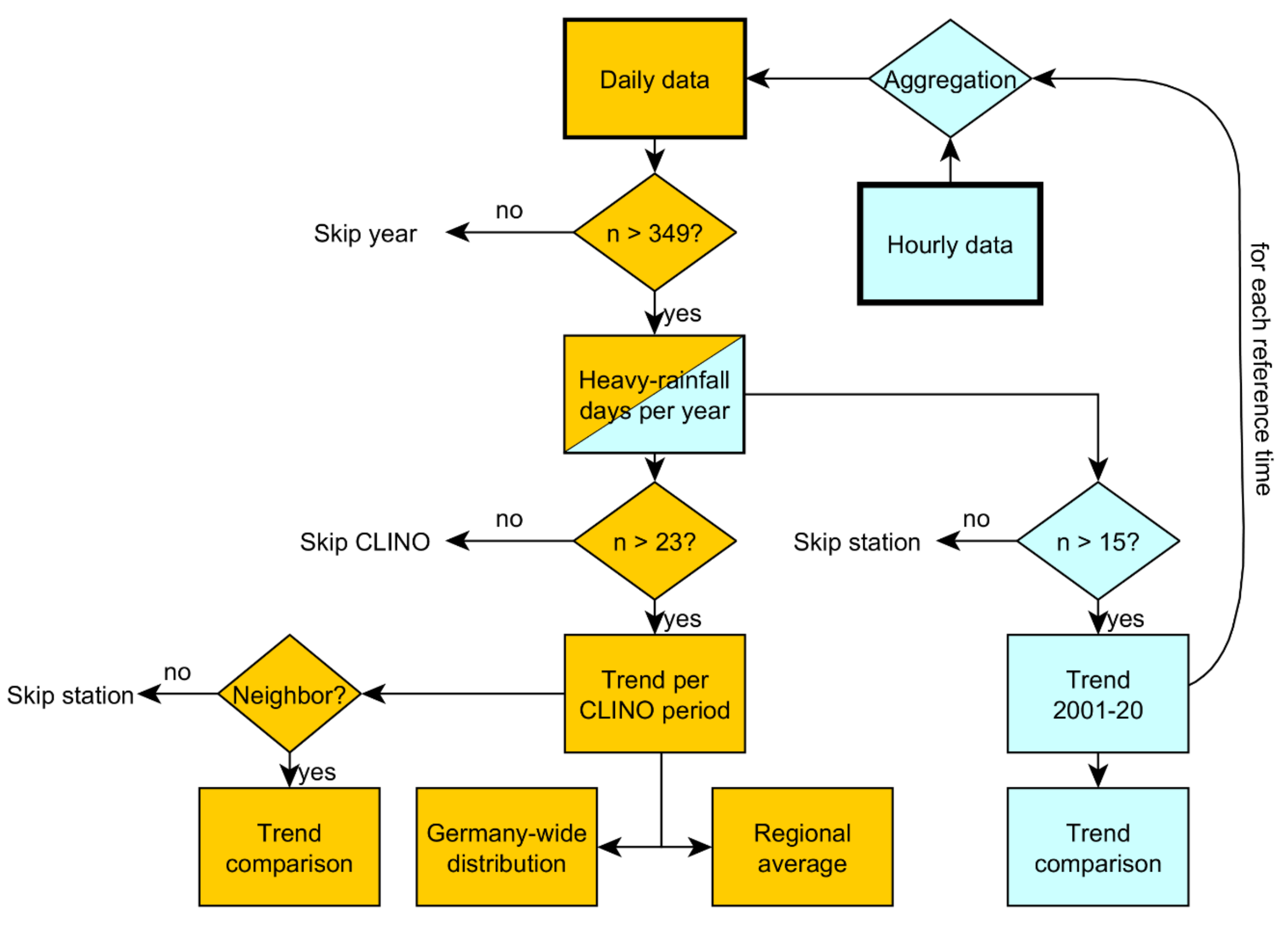
2.1. Multi-Decadal Trend Analyses of Heavy Rainfall Days

Multi-decadal data on daily precipitation was available from the DWD [27]. The DWD hosts 5930 historical datasets (i.e., until the end of 2018) and 1994 recent datasets (July 2018 until December 2019) of RR (precipitation) stations. For each station and year, we counted heavy rainfall days, alternatively defined as days with ≥10 mm, ≥20 mm, and ≥30 mm rainfall. To account for small data gaps, only years with less than 16 missing or negative values were considered (cf. Figure A1 in Appendix A).
The period 1901–2019 was sub-divided into ten periods of 30 years. These overlapping periods are shifted by 10 years. They correspond to those used for calculating Climate (Standard) Normals [28] (CLINO, henceforth, “CLINO” refers to our periods). The last complete CLINO period ranges from 1981 to 2010. It was amended by the current one that misses the year 2020.
The trend strength and direction was determined for each station and CLINO period using the non-parametric Mann–Kendall trend test as implemented in the rkt library for the R software package [29]. For a time series of n elements, here, 30 annual values of heavy rainfall days, Kendall’s tau (τ) is the number of positive differences minus the number of negative differences between pairs of values aj and ai with i < j divided by all possible pairs:
τ = i = 1 n 1 j = i + 1 n sgn a j a i 1 2 n n 1
where the function sgn gives −1 for negative and +1 for positive differences. Accordingly, τ ranges from −1 for a monotonic negative trend to +1 for a monotonic positive trend. Trends were calculated if at least 24 years were available (cf. [28]). Apart from the annual trends, we also assessed the trends for the winter (November–April) and summer half-years (May–October).
Trends could be calculated for in total 4663 stations. The availability changed with the CLINO period. We focused on the second half of the 20th century when the numbers were highest (Figure 1b). The time period after World War II was also in line with previous trend analyses of heavy rainfall for Germany (e.g., [23,30]).

2.2. Uncertainty Assessments

2.2.1. Different Operating Periods

The complete but potentially biased dataset was compared to the 111 stations with no (n = 66) or one missing trend value (n = 45) during the 10 overlapping CLINO periods since 1901 (Figure 1a, Table A1 in Appendix A). We assumed that similar trend distributions during the last five CLINO periods indicate that the consistent assessment over more than 100 years is representative for the whole of Germany.
For some combinations of threshold and CLINO period, the distribution of Kendall’s tau differed significantly from the normal distribution, according to the Shapiro–Wilk test. Therefore, we applied the non-parametric Mann–Whitney test to all 30 combinations of thresholds and CLINO periods in order to test whether the distributions of these 111 stations differ significantly (p < 0.05) from the other stations.

2.2.2. Location Shifts

Each dataset was accompanied by metadata on changes in time, location, and instrumentation. The location of stations was reported as longitude and latitude. To compute the great circle difference between pairs of locations (of a shifted station and of neighboring stations), we used the R package sf. [31]. As expected, older stations (with more valid trend values) were more often shifted than younger stations (Table 1). Nonetheless, 20% of the 111 stations with 9–10 trend values still remained at their original location, compared to 54% of the other stations. Similar to the above, we applied the Mann–Whitney test to compare the trend distributions of stable and shifted stations for all thresholds and CLINO periods (n = 30).
To assess the local effect of location shifts more specifically, we additionally selected for each CLINO period the stations with valid trend values. However, to reduce the impact of location shifts on the computed trend value, we only considered stations located for at least 24 years at the same position in a given CLINO period. The closest neighboring station was joined to each station, with double entries being removed (A joined to B and B joined to A).
As the average location shift was smaller than the average difference to neighboring stations (>11,000 m), we chose a threshold of 2500 m, which allowed us to select enough stations with elevations differing by less than 100 m while still being close to the average (unweighted) difference between past and current (or final) locations (1700 m). For these 45 pairs, the paired Wilcoxon signed-rank test was used after the Shapiro–Wilk test, showing that the distribution of tau differences was not normally distributed for the threshold of 30 mm d−1.

2.2.3. Changed Reference Time for Daily Sums

Unlike location shifts, the reference time for daily sums was changed for almost all current stations, i.e., with time-series starting in 1981 or before. The metadata revealed that daily sums were increasingly measured between 5:51–5:50 UTC since 2001 but between 7:30–7:30 UTC (until 2012) and 7:00–7:00 UTC (former GDR, until 1990) before. To assess how the reference time affects trend analyses, we calculated alternative daily sums for stations with hourly data from the DWD [32] starting from 6:00, 7:00, or 8:00 UTC; additionally, we included 0:00. Heavy rainfall days were counted annually using the same thresholds as for the daily data, considering only days without missing data. Likewise, years with more than 15 missing days were discarded from the trend analyses.
All time-series of hourly data were too short for matching the criteria for valid CLINO trends (cf. Section 2.1) as the longest time-series had only 22 values in the period 1991–2020. So, we calculated Kendall’s tau for the period 2001–2019 and allowed for four missing years. In this way, we conducted a two-factor ANOVA with an ensemble of 86 stations to evaluate simultaneously whether the effects of the independent variables “threshold” and “hour” on Kendall’s tau are significant (p < 0.05), after the Shapiro–Wilk test confirmed the normality of the residuals.

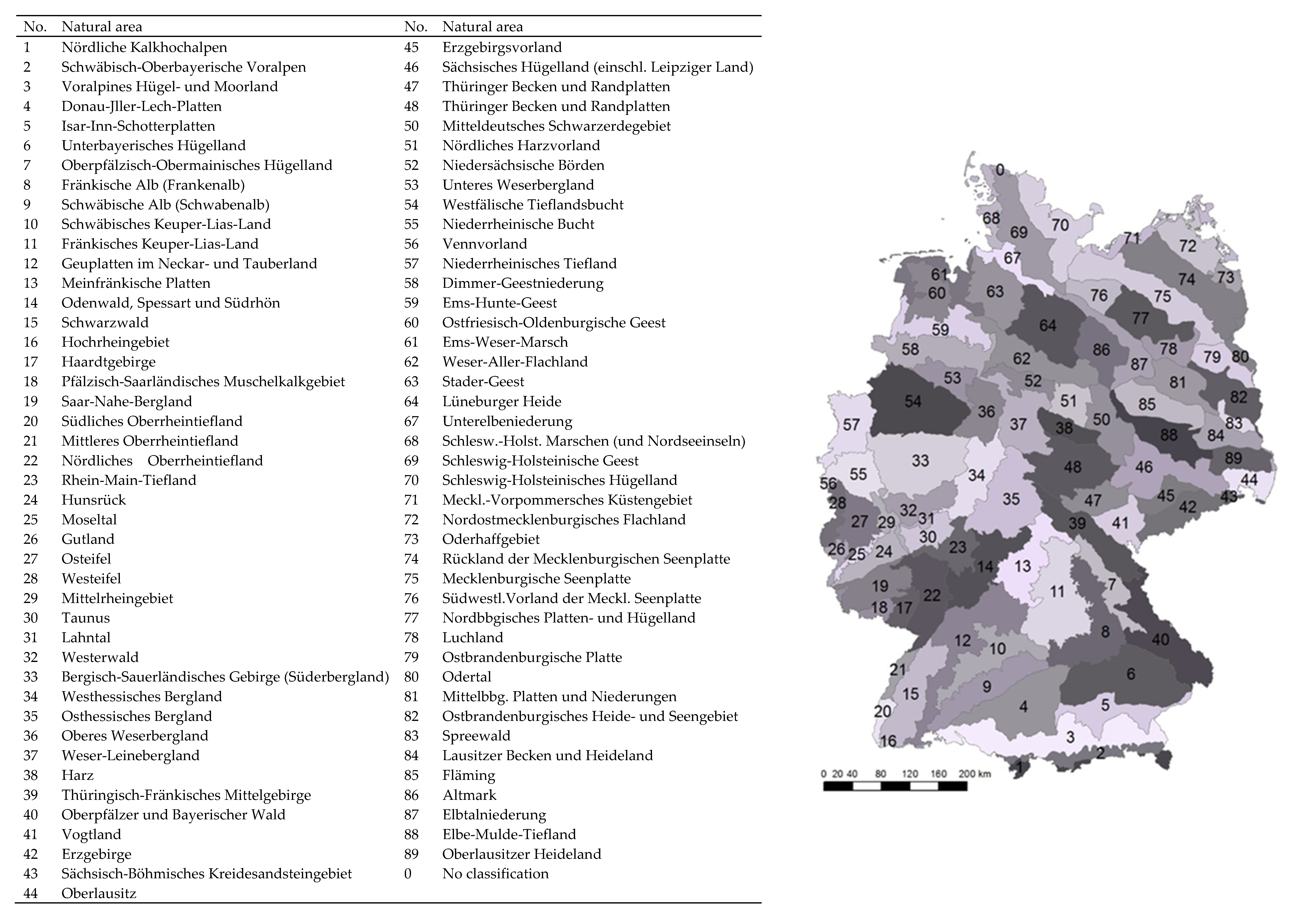
2.3. Regional Trend Pattern

We assigned the stations to the second aggregation level of the German natural regions (“Naturräume”, [33], Figure A2 in Appendix B). In order to have sufficient trend values for all 87 regions, we selected again the years 1951–2019 (Figure 1b). For each region and CLINO period, the average of Kendall’s tau was calculated (cf. [19]), and the dominant trend direction (±) was assigned to identify regions with continuously positive or negative seasonal (winter, summer) and annual trends.
We discussed the 20-mm trends for three of the 111 stations with continuous trend values as examples in more detail. The lowland station Lindenberg (98 m above sea level, a.s.l.) is located in NE Germany. The mountainous station Hohenpeißenberg (977 m a.s.l.) and the Alpine station Zugspitze (2964 m a.s.l.) are located in southern Germany. Hohenpeißenberg has the longest time series in Germany since 1781—a unique time series over almost 240 years. These stations were slightly shifted in the past, by below 135 m except Hohenpeißenberg in 1940 (273 m). To fill the “elevation gap” between the two latter stations, we included the nearby Wendelstein station (1832 m a.s.l.), for which data was available from 1951 to 2012. However, its elevation changed by 97 m in March 1963.

2.4. Rainfall Intensity

To provide a preliminary assessment of long-term changes in rainfall intensity, we used data from an own ombrometer (ZALF) with 1–10 minutes resolution located in Müncheberg (52.517494° N, 14.123103° E) in NE Germany starting in 1955 (Figure 1a). The analog data before 1991 had to be digitized.
As an indicator of rainfall intensity, we calculated the rainfall erosivity EI30 for rainfall events according to the German norm DIN 19708, a German adaptation of the Universal Soil Loss Equation (USLE, [34], Equations (2) and (3)). Rainfall events were separated by at least six hours without rainfall. EI30 (in N h−1) is the product of the rainfall energy (E, in J m−2) and the maximum 30-min intensity (I30, in mm h−1):
EI30 = I30 ΣEi,
For each time step i, the rainfall energy was calculated from the rainfall amount (P, in mm) and intensity (I, in mm h−1) according to
Ei = (11.89 + 8.73 log Ii) Pi, if Ii ≥ 0.05 mm h−1
Ei = 0, if Ii < 0.05 mm h−1, or
Ei = 28.33 Pi, if Ii > 76.2 mm h−1
To visualize the time-series for individual stations, we used the Simple Moving Average (SMA),
SMA = i = m n a i n m + 1
where ai is the value for the ith year in the time series. For the number of heavy rainfall days, we used periods of 30 years (i.e., moving CLINO periods, n = m + 29) and of 5 years for visual comparison (n = m + 4). For the erosivity (EI30), the starting year was fixed (m = 1) to show the long-term average as used in the USLE/DIN 19708.

3. Results

Since 1951, the number of heavy rainfall days per year for the whole of Germany has hardly changed, almost independently of their definition (Figure 2a). Except for the CLINO period 1971–2000, the positive and negative trends were balanced. The 111 stations with at least nine trend values represented visually well the overall pattern of Kendall’s tau for 1951–2019 (Figure 2b). This similarity was supported by the statistical analyses (next section).
The recent annual increase of heavy rainfall days between 1971 and 2000 was the result of their increase in summer and partly in winter. Again, there was no clear Germany-wide trend as Kendall’s tau fluctuated around zero, and dominantly positive trends in one CLINO period were compensated by more negative trends in other CLINO periods. Over the last seven decades, there had been a slight shift from more negative trends to more positive trends in summer (Figure 3a), and an inverse shift in winter (Figure 3b), resulting in the almost balanced annual trends. However, the balanced summer trends for the current CLINO period showed that the number of heavy rainfall days did not further increase for the whole of Germany. In general, the trends were more variable for the 10-mm threshold than for the higher thresholds. The comparison of all CLINO periods revealed that the shift in summer almost vanished, resulting in a more balanced trend over the last century, while positive trends dominated in winter.

3.1. Uncertainty Assessments

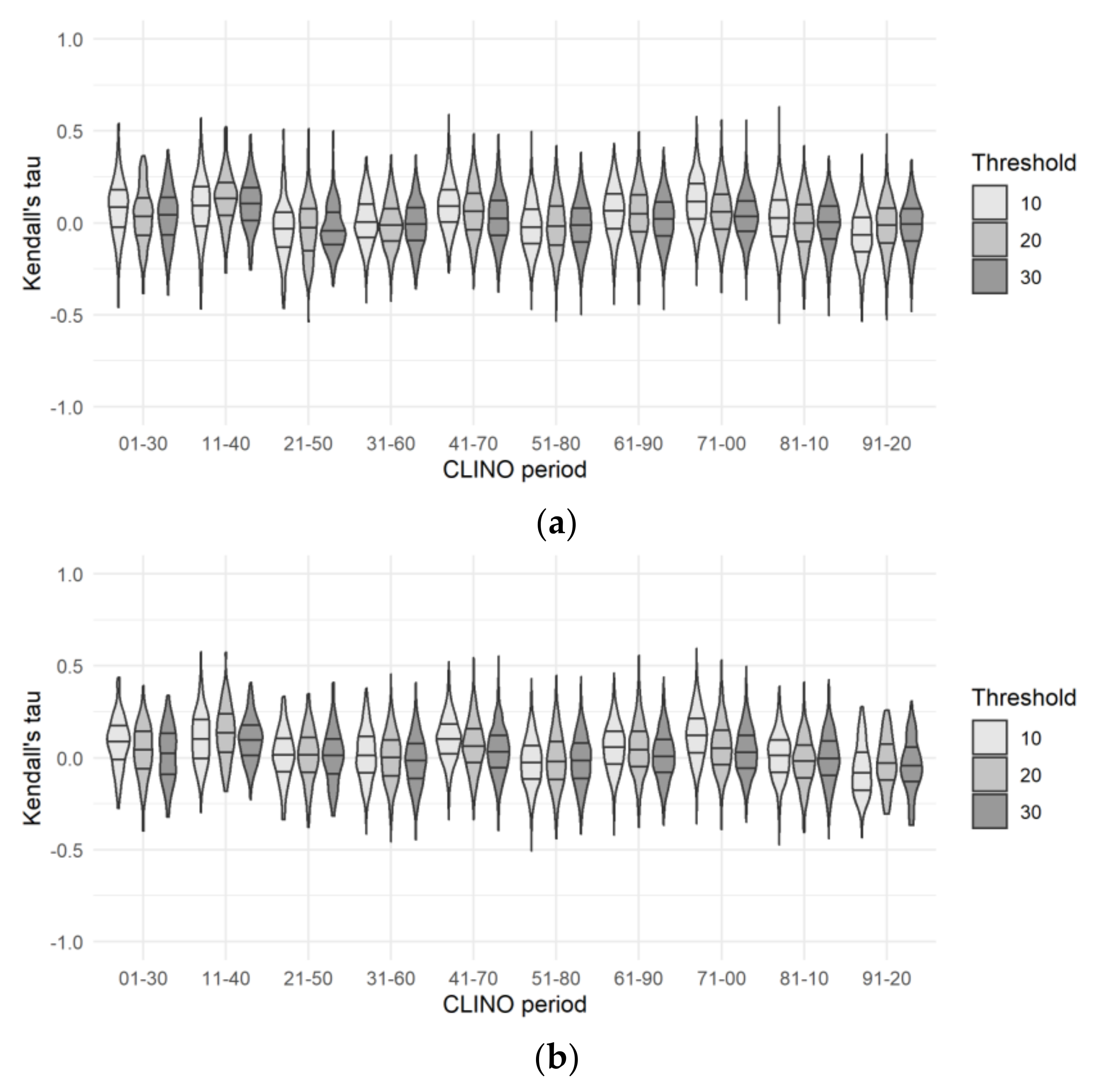
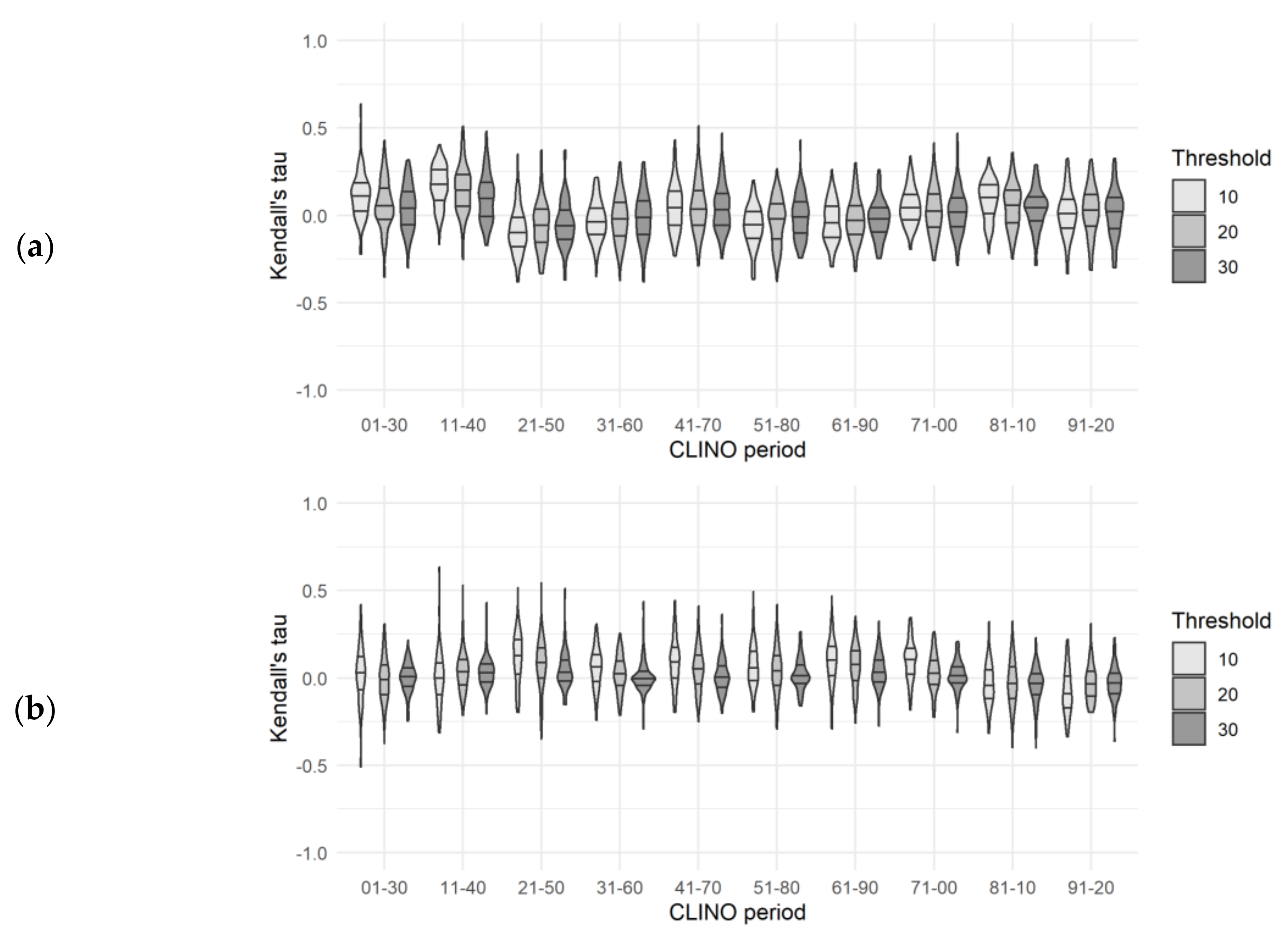
3.1.1. Operating Period

The majority of the Mann–Whitney tests, 24 out of 30, implied only insignificant differences between the stations with continuous trends and other stations. The few significant cases could also be explained by the unequal spatial distribution of these 111 stations (cf. Figure 1a) because only the differences for 20 mm d−1 and 30 mm d−1 between 1961 and 1990 remained significant if only nearby stations were compared (distance < 10 km, n = 420). This general similarity supported that the pattern for earlier CLINO periods of the 111 stations was representative of Germany. Accordingly, the most positive Germany-wide trends (yearly and summer) occurred between 1911 and 1940 (Figure 2b and Figure 3a), followed by more unclear and negative trends afterward.

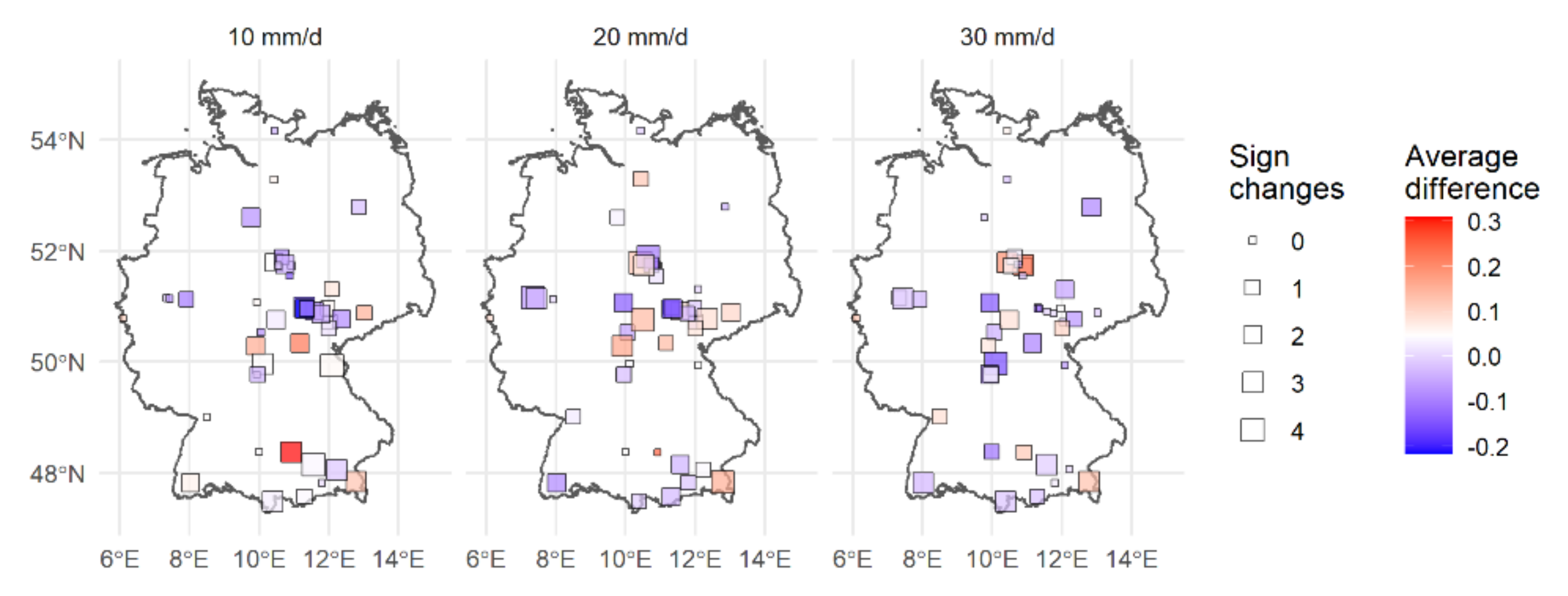
3.1.2. Location Shift

The majority of 30 Mann–Whitney tests showed that the distributions of tau values at shifted and stable stations were similar (Table 2, Figure A3 in Appendix C). Only for the period 1921–1950, significant differences were found for all three thresholds.
The paired tests for nearby stations revealed insignificant differences for all thresholds. For individual stations, however, location shifts could affect both the strength and the direction of trends. The impact was spatially highly variable and lacked a clear pattern (Figure 4).

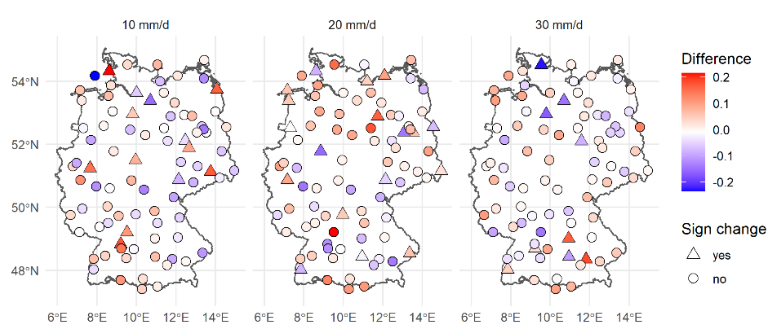
3.1.3. Reference Time

According to the ANOVA, the reference time for daily sums did not significantly affect Kendall’s tau, in contrast to the threshold for heavy rainfall days. Nonetheless, the change in tau varied among the stations. The spatial pattern depended on the threshold for heavy rainfall. Opposing trend changes could occur over short distances (Figure 5). With 6:00 UTC as a reference, the trend direction changed for 12–27% of the stations. The share was proportional to the time shift, ranging on average from 13% for 7:00 UTC to 24% for 0:00 UTC.

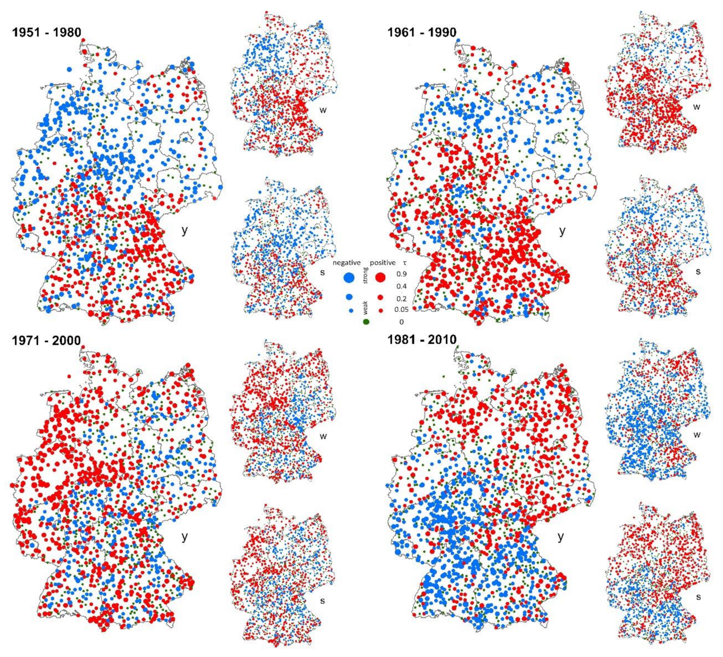
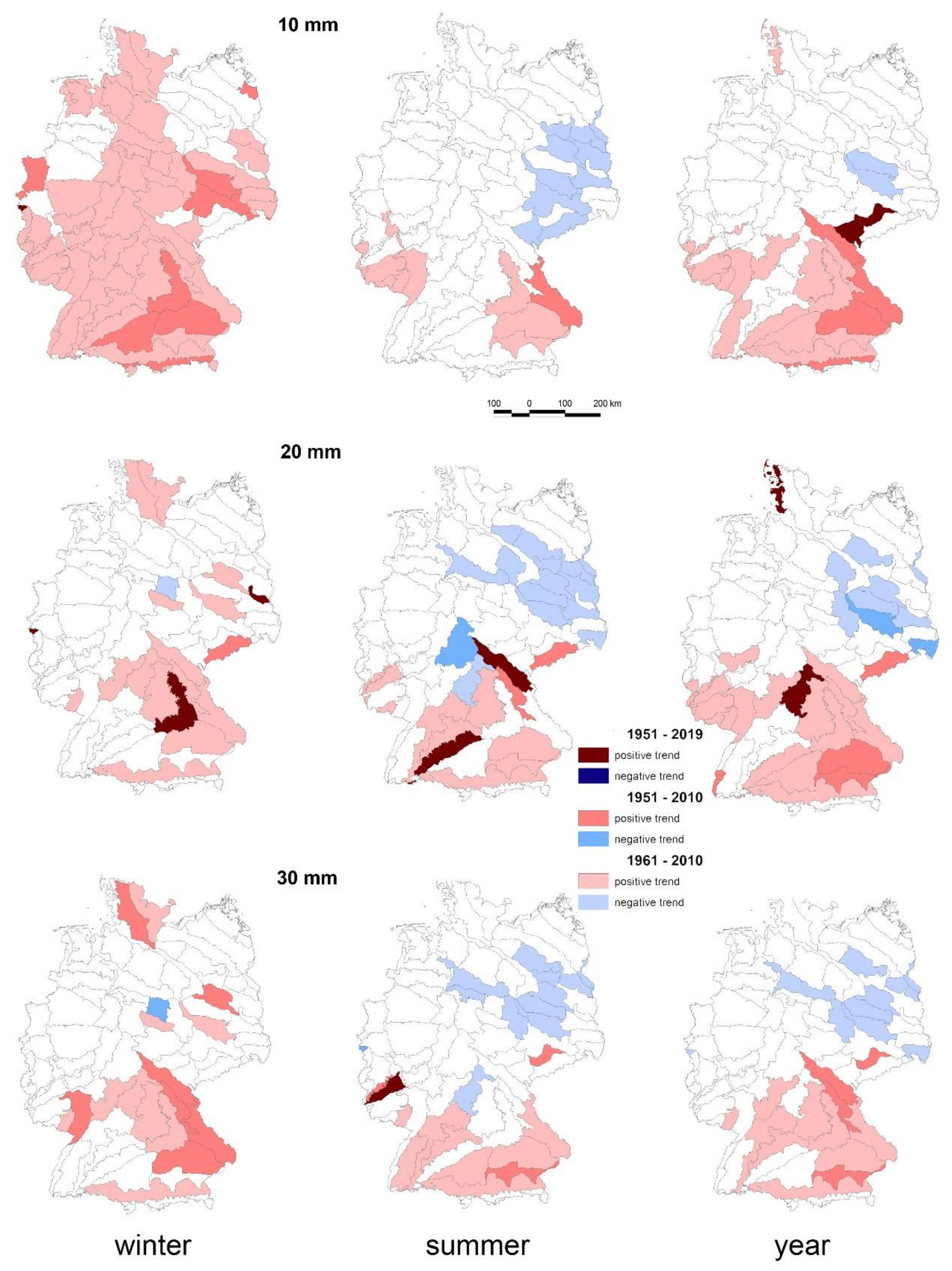
3.2. Regional Trend Pattern

Despite the high local variability of trends in each CLINO period (Figure 6), distinct spatial trend patterns became more evident if station data was aggregated by the natural regions (Figure 7). Only a few natural regions had continuously positive trends since 1951, and none with negative trends (dark colors). Regions with dominantly positive trends during the last CLINO periods were mainly located in the foothills and mountainous areas in southern Germany. Predominantly negative trends were observed in Central Germany. The spatial patterns of trends during summer months resembled those of the annual trends. While winter trends were also positive in southern Germany and the coastal region of Schleswig-Holstein, regions with dominantly negative trends were not relevant.
The choice of the threshold value partly influenced the regional pattern. Since 1961, there had been a general Germany-wide increase of days with rain intensities ≥10 mm d−1 in winter, except for some regions in North-West (NW) and NE Germany. With values of 20 and 30 mm d−1 as a threshold, the increase between 1951 and 2010 was restricted to regions in southern Germany and some regions in Central Germany. The effect of the choice of the threshold value was smaller for the summer period and for the annual trend.

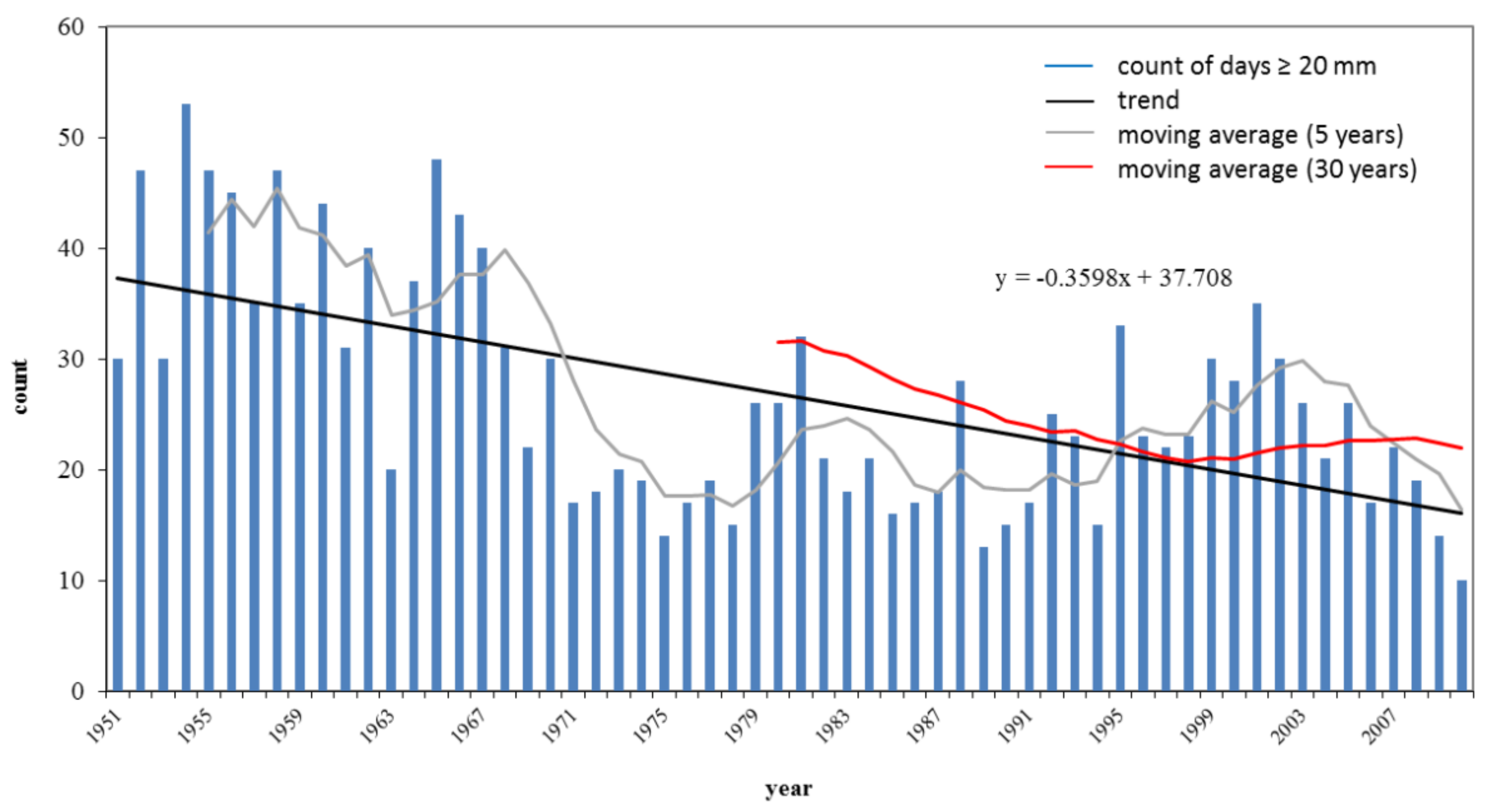
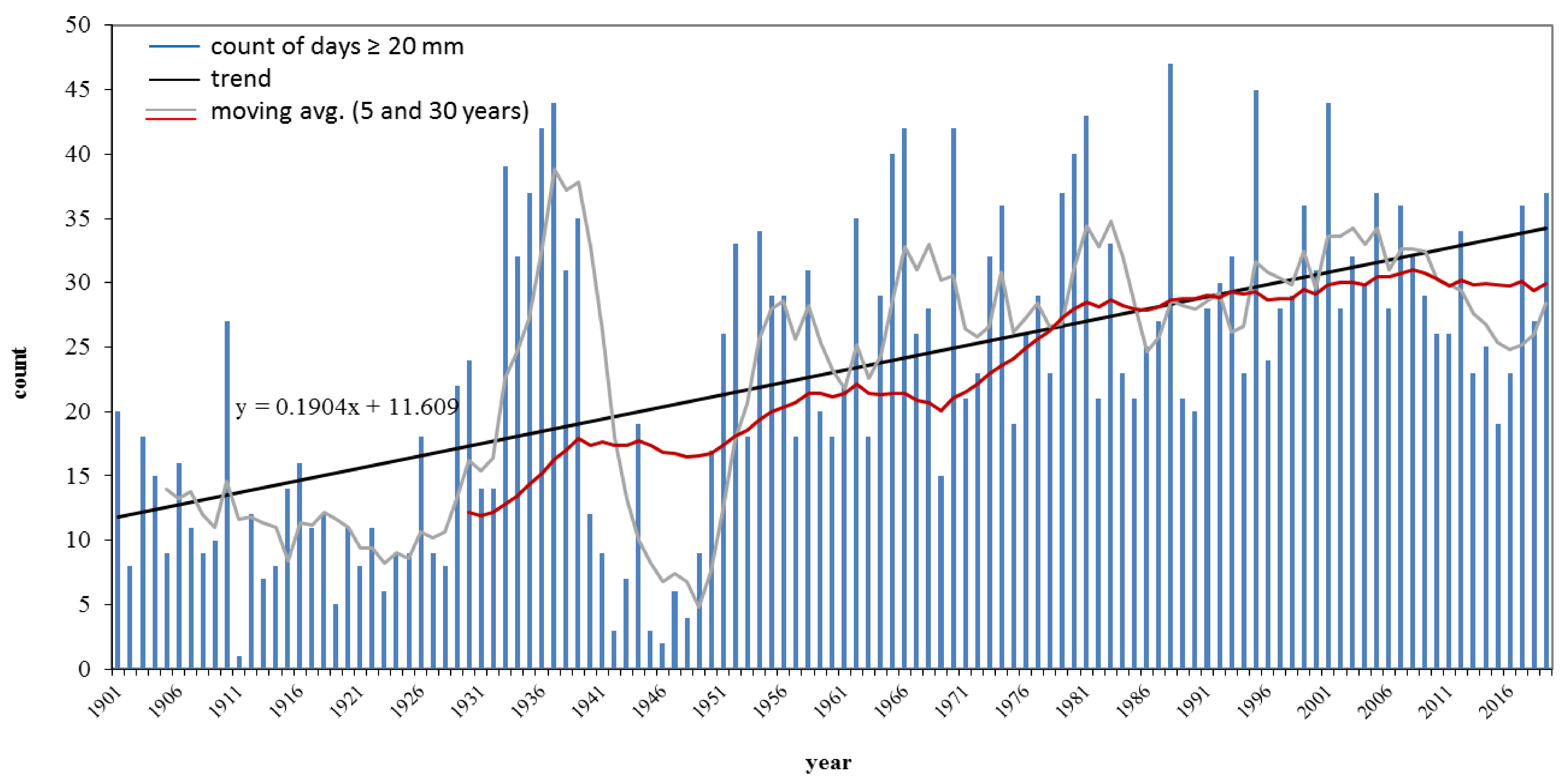
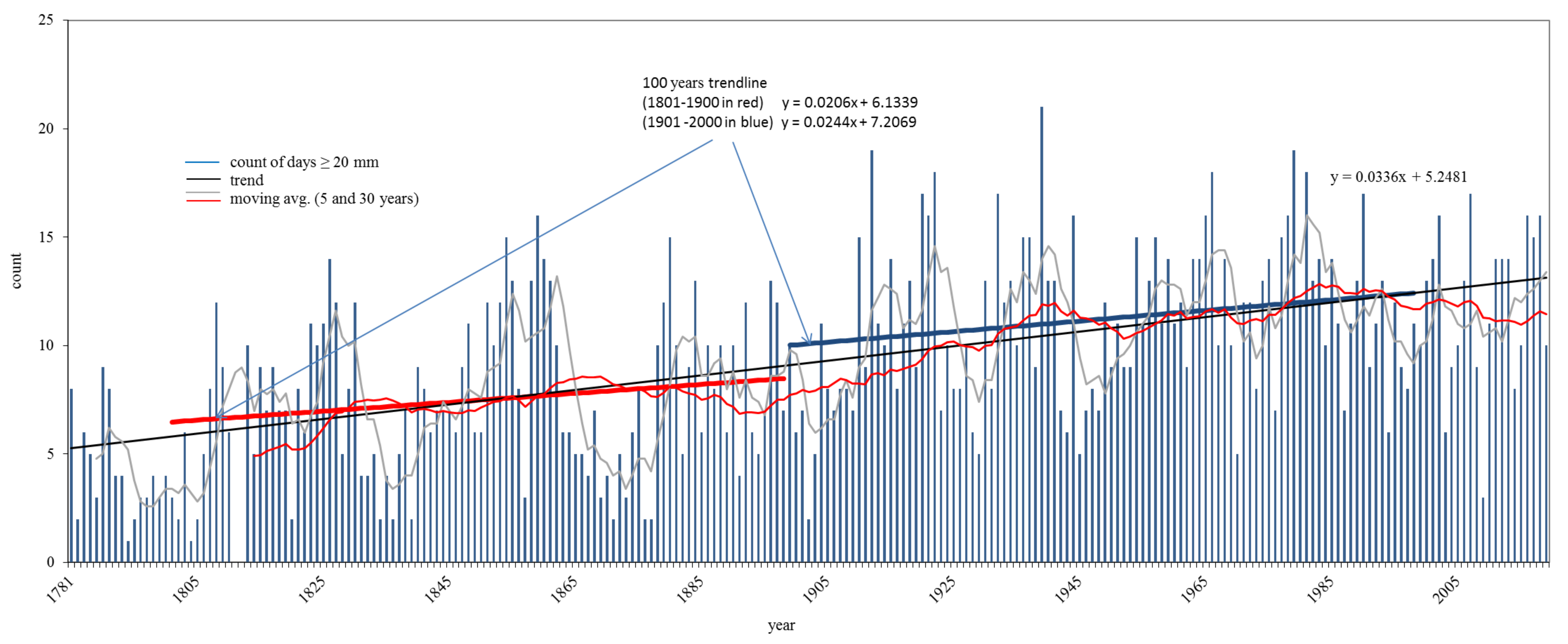
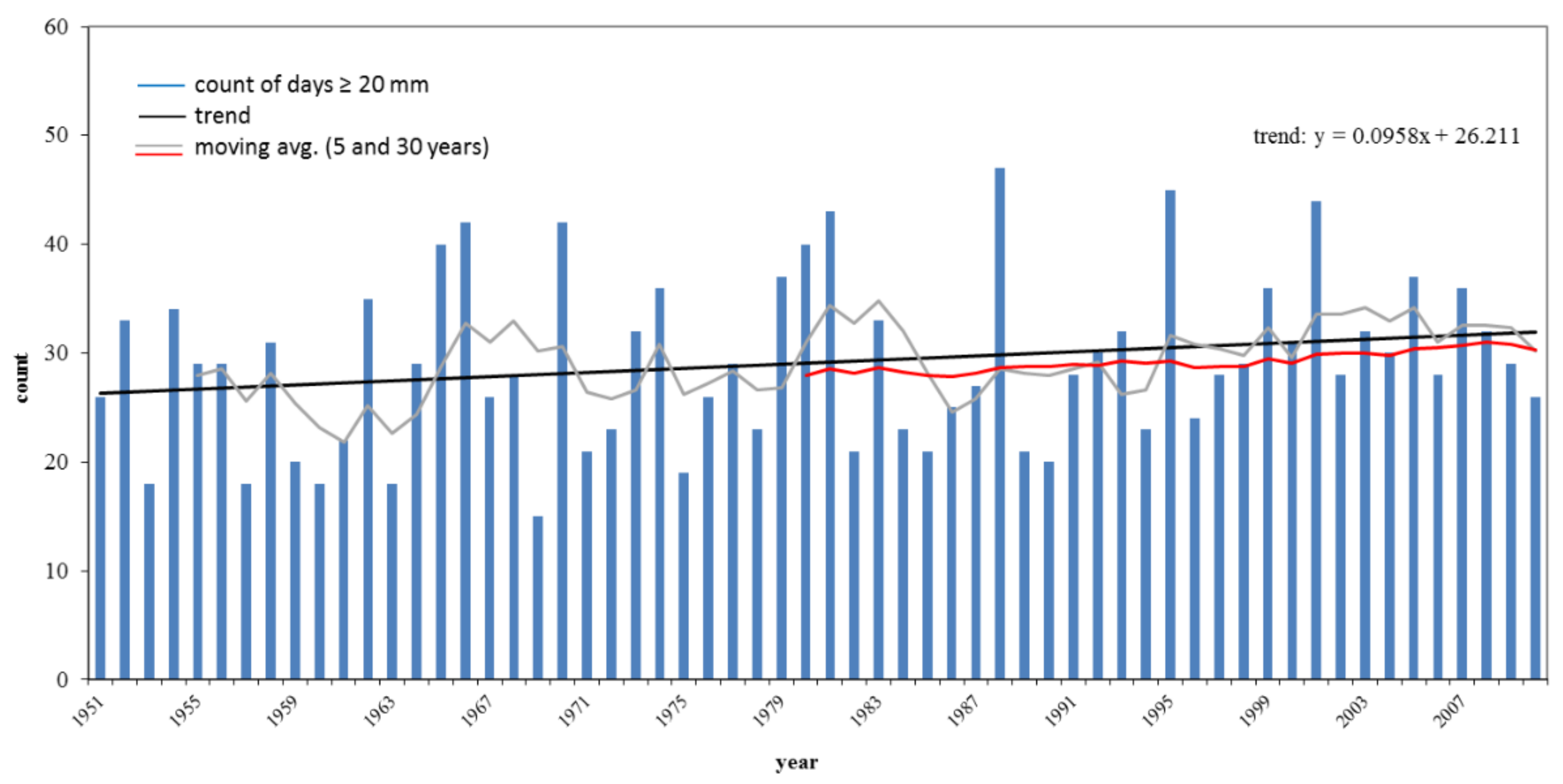
3.3. Long-Term Trends for Selected Stations (20-mm Threshold)

The selected stations exemplified the Germany-wide variation in space and time, including opposing trend directions. There was both temporal and spatial variability as well as fluctuations on different time scales. The annual number of heavy rainfall days in Germany ranged from around 0–10 in the lowlands (e.g., Lindenberg, Figure 8) to around 20–40 days yr−1 in the Alps (e.g., Wendelstein and Zugspitze, Figure 9 and Figure 10). While the number of heavy rainfall days decreased significantly from around 40 to currently 20 days during the last 60 years at Wendelstein (Figure 9), the number at Zugspitze increased, albeit slightly (Figure 11). However, the frequency of heavy rainfall days doubled at the latter station since the beginning of the 20th century. A similar increase occurred at Hohenpeißenberg, but already during the 19th century (from 5 to 10 days). The average of 7.5 days further increased to 11.2 days in the 20th century. The increase in the frequency of heavy rainfall days was steepest between 1890 and 1940. Since then, the trends oscillated, so the frequency remained almost stable during the last 70 years (Figure 12).
The few station changes were unrelated to these trends. For instance, the relevant downward trend at Wendelstein started after the elevation change in 1963. Likewise, the trend changes at Hohenpeißenberg appeared before the two location shifts between 1940 and 1948.
Compared to the stations in the mountainous south, Lindenberg showed a very weak positive trend during the last century with fluctuating trends over 30 years. The increase since 1951 differed from the negative regional trend in other parts of NE Germany.

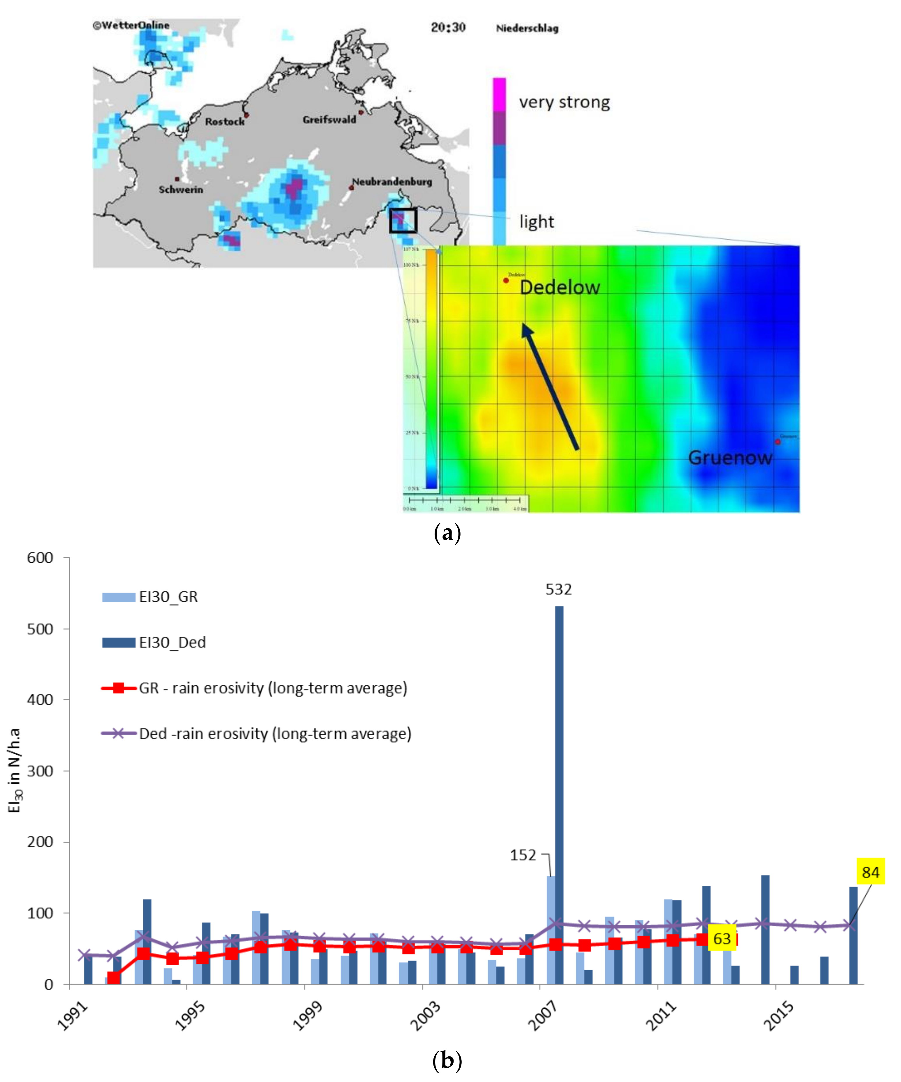
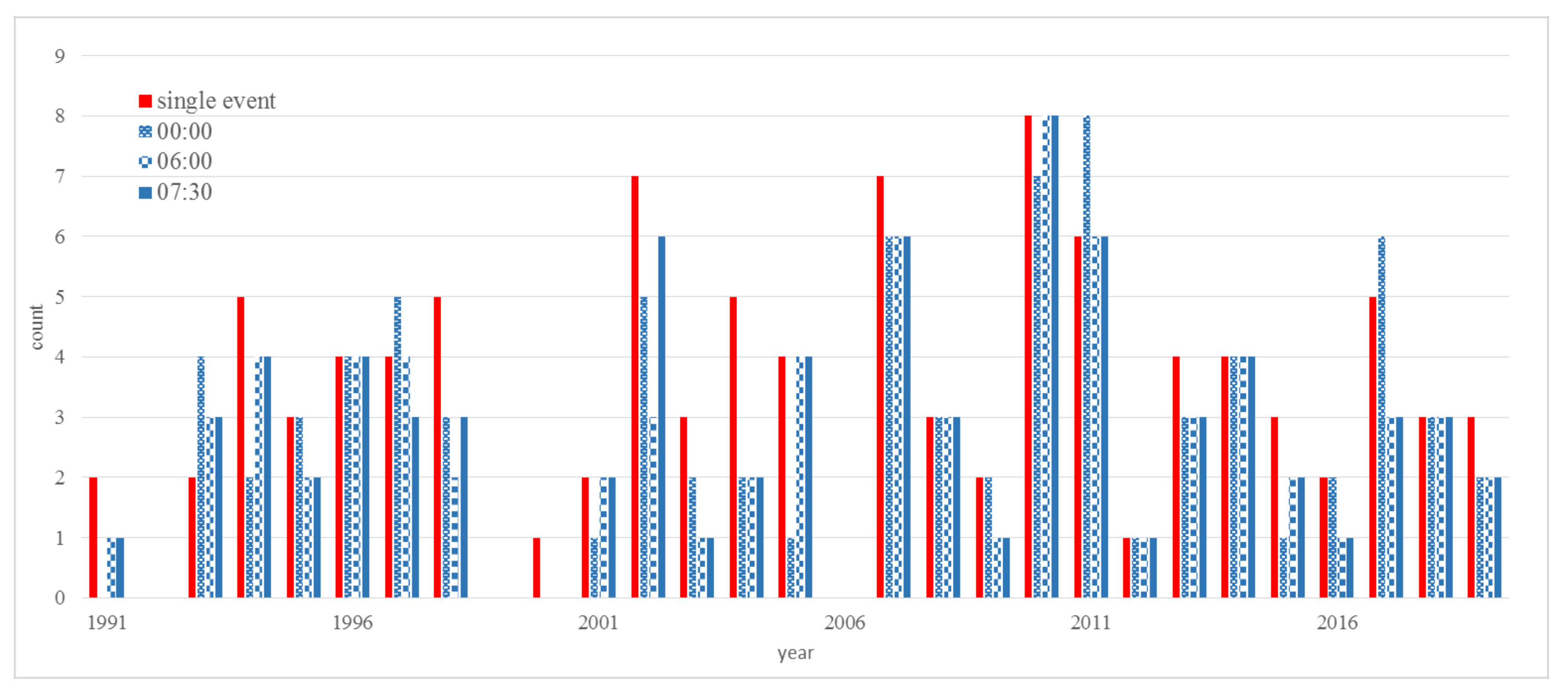
3.4. Temporal Variability of Rainfall Erosivity—The Case Study Müncheberg

Similar to the nearby station in Lindenberg (distance 33 km, Figure 8), the number of heavy rainfall events changed hardly during the recent CLINO period (Figure 13). Aggregating the high-resolution data to rainfall events instead of daily sums had no influence on the trend. The absolute deviations were small compared to the inter-annual variability. The number of heavy rainfall events was, on average, 0.6 higher than the number of heavy rainfall days.
In contrast to the negligible trend in heavy rainfall days—independent of the reference time—(Figure 13), the magnitude of rainfall events increased more significantly (Figure 14). The long-term average of EI30 changed from 45 N h−1 (the mid-1970s) to 65 N h−1 (2019). The strongest change occurred after 1990 (red trend line) with an average value of 80 N h−1 for the last 30 years. The annual values generally ranged widely, from about 11 to >300 N h−1. However, the three highest values happened after 2000.

4. Discussion

4.1. Spatial and Temporal Trend Patterns

After 1951, the multi-decadal trends of heavy rainfall days in Germany revealed:
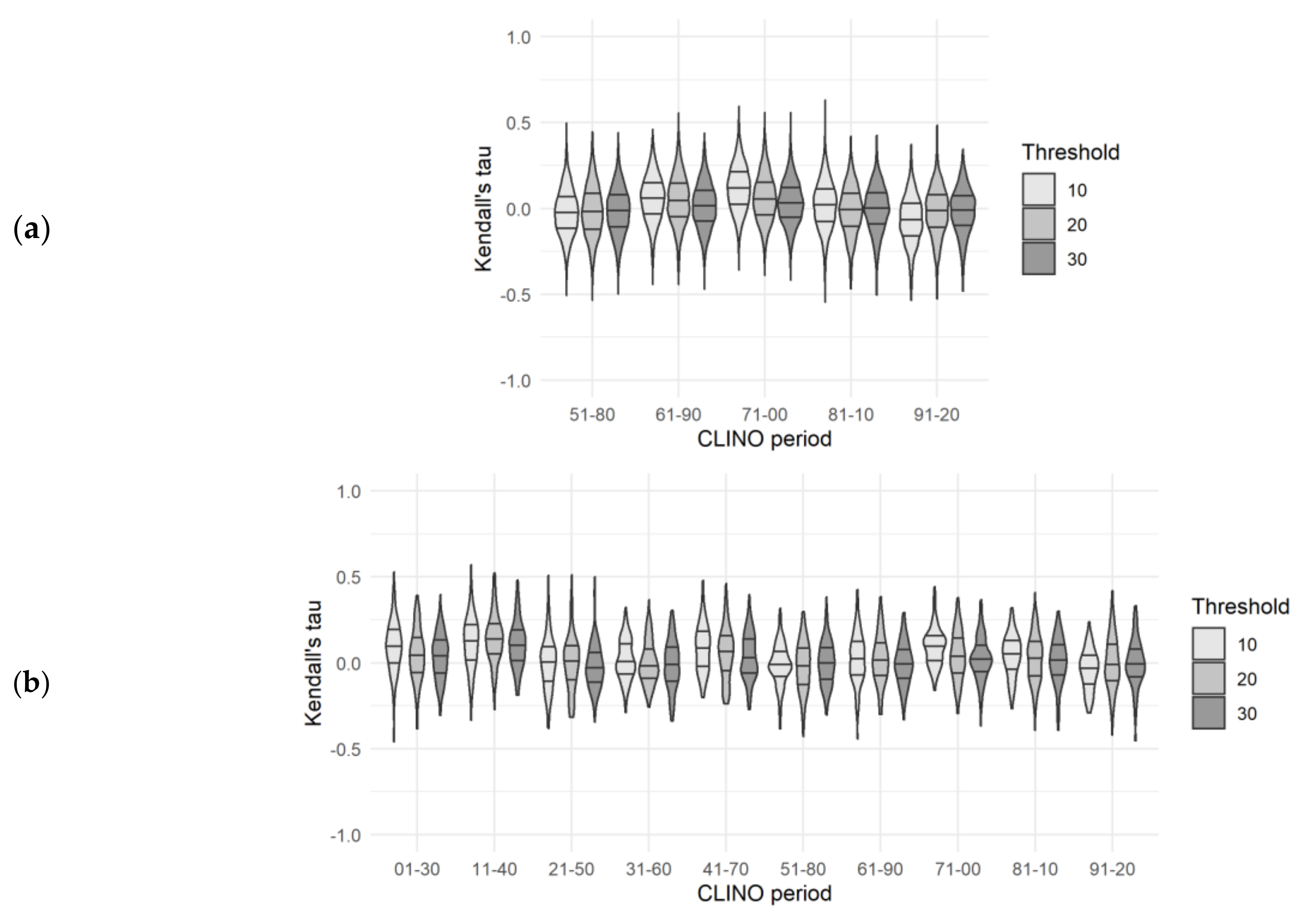
  • The annual frequency of heavy rainfall days changed a little. Positive trends dominated for the 30 years between 1971 and 2000, which corresponded to an increase in summer and partly in winter. During the remaining CLINO periods, the variation of Kendall’s tau around zero was the result of opposed trends in both seasons.
  • There was a weak increase in summer days, while winter days decreased. However, taking also the first half of the 20th century into consideration, these changes were within the range of previous CLINO periods.
  • Most of them showed continuously positive winter trends, which corresponded to more winter precipitation, as observed by Pauling and Paeth [35]. However, the most recent data revealed balanced, even slightly negative trends.
  • Despite significant differences in Kendall’s tau, the alternative thresholds of 10, 20, and 30 mm d−1 gave consistent results. The trends were more variable for the 10-mm threshold than for higher thresholds.
Recent trend studies for Germany typically started with the year 1951, e.g., [36,37,38]. However, even 6–7 decades were relatively short to detect and evaluate long-term trend changes. The assessment of previous CLINO periods showed that trend directions changed repeatedly throughout Germany. The strongest positive Germany-wide trends during the last 120 years occurred at the beginning (1901–1940) and in the middle of the 20th century (1941–1970). In comparison, the positive trend at the end of the century (1971–2000) was rather weak (Figure 2 and Figure 3).
For individual stations, with time-series up to 1781, important changes also occurred previously. This was similarly shown for winter and extreme precipitations [35,39]. In southern Germany, for instance, the heavy rainfall days at Zugspitze became more frequent during the 20th century, but at Hohenpeißenberg, already during the 19th century, followed by oscillating trends. All these examples underlined the importance of long-term monitoring stations.
However, these trends and trend changes were highly variable in space with opposing trends within Germany. Nonetheless, regions with stable trends could be identified—independent of their orographic setting. Long-term trends increased, especially in the south-eastern foothills and mountainous areas but also in Northern Germany, close to Denmark. In contrast, Central Germany experienced dominantly negative trends. The latter outcome agreed with previous findings that extreme events would be less probable in East Germany [39]. For the Saxon-Polish border area, Łupikasza et al. [12] also reported spatial variations in trend directions for 1951–2006. For the German part, their reported positive trends in extreme precipitation in all seasons were partly in line with our findings.

4.2. Reliability of Long-Term Trend Analyses

However, the use of long-term data raised the question of data inconsistency and uncertainty in trends. Rejecting inconsistent data consequently was no option for multi-decadal trend analyses in Germany because all stations were affected by changes. This was especially true for older stations. Nonetheless, our assessments showed that data inconsistencies not necessarily affected regional and national trend analyses—unlike the choice of the threshold for heavy rainfall days.
All daily values refer nowadays to a reference time, which is different from previous decades. This change could indeed affect the strength and direction of trends. However, the overall impact was found to be small. This could be explained by the typical occurrence of heavy rainfalls in the afternoon [40]. Additionally, the location of almost half of the stations changed, often several times in the past. Compared to the distances between rainfall stations, these location shifts were normally small. Although the rainfall intensity and erosivity could be highly variable for single events at the sub-kilometer scale [41], the comparisons of nearby stations as well as of stable and shifted stations in Germany indirectly confirmed that the distribution of trends was also not significantly affected. Nonetheless, the outcomes of statistical tests differed highly in space and partly for the thresholds as well as CLINO periods. Although inconsistencies in the existing data increased with the station age, i.e., length of data records, the selected 111 stations with almost continuous trends since 1901 represented well the general pattern of Germany-wide trends. Nonetheless, regional studies should further explore the validity and transferability of our findings—especially in regions with scarce long-term data.
Albeit being small for national and regional trends, data inconsistencies could have more important consequences for trend analyses for single stations. Specific knowledge and more detailed data were needed to assess how reliable individual trends were, especially where combined data inconsistencies were relevant—both aspects were outside the scope of this study. Although the metadata proved to be useful to assess the reliability of trends, another source of uncertainty arose from missing information, especially for early periods. The currently available metadata began more than 10 years after the data records of 32% of the 4663 stations with calculated trends (n = 1475).

4.3. Rainfall Intensity and Erosivity

Since the beginning of the 20th century, precipitation increased globally by about 1%, particularly in the middle and higher latitudes of the northern hemisphere [42]. For western Germany, Neuhaus et al. [43] even found a 2% increase in precipitation per decade between 1937 and 2007. Such a rise of the total precipitation without similarly more heavy rainfall days allowed for two conclusions: more precipitation below (our) critical thresholds or more intense heavy rainfall events.
While assessing the weather situation during the Elbe flood in 2002, Rudolf referred to the physics of heavy precipitation [42,44]. The stronger dynamics are linked to the water cycle and energy turnover in the atmosphere, both of which have been intensified due to global warming [45,46,47]. On moist land surface, higher temperatures result in more evaporation. This can lead to more dehydration of the soil, while the evaporated water contributes to (more) precipitation elsewhere. All this leads to increasing lability of the atmospheric stratification and an increase in extreme events, such as storms and heavy precipitation [31,47].
The above-mentioned thermodynamic effect has led to an altered precipitation regime during the last few decades, as also observed by ombrometers at stations or using current rain radar products [48]. Indeed, the case study of Müncheberg (Figure 14) revealed years of high rain erosivity occurring frequently since 1955, but more often during the last 30 years. The nearly doubled average erosivity for the last three decades compared to the decades before (1961–1990) is in line with conclusions recently derived from shorter time-series from other stations in this region [48]. The rainfall erosivity has also increased in western Germany—already since the mid-1970s, after the variable trend directions since 1937 [22]. The increase of the magnitude of erosive events was even indirectly deduced for the whole of Germany [25,49] and Europe [3,38,39,50], however, with seasonal and regional differences (e.g., [19]). Climate scenarios suggest a further increase in rainfall erosivity and seasonal shifts of rainfall (e.g., [48,51,52]), resulting in higher soil-erosion risk. Nonetheless, many questions remain unanswered to unambiguously attribute the contribution of anthropogenic climate change to the risk of extreme weather and climate events as well as their prediction [53].
In order to better assess the actual and potential erosion risks, more recent and historical data is urgently needed [54], as even 60 years of data cannot comprehensively represent changes in precipitation. Firstly, the nationwide rain radar in Germany enables more comprehensive evaluations of precipitation, in particular heavy rainfall. It has already allowed identifying more than 11,000 heavy rainfall events since 2001 all over Germany [6]. These events occur at any place in Germany at any time, especially between May and October. The high spatial variability of extreme rainfall erosivity (e.g., [40,41]) is exemplified by the stations of Grünow and Dedelow, 95 km north of Müncheberg. In 10.6 km distance, the erosivity in 2007 changes from 152 to 530 N h−1—due to the extreme event on 5 June 2007 when a thunderstorm hit Dedelow but missed Grünow (Figure 15a). Such extreme events even influence long-term average annual sums of EI30 (Figure 15b). The difference of 33% between Dedelow (84 N h−1 a−1) and Grünow (63 N h−1 a−1) is, e.g., close to the 50% of an isolated extreme event in Berlin-Tegel [48].
Secondly, as shown for Müncheberg, long time-series may not be readily available. Therefore, the DWD started digitizing historical ombrograph data as a “national treasure” to make new high- resolution data available for future research [54,55]. Similar efforts are also being undertaken in other countries [56]. In the absence of measurements, newspapers, statistical yearbooks, or church books can give a vague idea of the occurrence and frequency of certain precipitation extremes. In NE Germany, near the stations, Dedelow and Grünow, heavy thunderstorms of about 18–82 mm occurred within 15 km distance each other between 8 July and 9 July 1857 (Figure 16). Due to the lack of accurate records (e.g., minute or hourly values), daily sums can be determined from such historical data but not the precipitation intensity or erosivity.

5. Conclusions

All digitally available daily and hourly station data from the German Meteorological Service were used to assess whether Germany experienced multi-decadal trends towards more heavy rainfall days during the last decades. Independent of the threshold for heavy rainfall (≥10, ≥20, or ≥30 mm d−1), a general long-term trend was not apparent. It could be concluded that:
  • For the whole of Germany, the trend variability after 1951 was within the range of previous changes.
  • The direction and strength of multi-decadal trends of heavy rainfall days, however, varied in space and time. After 1951, stable positive trends occurred in southern and parts of northern Germany, but stable negative trends in Central Germany.
  • Despite the frequent changes in the location of stations and in the reference time for daily sums, the trends could be considered reliable for regional to national studies. The impact of data inconsistency on the overall trend pattern was smaller than the threshold but varied among individual stations.
  • Although not occurring more frequently, heavy rainfall events became more intense, and the average yearly erosivity was significantly higher during the last 20 years. Our results from NE Germany supported previous findings in other regions.
It is highly recommended to make (more) historical data accessible to better understand current and possible future changes in rainfall patterns. Future research should further explore how data inconsistencies affect trends of (different) rainfall indices in different regions and assess the drivers of trend variability.

Author Contributions

Conceptualization, methodology, software, validation, investigation, D.D. and A.G.; resources, D.D. and A.G.; writing—original draft preparation, D.D. and A.G.; writing—review and editing, D.D. and A.G.; visualization, D.D. and A.G.; project administration, D.D.; funding acquisition, D.D. All authors have read and agreed to the published version of the manuscript.

Funding

D.D. was supported by the German Federal Ministry of Food and Agriculture (BMEL) and the Ministry for Science, Research, and Culture of the State of Brandenburg (MWFK). The project was supported by funds of the Federal Ministry of Food and Agriculture (BMEL) based on a decision of the Parliament of the Federal Republic of Germany via the Federal Office for Agriculture and Food (BLE) under the innovation support programme. A.G. was partially funded by the German “Bundesministerium für Umwelt, Naturschutz und nukleare Sicherheit (Federal Ministry for the Environment, Nature Conservation, and Nuclear Safety)”.

Acknowledgments

We thank the DWD for providing the rainfall data, namely, Mario Hafer and Elmar Weigl (Offenbach) and Falk Böttcher (Leipzig). We are thankful to Dominique Niessner (IGB), Horst H. Gerke (ZALF), and three anonymous reviewers for their helpful comments.

Conflicts of Interest

The authors declare no conflict of interest.

Appendix A

Table A1. Stations with less than two missing trend values for CLINO periods between 1901 and 2019 (cf. Figure 1, last access January 2020).
IDStation Height (m) LatitudeLongitudeNameData Availability
23853.03119.0233Achim-Embsen1901–2019
645551.850612.0482Aken/Elbe
1707651.730913.0546Annaburg
19816451.374511.292Artern
34963047.706311.4139Benediktbeuern
3718254.421513.4379Bergen/Rügen
37627049.898110.0653Bergtheim
49876047.74538.3111Ühlingen-Birkendorf
64759249.958911.9125Brand/Oberpfalz
691453.0458.7979Bremen
722113451.798610.6183Brocken
8806951.77614.3168Cottbus
110734649.85210.499Ebrach
116610551.460112.6692Eilenburg
117697647.96348.2693Eisenbach
123552547.904412.2977Endorf, Bad
1358121350.428312.9535Fichtelberg
15173852.354714.0638Fürstenwalde/Spree
189917049.28589.1662Gundelsheim
211830250.255310.6832Hellingen
229097747.800911.0108Hohenpeißenberg
244415550.925111.583Jena (Sternwarte)
2465153.50839.7376Jork-Moorende
255970547.723310.3348Kempten
267644849.946111.1637Königsfeld, Kreis Bamberg
2908753.21387.4742Leer
292813851.315112.4462Leipzig-Holzhausen
30159852.208514.118Lindenberg
312167749.911312.5276Mähring
31267652.102911.5827Magdeburg
318854950.114111.9712Marktleuthen-Neudorf
327131348.854812.9189Metten
327917351.045212.2989Meuselwitz
32809853.308312.2937Meyenburg
336428650.868110.8211Drei Gleichen-Mühlberg
342462447.668911.2238Murnau
342612751.56614.7008Muskau, Bad
35643553.457111.5687Neustadt-Glewe-Friedrichsmoor
368543149.411410.4331Oberdachstetten
376127649.2079.5176Öhringen
394638650.481912.13Plauen
39878152.381313.0622Potsdam
406440948.692110.8976Rain am Lech
40813052.609212.3628Rathenow
410358248.966213.1425Regen
410634549.138812.1164Regenstauf
42753253.12889.3398Rotenburg (Wümme)
428741549.384810.1732Rothenburg ob der Tauber
438117951.477611.3123Sangerhausen
46255953.642511.3872Schwerin
47457552.96049.793Soltau
49021354.296613.0615Stralsund
50093853.76112.5574Teterow
512764948.00838.8179Tuttlingen
5142153.744414.0697Ueckermünde
538966448.596213.7864Wegscheid
544210951.200211.9154Weißenfels
544450048.309110.2048Weißenhorn-Oberreichenbach
548325551.14987.1867Wermelskirchen
55139252.29027.8687Westerkappeln
55429050.04218.2331Wiesbaden-Biebrich
56436653.186412.4949Wittstock-Rote Mühle
5732854.69288.5271Wrixum/Föhr
5777154.431712.6837Zingst, Ostseeheilbad
5792296447.420910.9847Zugspitze
594168647.675412.4698Reit im Winkl
31771049.119813.1987Bayerisch Eisenstein1901–2010
73337049.251812.311Bruck
892253.82568.7721Cuxhaven-Altenbruch
9991554.113711.9129Doberan, Bad
127445048.666212.1766Ergoldsbach-Kläham
1480853.48187.7274Friedeburg-Wiesedermeer
161020050.89112.0641Gera-Untermhaus
184049050.812713.3425Großhartmannsdorf/Speicher
191515551.35914.8609Hähnichen
20044654.12459.407Hanerau-Hademarschen
22036651.16876.9621Hilden
22372853.150611.0411Hitzacker
232220449.7829.6783Holzkirchen/Unterfranken
240373147.556610.223Immenstadt
252211249.03828.3641Karlsruhe
26243254.5339.9855Kleinwaabs
278647050.137811.5742Kupferberg
27971152.61526.7443Laar, Kreis Grafschaft Bentheim
282415049.19588.0972Landau/Pfalz
287811851.39111.8788Lauchstädt, Bad
318973047.78110.6166Marktoberdorf
329359048.064910.4835Mindelheim
337557250.177111.7686Münchberg-Straas
3628253.60317.2123Norden
423648048.753213.4983Röhrnbach
423730050.39610.5323Römhild
44969551.682612.7348Schmiedeberg, Bad
515556748.38379.9524Ulm
519361747.866911.7847Valley-Mühlthal
5344253.78657.9096Wangerooge
55653352.8918.4254Wildeshausen
565346549.255310.2469Wörnitz
57765452.269412.2901Ziesar
82220551.206614.2371Burkau-Kleinhänchen1911–2019
119746048.989510.1312Ellwangen-Rindelbach
147086348.46528.3026Freudenstadt-Kniebis
256242851.33410.529Helbedündorf-Keula
317931749.66610.3851Markt Bibart
324756748.05579.3185Mengen-Ennetach
325725049.47739.7622Mergentheim, Bad-Neunkirchen
10019751.645113.5747Doberlug-Kirchhain1901–2019 with one missing CLINO period
15145353.198613.1513Fürstenberg/Havel
288716751.267113.8469Laußnitz-Glauschnitz
32976453.268112.7221Krümmel
34694853.904311.8863Bernitt
Figure A1. Flow chart of data analysis.
Water 12 01950 g0a1

Appendix B

Table A2. Trend directions in natural regions (cf. Figure A2), an example of annual days with ≥20 mm precipitation.
Schleswig-Holsteinische Marschen
(und Nordseeinseln)
OdertalFlämingElbe-Mulde-TieflandLausitzer Becken und HeidelandMitteldeutsches SchwarzerdegebietOberlausitzWesterwaldTaunusRhein-Main-TieflandMoseltalMeinfränkische PlattenFränkische Alb (Frankenalb)Schwäbisches Keuper-Lias-LandIsar-Inn-SchotterplattenGeuplatten im Neckar- und TauberlandSchwarzwaldSchwäbische Alb (Schwabenalb)Mittelbrandenburgische Platten und NiederungenRückland der Mecklenburgischen SeenplatteMecklenburgisch-Vorpommersches KüstengebietOberpfälzisch-Obermainisches HügellandNordbrandenburgisches Platten- und HügellandAltmark
average tau for 5 CLINO-periods
1951–19800.032−0.079−0.130−0.084−0.090−0.105−0.0760.0160.0300.0050.0110.1640.0420.0790.0220.0500.076−0.1070.0790.079−0.101−0.1480.0210.095
1961–19900.007−0.007−0.077−0.020−0.078−0.062−0.0410.0900.0380.0960.0070.1800.1340.1200.0060.0330.049−0.0420.1570.132−0.130−0.1510.0730.154
1971–20000.067−0.008−0.065−0.058−0.002−0.002−0.0090.0850.0370.1250.0040.0090.0500.0590.0200.1390.023−0.0470.0420.115−0.038−0.0320.0460.013
1981–20100.0200.1230.0260.0000.0250.018−0.020−0.1820.122−0.1790.035−0.114−0.0080.0130.025−0.100−0.0500.074−0.041−0.0110.1150.100−0.110−0.025
1991–20190.0990.0340.1090.0290.0100.0450.032−0.161−0.0340.0100.014−0.0350.059−0.058−0.074−0.031−0.0040.1260.004−0.0590.1010.132−0.035−0.065
trend direction (1 - positive trend; 2 - negative trend) for 5 CLINO-periods
1951–1980122222211111111112112211
1961–1990122222211111111112112211
1971–2000122222211111111112112211
1981–2010111211221212211221221122
1991–2019111111122112122221121122
continuously positive (1) or negative (2) trends for 3 periods
1961–2010122222211111111112112211
1951–20101221111
1951–201911
Figure A2. German natural regions after [33].
Water 12 01950 g0a2

Appendix C

Figure A3. Distribution of Kendall’s tau for the CLINO periods since 1901 and thresholds in mm d−1. (a) shifted stations and (b) stable stations.
Water 12 01950 g0a3

References

  1. Dole, R.; Hoerling, M.; Schubert, S. Reanalysis of Historical Climate Data for Key Atmospheric Features: Implications for Attribution of Causes of Observed Change; CCSP: Asheville, NC, USA, 2008; p. 156. [Google Scholar]
  2. Auerswald, K.; Fischer, F.K.; Kistler, M.; Treisch, M.; Maier, H.; Brandhuber, R. Behavior of farmers in regard to erosion by water as reflected by their farming practices. Sci. Total Environ. 2018, 613–614, 1–9. [Google Scholar] [CrossRef] [PubMed]
  3. Klein Tank, A.M.G.; Zwiers, F.W.; Zhang, X. Guidelines on Analysis of Extremes in a Changing Climate in Support of Informed Decisions for Adaptation; World Meteorological Organization: Geneva, Switzerland, 2009; p. 56. [Google Scholar]
  4. Wiemann, S.; Al Janabi, F.; Eltner, A.; Krüger, R.; Luong, T.; Sardemann, H.; Singer, T.; Spieler, D.; Kronenberg, R. Entwicklung eines Informationssystems zur Analyse und Vorhersage hydro- meteorologischer Extremereignisse in mittleren und kleinen Einzugsgebieten. Forum Hydrol. Wasserbewirtsch. 2018, 39, 357–367. [Google Scholar]
  5. DWD. Deutscher Wetterdienst zur Pflanzenentwicklung im Sommer 2017. Available online: https://www.dwd.de/DE/presse/pressemitteilungen/DE/2017/20170926_agrarwetter_sommer_news.html (accessed on 20 November 2019).
  6. GDV. Forschungsprojekt Starkregen. Available online: https://www.gdv.de/de/themen/news/forschungsprojekt-starkregen-52866 (accessed on 25 November 2019).
  7. Hapuarachchi, H.A.P.; Wang, Q.J.; Pagano, T.C. A review of advances in flash flood forecasting. Hydrol. Process. 2011, 25, 2771–2784. [Google Scholar] [CrossRef]
  8. Montgomery, D. Dreck: Warum Unsere Zivilisation den Boden unter den Füßen Verliert (Dirt: The Erosion of Civilization); Oekom: München, Germany, 2010; p. 352. [Google Scholar]
  9. Keesstra, S.; Mol, G.; de Leeuw, J.; Okx, J.; Molenaar, C.; de Cleen, M.; Visser, S. Soil-Related Sustainable Development Goals: Four Concepts to Make Land Degradation Neutrality and Restoration Work. Land 2018, 7, 133. [Google Scholar] [CrossRef] [Green Version]
  10. FAO. Outcome document of the Global Symposium on Soil Erosion; Food and Agriculture Organization: Rome, Italy, 2019; p. 28. [Google Scholar]
  11. Bender, S.; Schaller, M. Vergleichendes Lexikon. Wichtige Definitionen, Schwellenwerte, Kenndaten und Indices für Fragestellungen Rund um das Thema Klimawandel und Seine Folgen. Available online: https://www.climate-service-center.de/imperia/md/content/csc/lexikon_definitionen_mit_cover.pdf (accessed on 25 August 2019).
  12. Łupikasza, E.B.; Hänsel, S.; Matschullat, J. Regional and seasonal variability of extreme precipitation trends in southern Poland and central-eastern Germany 1951–2006. Int. J. Climatol. 2011, 31, 2249–2271. [Google Scholar] [CrossRef]
  13. Deumlich, D. Erosive Niederschläge und ihre Eintrittswahrscheinlichkeit im Nordosten Deutschlands. Meteorol. Z. 1999, 8, 155–161. [Google Scholar] [CrossRef]
  14. SMUL. NEYMO—Lausitzer Neiße/Nysa Łużycka. Available online: https://www.umwelt.sachsen.de/umwelt/wasser/neymo/ergebnisse_klima_methoden.htm (accessed on 25 February 2020).
  15. Deumlich, D.; Gödecke, K. Untersuchungen zu Schwellenwerten erosionsauslösender Niederschläge im Jungmoränengebiet der DDR. Arch. Acker Pflanzenbau Bodenkd. 1989, 33, 709–716. [Google Scholar]
  16. Jung, L.; Brechtel, R. Messungen von Oberflächenabfluss auf Verschiedenen Böden der BRD; DVWK: Bonn, Germany, 1980; p. 48. [Google Scholar]
  17. DWD. Warnkriterien. Available online: https://www.dwd.de/DE/wetter/warnungen_aktuell/kriterien/warnkriterien.html (accessed on 23 January 2020).
  18. IPCC. Managing the Risks of Extreme Events and Disasters to Advance Climate Change Adaptation; Cambridge University Press: Cambridge, UK, 2012; pp. 1–19. [Google Scholar]
  19. Madsen, H.; Lawrence, D.; Lang, M.; Martinkova, M.; Kjeldsen, T.R. Review of trend analysis and climate change projections of extreme precipitation and floods in Europe. J. Hydrol. 2014, 519, 3634–3650. [Google Scholar] [CrossRef] [Green Version]
  20. Zolina, O. Change in intense precipitation in Europe. In Changes in Flood Risk in Europe; Kundzewicz, Z.W., Ed.; IAHS Press: Wallingford, UK, 2012; pp. 97–120. [Google Scholar]
  21. HLNUG. Regionale Klimaprojektionen Ensemble für Deutschland (ReKliEs-De). Available online: http://reklies.hlnug.de/home/ (accessed on 23 January 2020).
  22. Fiener, P.; Neuhaus, P.; Botschek, J. Long-term trends in rainfall erosivity-analysis of high resolution precipitation time series (1937–2007) from Western Germany. Agric. For. Meteorol. 2013, 171, 115–123. [Google Scholar] [CrossRef]
  23. Zolina, O.; Simmer, C.; Kapala, A.; Bachner, S.; Gulev, S.; Maechel, H. Seasonally dependent changes of precipitation extremes over Germany since 1950 from a very dense observational network. J. Geophys. Res. Atmos. 2008, 113. [Google Scholar] [CrossRef]
  24. Zolina, O. Multidecadal trends in the duration of wet spells and associated intensity of precipitation as revealed by a very dense observational German network. Environ. Res. Lett. 2014, 9, 025003. [Google Scholar] [CrossRef]
  25. Auerswald, K.; Fischer, F.K.; Winterrath, T.; Brandhuber, R. Rain erosivity map for Germany derived from contiguous radar rain data. Hydrol. Earth Syst. Sci. 2019, 23, 1819–1832. [Google Scholar] [CrossRef] [Green Version]
  26. Hanel, M.; Pavlaskova, A.; Kysely, J. Trends in characteristics of sub-daily heavy precipitation and rainfall erosivity in the Czech Republic. Int. J. Climatol. 2016, 36, 1833–1845. [Google Scholar] [CrossRef]
  27. CDC (Climate Data Center). Historical Daily Precipitation Observations for Germany, Offenbach, Germany. Available online: https://opendata.dwd.de/climate_environment/CDC/ (accessed on 15 January 2020).
  28. WMO. WMO Guidelines on the Calculation of Climate Normals; WMO: Geneva, Switzerland, 2017; Volume 1203, p. 18. [Google Scholar]
  29. Marchetto, A. rkt: Mann-Kendall Test, Seasonal and Regional Kendall Tests, Version 1.5. Available online: https://CRAN.R-project.org/package=rkt (accessed on 15 February 2020).
  30. Zolina, O.; Simmer, C.; Belyaev, K.; Gulev, S.K.; Koltermann, P. Changes in the Duration of European Wet and Dry Spells during the Last 60 Years. J. Clim. 2013, 26, 2022–2047. [Google Scholar] [CrossRef]
  31. Pebesma, E. Simple Features for R: Standardized Support for Spatial Vector Data. R J. 2018, 10. [Google Scholar] [CrossRef] [Green Version]
  32. CDC. Historical Hourly Station Observations of Precipitation for Germany Version v006. Available online: https://opendata.dwd.de/climate_environment/CDC/observations_germany/climate/hourly/precipitation/historical/ (accessed on 7 April 2020).
  33. Meynen, E.; Schmithüsen, J. Handbuch der Naturräumlichen Gliederung Deutschlands/unter Mitwirkung des Zentralausschusses für Deutsche Landeskunde hrsg. von E. Meynen; Bundesanstalt für Landeskunde u. Raumforschung: Bad Godesberg, Germany, 1962; Volume 1, pp. 1953–1962. [Google Scholar]
  34. Schwertmann, U.; Vogl, W.; Kainz, M. Bodenerosion durch Wasser: Vorhersage des Abtrags und Bewertung von Gegenmaßnahmen; Eugen Ulmer: Stuttgart, Germany, 1987; p. 64. [Google Scholar]
  35. Pauling, A.; Paeth, H. On the variability of return periods of European winter precipitation extremes over the last three centuries. Clim. Past 2007, 3, 65–76. [Google Scholar] [CrossRef] [Green Version]
  36. Beranova, R.; Kysely, J. Trends of precipitation characteristics in the Czech Republic over 1961-2012, their spatial patterns and links to temperature and the North Atlantic Oscillation. Int. J. Climatol. 2018, 38, E596–E606. [Google Scholar] [CrossRef]
  37. Murawski, A.; Zimmer, J.; Merz, B. High spatial and temporal organization of changes in precipitation over Germany for 1951-2006. Int. J. Climatol. 2016, 36, 2582–2597. [Google Scholar] [CrossRef] [Green Version]
  38. Pińskwar, I.; Choryński, A.; Graczyk, D.; Kundzewicz, Z.W. Observed changes in extreme precipitation in Poland: 1991–2015 versus 1961–1990. Theor. Appl. Climatol. 2018, 135, 773–787. [Google Scholar] [CrossRef] [Green Version]
  39. Trömel, S.; Schönwiese, C.D. Probability change of extreme precipitation observed from 1901 to 2000 in Germany. Theor. Appl. Climatol. 2006, 87, 29–39. [Google Scholar] [CrossRef]
  40. Fischer, F.; Hauck, J.; Brandhuber, R.; Weigl, E.; Maier, H.; Auerswald, K. Spatio-temporal variability of erosivity estimated from highly resolved and adjusted radar rain data (RADOLAN). Agric. For. Meteorol. 2016, 223, 72–80. [Google Scholar] [CrossRef]
  41. Fiener, P.; Auerswald, K. Spatial variability of rainfall on a sub-kilometre scale. Earth Surf. Process. Landf. 2009, 34, 848–859. [Google Scholar] [CrossRef] [Green Version]
  42. Fabig, I. Die Niederschlags und Starkregenentwicklung der letzten 100 Jahre im Mitteldeutschen Trockengebiet als Indikatoren Möglicher Klimaänderungen. In Dissertation; Halle University: Halle, Germany, 2007. [Google Scholar]
  43. Neuhaus, P.; Fiener, P.; Botschek, J. Einfluss des Globalen Klimawandels auf die Räumliche und Zeitliche Variabilität der Niederschlagserosivität in NRW.; LANU: Recklinghausen, Germany, 2010; p. 89. [Google Scholar]
  44. Rudolf, B.; Rapp, J. Das Jahrhunderthochwasser der Elbe: Synoptische Wetterentwicklung und Klimatologische Aspekte; DWD: Offenbach, Germany, 2002; pp. 172–187. [Google Scholar]
  45. Grassl, H.; Vieser, H. Des Menschen gefährlichstes Experiment: Dürre, Flut und Stürme. Bild Wiss. 1988, 11, 61–72. [Google Scholar]
  46. Mullan, D.; Favis-Mortlock, D.; Fealy, R. Addressing key limitations associated with modelling soil erosion under the impacts of future climate change. Agric. For. Meteorol. 2012, 156, 18–30. [Google Scholar] [CrossRef] [Green Version]
  47. Rahmstorf, S.; Coumou, D. Increase of extreme events in a warming world. Proc. Natl. Acad. Sci. USA 2011, 108, 17905–17909. [Google Scholar] [CrossRef] [Green Version]
  48. Gericke, A.; Kiesel, J.; Deumlich, D.; Venohr, M. Recent and Future Changes in Rainfall Erosivity and Implications for the Soil Erosion Risk in Brandenburg, NE Germany. Water 2019, 11, 904. [Google Scholar] [CrossRef] [Green Version]
  49. Winterrath, T.; Brendel, C.; Hafer, M.; Junghänel, T.; Klameth, A.; Walawender, E.; Weigl, E.; Becker, A. Erstellung Einer Radargestützten Niederschlagsklimatologie; Deutscher Wetterdienst: Offenbach, Germany, 2017; p. 72. [Google Scholar]
  50. Van den Besselaar, E.J.M.; Klein Tank, A.M.G.; Buishand, T.A. Trends in European precipitation extremes over 1951–2010. Int. J. Climatol. 2013, 33, 2682–2689. [Google Scholar] [CrossRef]
  51. Panagos, P.; Ballabio, C.; Meusburger, K.; Spinoni, J.; Alewell, C.; Borrelli, P. Towards estimates of future rainfall erosivity in Europe based on REDES and WorldClim datasets. J. Hydrol. 2017, 548, 251–262. [Google Scholar] [CrossRef] [PubMed]
  52. Routschek, A.; Schmidt, J.; Kreienkamp, F. Impact of climate change on soil erosion—A high-resolution projection on catchment scale until 2100 in Saxony/Germany. Catena 2014, 121, 99–109. [Google Scholar] [CrossRef]
  53. Stott, P.A.; Christidis, N.; Otto, F.E.; Sun, Y.; Vanderlinden, J.P.; van Oldenborgh, G.J.; Vautard, R.; von Storch, H.; Walton, P.; Yiou, P.; et al. Attribution of extreme weather and climate-related events. Wiley Interdiscip. Rev. Clim. Chang. 2016, 7, 23–41. [Google Scholar] [CrossRef]
  54. Otte, I. Mit mehr Daten zu einer besseren Einschätzung der Starkniederschläge. In Proceedings of the 13 Klimatagung, Offenbach, Germany, 19 November 2019. [Google Scholar]
  55. Mächel, H.; Kapala, A.; Behrendt, J.; Simmer, C. Rettung historischer Klimadaten in Deutschland. Mitt. DMG 2009, 3, 4–7. [Google Scholar]
  56. Tan, L.S.; Burton, S.; Crouthamel, R.; van Engelen, A.; Hutchinson, R.; Nicodemus, L.; Peterson, T.C.; Rahimzadeh, F. Guidelines on Climate Data Rescue; Llansó, P., Kontongomde, H., Eds.; WMO: Geneva, Switzerland, 2004. [Google Scholar]
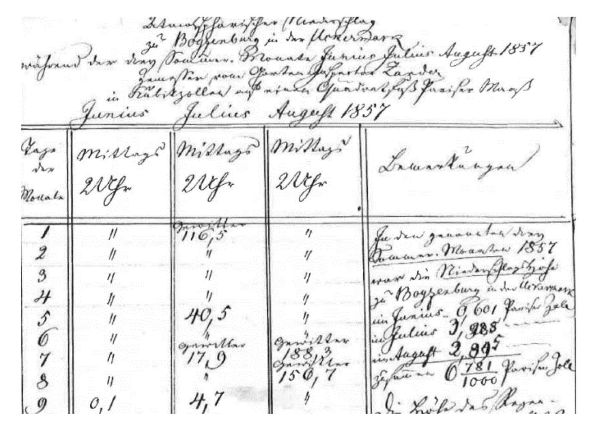
  57. Paalzow, Mr. Atmospheric Precipitation to Prenzlow in the Uckermark during the three summer months June, July, August 1857; measured by Mr. Mangelsdorf, Weise, and Zander. Available in the Brandenburg State Archive. 1857.
Figure 1. Overview of climate stations, (a) stations with less than two missing trend values between 1901 and 2019 (small rectangles), stations for a more detailed analysis (large rectangles), and stations with high-resolution data (dots), (b) the number of trend values per CLINO (Climate Normals) period.
Water 12 01950 g001
Figure 2. Distribution of Kendall’s tau for the CLINO periods with thresholds for heavy rainfall days in mm d−1. (a) all stations and (b) the 111 stations with 9–10 trend values. The lines represent the median as well as the 25% and 75% quantiles.
Water 12 01950 g002
Figure 3. Seasonal distribution of Kendall’s tau for the CLINO periods since 1901 and thresholds in mm d−1, 111 stations, (a) summer, and (b) winter. A similar pattern for all stations (1951–2019). The lines represent the median as well as the 25% and 75% quantiles.
Water 12 01950 g003
Figure 4. The difference in strength and direction of Kendall’s tau between nearby stations, over all available CLINO periods.
Water 12 01950 g004
Figure 5. The strength and direction of Kendall’s tau derived from daily sums starting at 6:00 UTC compared to 8:00 UTC.
Water 12 01950 g005
Figure 6. Increasing (red) and decreasing (blue) trends of heavy rainfall days with ≥20 mm at rainfall stations, for years (y), summer (s), and winter (w). For the sake of readability, the maps show only the active stations and four CLINO periods.
Water 12 01950 g006
Figure 7. Dominantly increasing (red) and decreasing (blue) trends of heavy rainfall days in German natural regions, for different thresholds (rows), seasons (columns), and periods (color), (cf. Table A2 in Appendix B).
Water 12 01950 g007
Figure 8. Heavy rainfall days with ≥20 mm and trend at the lowland station Lindenberg.
Water 12 01950 g008
Figure 9. Frequency of rainfall days with ≥20 mm and trend at station Wendelstein (1951–2012), elevation changed from 1735 m to 1832 m a.s.l. (above sea level) in March 1963.
Water 12 01950 g009
Figure 10. Frequency of rainfall days with ≥20 mm and trend at station Zugspitze (1951–2012, similar to Figure 9).
Water 12 01950 g010
Figure 11. Frequency of rainfall days with ≥20 mm and trend at station Zugspitze (1901–2019, full time-series).
Water 12 01950 g011
Figure 12. Heavy rainfall days with ≥20 mm and trends at Hohenpeißenberg, Alpine foothills, location changes in 1940 and 1948.
Water 12 01950 g012
Figure 13. Frequency of rainfall events compared to three 24 h sums (0:00 UTC, 06:00 UTC, and 07:30 UTC) at Müncheberg, thresholds ≥20 mm/event, and 20 mm d−1.
Water 12 01950 g013
Figure 14. Rainfall erosivity in Müncheberg, with linear trends for 1955–2019 and 1991–2019. EI30 values for April–October. Long-term mean value in yellow.
Water 12 01950 g014
Figure 15. The thunderstorm on 5 June 2007 in North-East (NE) Germany and its effect on the rainfall erosivity. (a) The arrow indicates its route. The rainfall intensity increases from blue to purple (above) and from blue to orange (inset map), data sources: WetterOnline and rain radar data of the DWD, (b) annual rainfall erosivity for the stations Dedelow (Ded, dark blue) and Grünow (GR, light blue), about 95 km north of Müncheberg in NE Germany (long-term mean values in yellow), data source: 10min-data ZALF for Dedelow; DWD for Grünow.
Water 12 01950 g015
Figure 16. Hand-written protocol (in Sütterlin letters) of rainfall depths. The columns indicate the day of the month at months June, July, and August 1857 and the amount of rainfall at 2 pm [57].
Water 12 01950 g016
Table 1. Summary of stations with calculated trend values.
ValueStations with 9–10 Trend ValuesOther Stations
Total number111 14552
Shifts since instalment2.31.9
Stations without shifts222450
Distance (m), weighted mean 2405263
Elevation (m), absolute change, weighted mean3.22.7
1 Shown in Figure 1, 2 time-weighted, includes the period of the original position, 0 m for stable stations.
Table 2. Combinations of CLINO (Climate Normals) period and threshold with significantly different trends for stable and shifted stations in Germany.
CLINO PeriodThreshold in mm d−1
1921–195010, 20, 30
1961–199030
1981–201010, 20

