Changing River Flood Timing in the Northeastern and Upper Midwest United States: Weakening of Seasonality over Time?

Abstract

Climate change is likely to impact precipitation as well as snow accumulation and melt in the Northeastern and Upper Midwest United States, ultimately affecting the quantity and seasonal distribution of streamflow. The objective of this study is to analyze seasonality of long-term daily annual maximum streamflow (AMF) records and its changes for 158 sites in Northeastern and Upper Midwest Unites States. A comprehensive circular statistical approach comprising a kernel density method was used to assess the seasonality of AMF. Temporal changes were analyzed by separating the AMF records into two 30-year sub-periods (1951–1980 and 1981–2010). Results for temporal change in seasonality showed mixed pattern/trend across the stations. While for majority of stations, the distribution of AMF timing is strongly unimodal (concentrated around spring season) for the period 1951–1980, the seasonal modes have weakened during the period 1981–2010 for several stations along the coastal region with simultaneous emergence of multiple modes indicating changes of seasonality therein. The fresh statistical approach based on non-parametric circular density estimates reduces some of the limitations of previous studies to detect and model event timing distributions with multiple seasons and addresses issues of non-stationarity in the data records of extreme events.

1. Introduction

Floods have generally been recognized as a stationary, independent and identically distributed random process by hydrologists [1]. However, in the recent decade, an increasing number of researchers are challenging the stationarity assumption in streamflow records [1,2,3]. Non-stationarity in streamflow characteristics may arise due to trends (because of natural climate variability or cyclical oscillations such as, El Niño), as well as alterations within Earth systems (due to anthropogenic influences) [1]. However, climate is the most important driver of changes in the hydrological cycle and particularly in river discharge since the climate system and water cycle are closely linked and any change in the climate system may induce changes in the hydrological cycle [4,5]. Shifts in climate could, therefore, result in: (i) increases or decreases in streamflow magnitudes and frequency [5]; (ii) changes in the timing of streamflow [6].

Numerous studies have examined temporal trends in streamflow magnitude and frequency across the continental United States [7,8,9,10,11,12,13]. Most of these studies have summarized that a significant change has been detected in low to moderate streamflow in many regions, while change in highflows are less significant [13,14]. While the magnitude and frequency of flood events is a primary concern for the sizing of stormwater sewers, flood protection, and other drainage appurtenances, it is the timing (or seasonality) of these events that critically impacts planning, maintenance schedules, and repairs. Similarly, agricultural practices, water and energy demands, and reservoir operation decisions are usually tied to the expected seasonal cycle of streamflows [15]. Hence, information on seasonality of flood events and its potential changes over time is crucial for water resource system planners and designers in developing strategies to reduce the impacts of climate change [16]. Despite the importance of seasonality of flood events and its potential changes over time for water resources management, there are limited studies related to the comprehensive characterization of the seasonality of flood events and its potential changes over time [17].

A useful basis for assessing the seasonality of flood events is circular statistics [18]. One major advantage of the use of circular statistics instead of linear statistics on the timing of flood events is its ability to provide an improved understanding of variables modeled as circular random processes (for example, the timing of an event within a cycle). Several studies have used a circular statistical approach for assessing the seasonality of flood events [5,17,18,19,20,21,22,23,24]. The majority of these studies have used two summary statistics based on mean and variability for analysis of timing of flood events. However, for catchments with bimodal or multimodal seasonality patterns, information from two summary statistics could be incomplete and ambiguous as shown by Dhakal et al. [25]. Furthermore, as an average statistic, the mean date may not reflect potential shifts in flood generation regime in a changing environment [23]. Few recent studies have attempted to address the limitations of the two summary statistics on seasonality characterization of flood events by using different approaches. For example, Villarini [17] examined the seasonality of annual maximum flows across the continental United States by using circular uniform, reflective symmetric and asymmetric distributions. Using a probabilistic method, Collins [24] characterized the multimodality of flood seasons for 90 Northeast U.S. watersheds and evaluated whether flood seasons have shifted earlier or later in the annual cycle. A recent study by Rutkowska et al. [18] made a notable contribution to this topic by using circular mixture distribution to model the date of maximum river flow in three catchments and properly reflect the sample multimodality. However, none of these studies has specifically explored if the temporal changes/shifts in seasonality have been caused by either weakening, strengthening, emergence or weathering of distributional modes of timing of flood events during different seasons or combination of two or more of these phenomena.

Given the limitations noted above, in this study we used a comprehensive method including a robust probabilistic approach based on non-parametric circular density estimates for the assessment of temporal changes in the calendar dates for annual maximum flows (AMF) in the Northeastern and Upper Midwest United States. Northeastern (NE) and Upper Midwest (MW) United States is known to experience a very diverse climate and a tremendous variety of weather systems [26]. Several studies have investigated the trends in streamflow for the Northeast U.S. and found that the magnitude of AMF in the NE has not increased in the 20th century [8,9,27,28]. However, positive trends in the number of high-frequency floods have been found in most New England rivers throughout the 20th and early 21st centuries with a steep increase around 1970 [29]. There are a limited number of studies related to the characterization of the seasonality of flood events and its potential changes over time for the NE and MW. Earlier winter-spring flows in the range of 7–14 days have been observed in the NE [30] and are thought to be linked to increased snow melting and rain-on-snow episodes [31], and this trend is likely to continue during the 21st century [6]. Villarini [17] and Ye et al. [23] found a strong seasonality in flooding across the continental United States including NE and MW. More recently, using peaks-over-threshold flood records over the period of 1941 to 2013, Collins [24] showed that the annual timing of flood-rich seasons for NE has generally not shifted earlier or later over the period of record. The main objective of our work is to identify the seasonality of AMF for the NE and MW region with greater accuracy and detail than previously available. More specifically, the goals of this study are to: (1) precisely explore whether the seasonality of AMF is multimodal for the NE and MW region; and (2) investigate whether there have been temporal shifts (non-stationarity) in the seasonality of the AMF across the region, and if yes, whether the temporal shifts have been caused by either weakening, strengthening, emergence or weathering of distributional modes of timing of AMF during different seasons. Results from this study can be helpful in disaster risk management [26] as well as in identifying changes in flood-generating mechanisms [23].

2. Materials and Methods

2.1. Data and Study Area

Our study area includes the 22 U.S. states east of the −98° W meridian and north of 36° N latitude NE–MW region [32]. Basins with near-natural conditions were selected from the USGS Geospatial Attributes of Gages for Evaluating Streamflow (Gauges II) dataset [32,33]. As a quality control, basins meeting the following two criteria were selected: (a) percentage of missing values (daily record) less than 20% per year, and (b) record length greater than or equal to 55 years. From the pool of available basins, 158 basins with drainage areas ranging between 10 and 2500 km² (average 1000 km²) met the two criteria (Figure S1). Missing data for the basins meeting the two quality control criteria were omitted and analyses conducted on the remaining data. Daily AMF from 158 basins for the period 1951–2010 (60 years) were extracted for analysis.

2.2. Statistical Methods

2.2.1. Circular Statistics

We used a method based on circular statistics [34,35] to evaluate seasonality. For the circular statistical method, calendar dates of AMF were converted to Julian dates (D), where D = 1 for January 1 and D = 365 (or 366 for leap year) for December 31. Following Dhakal et al. [25], the angular value (θ_i) representing the position for the date “D_i” in a unit circle was then computed using the formula:

$${\theta }_i=D_i\left(\frac{2\pi }{365}\right)$$

(1)

For a basin having “n” events, the mean direction parameter,$\overline{\theta }$, representing the mean date of occurrence of AMF was obtained by using the following relationships:

$$\overline{x}=\frac{{{\displaystyle \sum }}_{i=1}^n\cos \left({\theta }_i\right)}{n}$$

(2)

$$\overline{y}=\frac{{{\displaystyle \sum }}_{i=1}^n\sin ({\theta }_i)}{n}$$

(3)

$$\overline{\theta }={\tan }^{-1}\left(\frac{\overline{y}}{\overline{x}}\right)$$

(4)

where $\overline{x}$ and $\overline{y}$ represent the x- and y-coordinates of the mean date.

A length parameter measuring variability (dispersion) of n event occurrences about the mean date was obtained by using:

$$\rho =\frac{\sqrt{{\overline{x}}^2+{\overline{y}}^2}}{n}$$

(5)

The parameter, ρ, ranges from 0 to 1; a value of 0 would indicate that the AMF events are distributed uniformly around the year and a value of 1 would indicate that all events occurred on the same day of the year. Several other studies [5,17,19,20,21,22,23] have used two summary statistics based on mean (Equation (4)) and variability (Equation (5)) for analysis of streamflow records. For analysis of potential shifts in seasonality of AMF, we divided the data records into two sub-periods, 1951–1980 and 1981–2010, and computed difference in mean and variability of AMF for each basin. The significance of changes in the mean and variability of AMF dates were determined by using the bootstrap resampling approach. For each basin, 2 random blocks of equal size (30 years) were generated from the AMF dataset using the bootstrap method and 1000 estimates of difference in circular mean and variability were generated. The mean (spread) of AMF was assumed to have shifted at the 95% confidence level, if the difference was outside of the 5th and 95th percentile of the bootstrap estimates. In addition to the measure of circular mean and variability, we also used the Rao Spacing test [34,35], a non-parametric statistical test based on the sample arc length to check a null hypothesis of no seasonal preference (“no seasonality”) in AMF dates.

2.2.2. Circular Distribution Function

The total probability of a circular distribution is concentrated on the circumference of a unit circle [35]. The von Mises distribution, which is often used to model circular data, has the probability density function (PDF):

$$f\left(\theta ;\mathsf{\mu },\kappa \right)=\frac{1}{2\pi I_0\left(\kappa \right)}{e}^{kcos\left(\theta -\mathsf{\mu }\right)},0\le \theta <2\pi$$

(6)

where θ is a mean direction parameter, and κ ≥ 0 is a concentration parameter. I₀ (κ) in the normalizing constant is the modified Bessel function of the first kind of order 0 [35]. The parameter, κ, is the smoothing parameter or bandwidth that determines the concentration of θ values towards the mean direction µ. We estimated the global optimum bandwidth as the median of the 1000 sets of bandwidths, estimated for the entire period using the likelihood cross-validation (LCV) method, which selects a bandwidth maximizing the likelihood cross-validation function [36]. The LCV method is selected since it produces reasonable bandwidth values for multimodal distributions [36]. Non-parametric bootstrap method was used to evaluate the significance of the probability density estimates. The bootstrap generates new samples by drawing at random with replacement from the original sample. Point-by-point estimate of variability was compared against assumed uniform distribution obtained from resampled data (n = 1000). An example of circular density estimates of the AMF dates has been presented in Figure 1 for Blockhouse Creek near the English Center in Pennsylvania. In Figure 1, the individual AMF dates are plotted as black dots along the perimeter of the inner circle and the irregular solid black line represents the circular density estimates of the AMF dates. It must be noted that the unit circle begins at (x, y) of (1.0, 0.0), and goes counterclockwise in a 360 degree circle. The height of the rose diagram or circular histogram presented in Figure 1 shows the number of maxima occurring in a calendar date. The dotted line represents median estimate for significance based on density estimates using resampled data (n = 1000). Each of our resampled data comprise a uniform distribution with no seasonality. For Blockhouse Creek, the circular distribution appears to be unimodal with significant density spanning though January–April period. R statistical package “circular” [37] was used to execute computations. A robust framework on the circular statistical approach was developed by Dhakal et al. [25] to explore the extreme precipitation seasonality for 10 stations in Maine.

3. Results

3.1. Spatial Pattern of Seasonality Based on Circular Mean and Variability

The spatial pattern of seasonality of AMF based on mean ($\overline{\theta }$) and variability (ρ) is presented in Figure 2. Here the direction of arrows indicates the mean, and the length of arrows indicate the variability or strength of seasonality. The frequency (number) of stations with similar mean streamflow seasonality is presented in Figure 2a. Figure 2a shows that majority of stations have their maxima mostly in the months of February, March and April; few stations have their maxima in the months of January and May. The results for $\overline{\theta }$ and ρ are consistent with studies by Villarini [17] and Ye et al. [23]. Figure 2 reveals that for the study area, west and northeast regions have relatively strong seasonality as compared to southeast region. According to Ye et al. [23], pattern of seasonality observed in the west and northeast regions is likely related to the antecedent soil water storage accumulating from winter to spring. On the other hand, comparatively weak seasonality in the southeast region might be related to multimodal seasonality of AMF arising from a mixture of causative mechanisms [38]. As stated by Hirschboeck [39], the regional patterns of seasonal weather and atmospheric moisture pathways is regulated by the large-scale, general circulation of the atmosphere and it causes the multimodality in the probability distribution of flood seasonality.

3.1.1. Temporal Change in Seasonality

For analysis of potential shifts in flood seasonality, we divided the data records into two 30-year sub-periods, 1951–1980 and 1981–2010. The spatial pattern of difference (earlier–later) in circular mean ($\overline{\theta }$) and variability (ρ) is presented in Figure 3a,b respectively. Mixed results were obtained for the difference in mean; 85 stations showing decrease in mean (indicating that AMF date has shifted earlier) and 73 stations showing increase in mean (indicating that AMF date has shifted later). For 15 stations, AMF date was significantly earlier for the latest time period (1981–2010) as compared to the earlier time period (1951–1980) and most of these stations are concentrated in the northeastern region of the study area. On the other hand, for 14 stations, AMF date was significantly later for the latest time period and although the stations with such seasonality pattern are spread throughout, the majority are concentrated in southeast region. The results for the difference in circular variability (Figure 3b) is interesting and more spatially coherent as compared to the difference in mean. For 116 stations the difference in variability (earlier–later) is positive (indicating the weakening of seasonality for the latest time period) and for 42 stations, the difference in variability is negative (indicating the strengthening of seasonality for the latest time period). For 47 stations, the positive difference in variability is significant and most of these stations are in the eastern half of the study area mainly along the coastal states. On the other hand, for only 6 stations, the negative difference in variability is significant and most of the stations (5 out of 6) are concentrated in the southeastern region of the study area.

To further explore our results from Figure 3, we extracted the frequency of stations with similar mean and variability and plotted the results in Supplementary Figure S2. Figure S2a,c show the frequency of stations with similar mean and variability of seasonality for the earlier period, while Figure S2b,d show the frequency of stations with similar mean and variability of seasonality for the latest period. Comparing Figure S2a,b it can be seen that majority of stations have their maxima mostly in the months of February, March and April for both time periods. However, comparing Figure S2c,d, it can be seen that the frequency of the stations with weaker seasonality (smaller values of ρ) has increased for the recent period. As noted earlier, this might have been caused by either weakening, strengthening, emergence or weathering of seasonality modes during different seasons. Some of these phenomena might result in the bimodal or multimodal flood seasonality patterns.

In addition to the estimation of changes in mean and variability, we also conducted a Rao spacing test to check the null hypothesis of uniformity on AMF dates for earlier and latest time periods separately and presented our results in Figure 4. Figure 4a shows the uniformity test results based on the earlier period (1951–1980) and Figure 4b shows the uniformity test results based on the latest period (1981–2010). For 43 stations, the null hypothesis of uniformity was accepted for the earlier period, while for 81 stations, the null hypothesis of uniformity was accepted for the latest time period. Majority of the stations accepting the null hypothesis of uniformity (showing no seasonality) is in the southern region of the study area, particularly concentrated on the southern coastal states. As expected, these are the stations showing the positive difference in variability (indicating the weakening of seasonality for the latest time period) in Figure 3b. As shown by Dhakal et al. [25], in many cases when the distribution is multimodal, the uniformity test does not capture the true/actual distribution. This means that for many stations for which the null hypothesis of uniformity is accepted, the distribution might be multimodal instead of uniform. To sum up, methods based on two summary statistics, and a uniformity test, provided some useful insight regarding the distribution of AMF dates. However, for stations with complex (multimodal) seasonality pattern, results from either two summary statistics or uniformity test might be incomplete and even misleading in many cases. To this end, we used a circular density method that can capture the diversity of distribution types, including multimodality and results are presented in the next section.

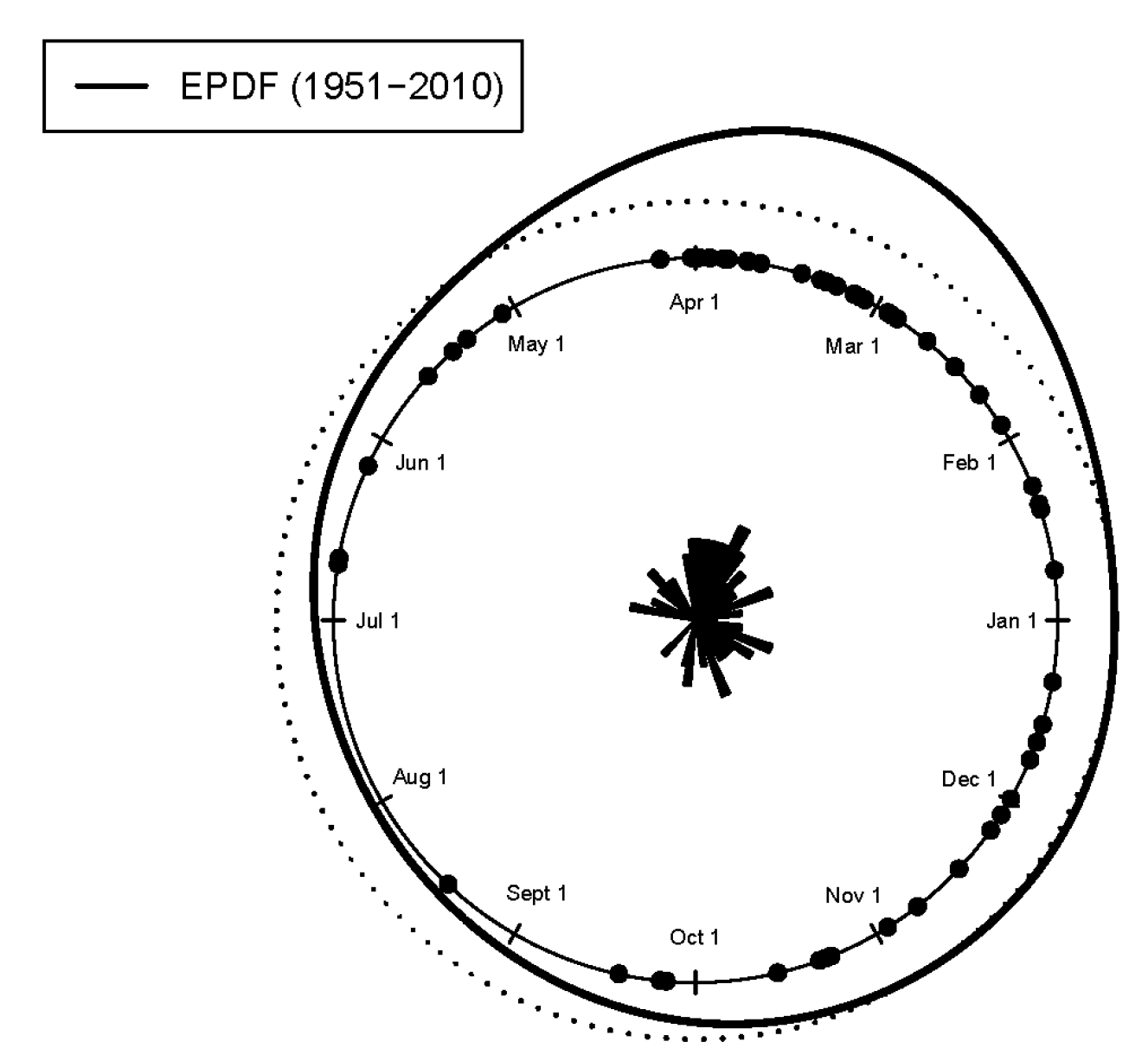
3.2. Seasonality Based on Circular Density Method

As noted earlier, for analysis of potential shifts in seasonality of AMF, we divided the data records into two sub-periods, 1951–1980 and 1981–2010. Kernel circular density was computed for each station based on the calendar dates of AMF for the earlier period and latest period separately. To assess the significance of the density estimates, the bootstrap technique was used as explained in Section 2.2. A median estimate was obtained from the ensemble of distributions resulting from bootstrap resampling (n = 1000). For each sub-period, point-by-point estimate of variability was compared against assumed uniform distribution obtained from resampled data. In general, we have identified four different cases of changes in seasonal modes for AMF dates; (i) weakening of seasonality, (ii) strengthening of seasonality, (iii) unimodal and strong seasonality for both the earlier and latest time periods, (iv) uniform or no preferred seasonality for both the earlier and latest time periods. An example of these four cases of changes in seasonal modes for AMF has been presented in Figure 5. Figure 5a displays the case of weakening of seasonal modes over time for the Hubbard River near West Hartland in Connecticut. Black and grey lines represent the density estimates for the periods 1951–1980 and 1981–2010, respectively, and the dotted line represents a 95% estimate of significance (uncertainty) from bootstrap resampling. The distribution of seasonality for 1951–1980 exhibit unimodal pattern with significant mode congregated in winter and spring seasons (February–May). On the other hand, for 1981–2010, the distribution exhibit trimodal pattern with the recent weakening of the winter and spring mode and simultaneous emergence of significant modes during summer season (May–June), and fall season (September–December). Figure 5b displays the case of strengthening of seasonal modes over time for the Rapid Creek near Iowa City in Iowa. The distribution of seasonality for 1951–1980 exhibits a bi-modal pattern with one significant mode centered in February–March period, and the other significant mode centered in the May–July period. On the other hand, for 1981–2010, the distribution exhibits a bi-modal pattern with the recent strengthening of the May–July period mode. Figure 5c displays the case of no change in seasonal modes over time with strong unimodal seasonality for Blockhouse Creek near the English Center in Pennsylvania. The distribution of seasonality for both the earlier and latest time periods exhibits unimodal pattern with significant mode congregated in winter and spring seasons (February–April). Figure 5d displays the case of more or less uniform distribution of AMF dates for S F Quantico Creek near Independent Hill in Virginia; this case represents no preferred seasonality for both time periods (hence no change in seasonal modes).

Similar to above analysis, kernel circular density estimates were obtained for all 158 stations for each time period separately. To spatially visualize the stations showing the changes in seasonal modes for AMF dates (similar to cases like those presented in Figure 5a,b, we extracted the stations with significant and unique seasonal modes (no overlapping significant density estimates between two time periods) corresponding to each month of the year. A station showing unique seasonal mode for the latest time period represents the case where the seasonal mode has weakened over time such as the case in Figure 5a. Similarly, a station showing unique seasonal mode for the earlier period represents the case where the seasonal mode has strengthened over time such as the case in Figure 5b. Figure 6a displays the spatial pattern of stations with unique seasonal mode for spring season (March–May) for the earlier period and Figure 6b displays the spatial pattern of stations with unique seasonal mode for spring season (March–May) for the latest period. It can be seen that for spring season the number of stations with unique seasonal mode has increased by 118% for the latest time period, with the majority of stations showing the unique seasonal mode for the month of May and located in the southeastern coastal region of the study area. Figure 6c displays the spatial pattern of stations with a unique seasonal mode for the summer season (June–August) for the earlier period and Figure 6d displays the spatial pattern of stations with a unique seasonal mode for the summer season for the latest period. It can be seen that for summer season the number of stations with a unique seasonal mode has increased by 144% for the latest time period, with majority of stations showing the unique seasonal mode for the months of June and July and located in the southern region (both coastal and inland) of the study area. Figure 6e displays the spatial pattern of stations with a unique seasonal mode for fall season (September–November) for the earlier period and Figure 6f displays the spatial pattern of stations with a unique seasonal mode for fall season for the latest period. It can be seen that for fall season the number of stations with a unique seasonal mode has increased by 70% for the latest time period, with majority of stations showing the unique seasonal mode for the month of November and located along the coastal sites in the eastern region of the study area. Figure 6g displays the spatial pattern of stations with a unique seasonal mode for winter season (December–February) for the earlier period and Figure 6h displays the spatial pattern of stations with a unique seasonal mode for winter season for the latest period. It can be seen that for winter season the number of stations with a unique seasonal mode has increased by 45% for the latest time period, with majority of stations showing unique seasonal modes for the months of December and January. It is interesting to see that for winter season, the unique seasonal modes appeared at many inland sites of the southern region of the study area.

The results presented in Figure 6 supported as well as augmented our results based on two summary statistics, and a uniformity test presented in Section 3.1.1. To sum up, our analysis showed that seasonality has weakened over time for many sites for NE and MW region and most of that weakening was observed in the coastal sites. In other words, there is emergence of significant modes in AMF seasonality for these locations during the latest time period. The reason for the emergence of modes during the month of November along the coastal sites might be due to the increase in the heavy precipitation trends associated with tropical cyclones in the North Atlantic basins over the last 30 years [26,40,41,42,43]. Similarly, the emergence of modes during the months of May and early June might be due to the emergence of extreme precipitation seasonality modes during late spring and early summer season for the recent time period as shown by Dhakal et al. [25]. Detailed exploration of the potential physical mechanisms for these changes is beyond the scope of this study.

4. Conclusions and Discussion

This study builds on earlier studies by providing a detailed assessment of seasonality of daily annual maximum streamflow (AMF) events for the Northeastern and Upper Midwest United States. Circular statistical methodologies are used to understand the seasonality of flood events, as well as the recent changes for 158 stations. The main findings of the paper are summarized as follows:

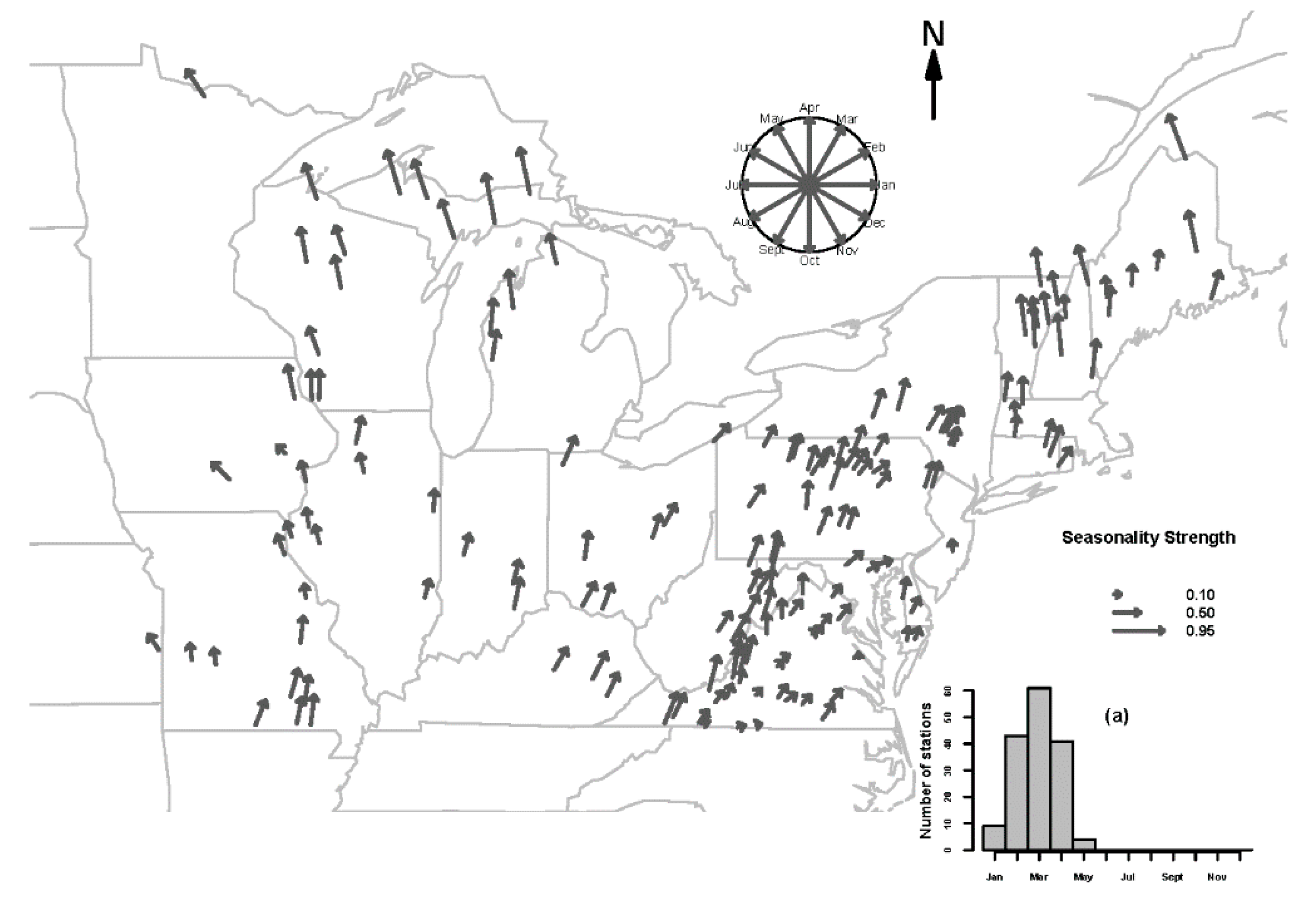
• Assessment of spatial patterns of seasonality for the last six decades (1951–2010) based on the mean date and variability in the occurrence of the extreme events shows strong seasonality of the AMF. Majority of stations have their maxima mostly in the months of February, March and April.
• Comparing the AMF seasonality before and after 1980 (using two 30-year sub-periods, 1951–1980 and 1981–2010) based on changes in the mean date and variability as well using Rao spacing test, a nonparametric uniformity test, shows that majority of stations have no significant change in their mean date with their maxima mostly in the months of February, March and April for both the time periods. However, for the recent sub-period, the seasonality has weakened for several sites indicated by the lower values of variability and higher number of stations accepting the null hypothesis of uniformity.
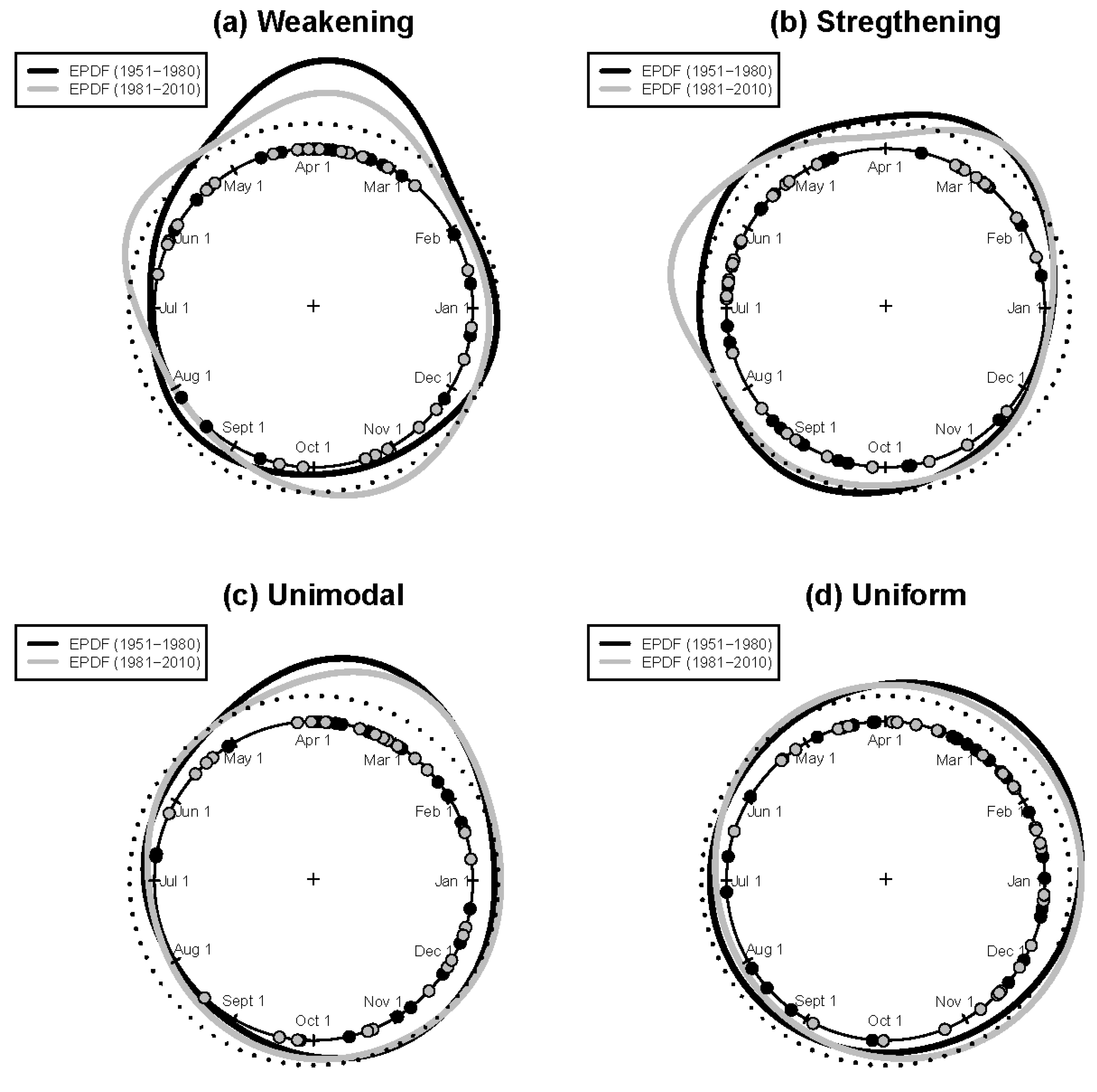
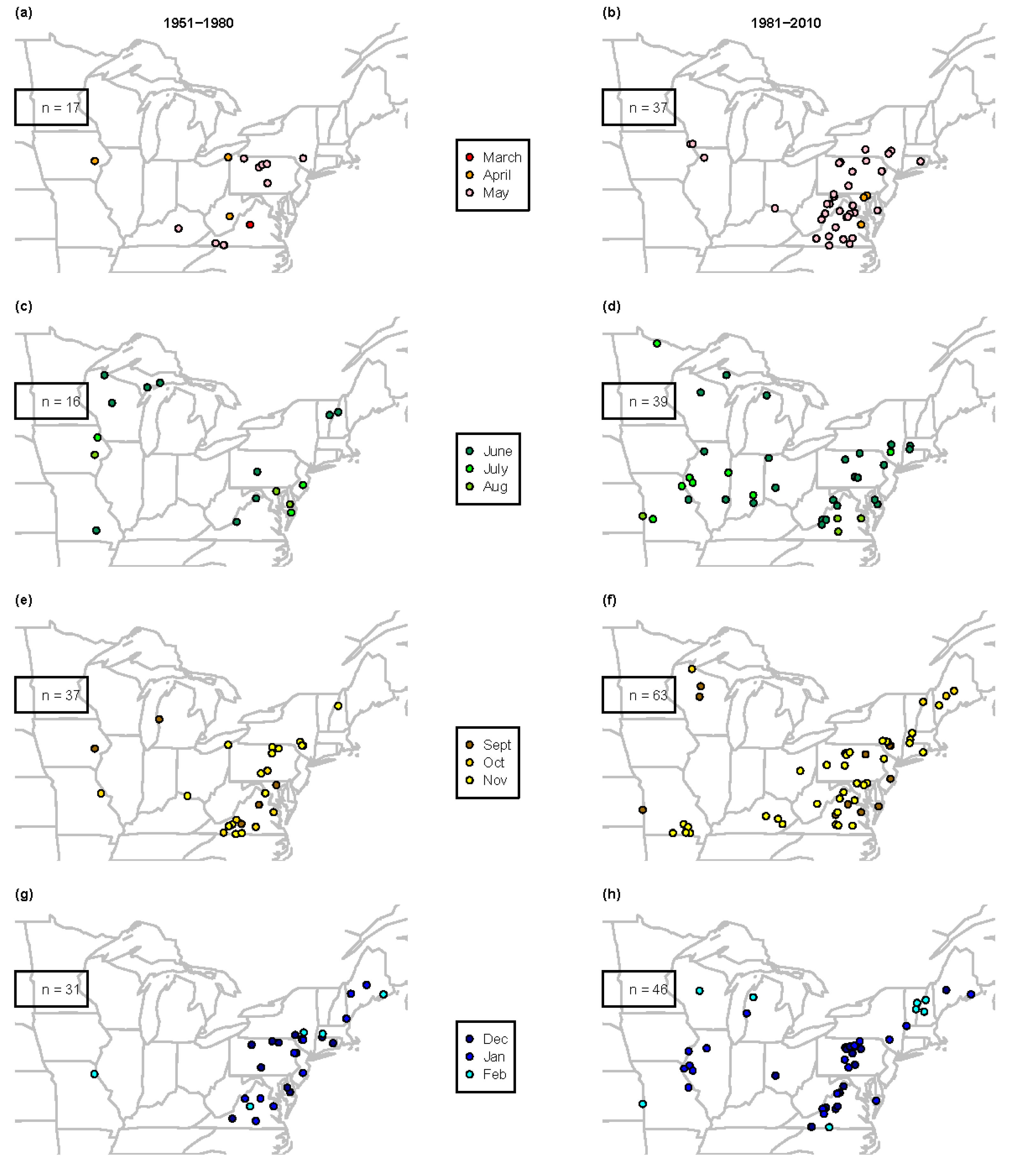
• Using the non-parametric circular density approach, four different cases of seasonality change over time for AMF dates were identified in this study: (i) weakening of seasonality, (ii) strengthening of seasonality, (iii) unimodal and strong seasonality for both the earlier and latest time period, (iv) uniform or no preferred seasonality for both the earlier and latest time period. Assessment of temporal change in seasonality of the AMF based on non-parametric circular density estimates shows that for the majority of stations significant density estimates are observed during the months of February, March and April for both time periods. In addition to this, it was observed that seasonal modes of AMF dates have weakened over time for a number of sites along the coastal region with the emergence of significant modes during late spring and early summer (May–June) as well as fall season (mid-September–November). The reason for the emergence of seasonality modes during the month of November along the coastal sites might be due to an increase in the heavy precipitation trends associated with tropical cyclones in the North Atlantic basins over the last 30 years [26,40,41,42,43]. Similarly, the emergence of modes during the months of May and early June might be due to the emergence of extreme precipitation seasonality modes during late spring and early summer season for the latest time period as shown by Dhakal et al. [25].

Flood events put communities through “stress tests.” Our study focused on the seasonality of AMF has important implications for flood management and mitigation. For example, changes in seasonality of AMF provides an opportunity to re-examine the timing of seasonality-dependent decisions about the repair and maintenance of flood controlling infrastructures such as decisions appertaining to stormwater management [25]. Additionally, fresh statistical approach based on nonparametric circular density estimates reduces some of the limitations of trend analysis of previous studies to detect and model event timing distributions with multiple seasons and address issues of non-stationarity in the data records of extreme events.

Seasonality based on historic data can only reveal what has happened in the past in terms of important dimensions of the extreme flow regime [16]. A more comprehensive view of the present and possible future extreme conditions can be obtained by combining trend analysis of historical data with analysis of data obtained from modelling climate change projections using downscaled results from Global Climate Models (GCMs) along with an appropriate hydrological model [16]. Our continuing work aims to use the proposed approach for seasonality analysis on historical data as well as analysis on data from GCM-based climate projections to regional and global scales.

References

1. Jain, S.; Lall, U. Magnitude and timing of annual maximum floods: Trends and large-scale climatic associations for the Blacksmith Fork River, Utah. Water Resour. Res. 2000, 36, 3641–3651. [Google Scholar] [CrossRef]
2. Jain, S.; Lall, U. Floods in a changing climate: Does the past represent the future? Water Resour. Res. 2001, 37, 3193–3205. [Google Scholar] [CrossRef]
3. Milly, P.C.D.; Betancourt, J.; Falkenmark, M.; Hirsch, R.M.; Kundzewicz, Z.W.; Lettenmaier, D.P.; Stouffer, R.J. Stationarity is dead: Whither water management? Science 2008, 319, 573–574. [Google Scholar] [CrossRef] [PubMed]
4. Ehsanzadeh, E.; Adamowski, K. Trends in timing of low stream flows in Canada: Impact of autocorrelation and long-term persistence. Hydrol. Process. 2010, 24, 970–980. [Google Scholar] [CrossRef]
5. Bloschl, G.; Hall, J.; Parajka, J.; Perdigao, R.A.P.; Merz, B.; Arheimer, B.; Aronica, G.T.; Bilibashi, A.; Bonacci, O.; Borga, M.; et al. Changing climate shifts timing of European floods. Science 2017, 357, 588–590. [Google Scholar] [CrossRef] [PubMed] [Green Version]
6. Campbell, J.L.; Driscoll, C.T.; Pourmokhtarian, A.; Hayhoe, K. Streamflow responses to past and projected future changes in climate at the Hubbard Brook Experimental Forest, New Hampshire, United States. Water Resour. Res. 2011, 47, W02514. [Google Scholar] [CrossRef]
7. Lettenmaier, D.P.; Wood, E.F.; Wallis, J.R. Hydro-climatological trends in the continental United States, 1948–1988. J. Clim. 1994, 7, 586–607. [Google Scholar] [CrossRef] [Green Version]
8. Lins, H.F.; Slack, J.R. Streamflow trends in the United States. Geophys. Res. Lett. 1999, 26, 227–230. [Google Scholar] [CrossRef] [Green Version]
9. Douglas, E.M.; Vogel, R.M.; Kroll, C.N. Trends in floods and low flows in the United States: Impact of spatial correlation. J. Hydrol. 2000, 240, 90–105. [Google Scholar] [CrossRef]
10. Groisman, P.Y.; Knight, R.W.; Karl, T.R. Heavy precipitation and high streamflow in the contiguous United States: Trends in the twentieth century. Bull. Am. Meteorol. Soc. 2001, 82, 219–246. [Google Scholar] [CrossRef] [Green Version]
11. Small, D.; Islam, S.; Vogel, R.M. Trends in precipitation and streamflow in the eastern US: Paradox or perception? Geophys. Res. Lett. 2006, 33. [Google Scholar] [CrossRef]
12. Kalra, A.; Piechota, T.C.; Davies, R.; Tootle, G.A. Changes in US streamflow and western US snowpack. J. Hydrol. Eng. 2008, 13, 156–163. [Google Scholar] [CrossRef]
13. Ahn, K.H.; Palmer, R.N. Trend and variability in observed hydrological extremes in the United States. J. Hydrol. Eng. 2015, 21, 04015061. [Google Scholar] [CrossRef]
14. McCabe, G.J.; Wolock, D.M. A step increase in streamflow in the conterminous United States. Geophys. Res. Lett. 2002, 29, 2185. [Google Scholar] [CrossRef]
15. Baldwin, C.K.; Lall, U. Seasonality of streamflow: The upper Mississippi River. Water Resour. Res. 1999, 35, 1143–1154. [Google Scholar] [CrossRef]
16. Burn, D.H.; Sharif, M.; Zhang, K. Detection of trends in hydrological extremes for Canadian watersheds. Hydrol. Process. 2010, 24, 1781–1790. [Google Scholar] [CrossRef]
17. Villarini, G. On the seasonality of flooding across the continental United States. Adv. Water Resour. 2016, 87, 80–91. [Google Scholar] [CrossRef] [Green Version]
18. Rutkowska, A.; Kohnová, S.; Banasik, K. Probabilistic Properties of the Date of Maximum River Flow, an Approach Based on Circular Statistics in Lowland, Highland and Mountainous Catchment. Acta Geophys. 2018, 66, 755–768. [Google Scholar] [CrossRef] [Green Version]
19. Bayliss, A.C.; Jones, R.C. Peaks-Over-Threshold Flood Database; Institute of Hydrology: Wallingford, UK, 1993. [Google Scholar]
20. Burn, D.H. Catchment similarity for regional flood frequency analysis using seasonality measures. J. Hydrol. 1997, 202, 212–230. [Google Scholar] [CrossRef]
21. Parajka, J.; Kohnová, S.; Merz, R.; Szolgay, J.; Hlavčová, K.; Blöschl, G. Comparative analysis of the seasonality of hydrological characteristics in Slovakia and Austria. Hydrol. Sci. J. 2009, 54, 456–473. [Google Scholar] [CrossRef]
22. Parajka, J.; Kohnová, S.; Bálint, G.; Barbuc, M.; Borga, M.; Claps, P.; Blöschl, G. Seasonal characteristics of flood regimes across the Alpine–Carpathian range. J. Hydrol. 2010, 394, 78–89. [Google Scholar] [CrossRef] [PubMed]
23. Ye, S.; Li, H.Y.; Leung, L.R.; Guo, J.; Ran, Q.; Demissie, Y.; Sivapalan, M. Understanding flood seasonality and its temporal shifts within the contiguous United States. J. Hydrometeorol. 2017, 18, 1997–2009. [Google Scholar] [CrossRef]
24. Collins, M.J. River flood seasonality in the Northeast United States: Characterization and trends. Hydrol. Process. 2019, 33, 687–698. [Google Scholar] [CrossRef]
25. Dhakal, N.; Jain, S.; Gray, A.; Dandy, M.; Stancioff, E. Nonstationarity in seasonality of extreme precipitation: A nonparametric circular statistical approach and its application. Water Resour. Res. 2015, 51, 4499–4515. [Google Scholar] [CrossRef]
26. Dhakal, N. Changing impacts of North Atlantic tropical cyclones on extreme precipitation distribution across the Mid-Atlantic United States. Geosciences 2019, 9, 207. [Google Scholar] [CrossRef] [Green Version]
27. Lins, H.F.; Slack, J.R. Seasonal and regional characteristics of US streamflow trends in the United States from 1940 to 1999. Phys. Geogr. 2005, 26, 489–501. [Google Scholar] [CrossRef]
28. Villarini, G.; Smith, J.A. Flood peak distributions for the eastern United States. Water Resour. Res. 2010, 46, W06504. [Google Scholar] [CrossRef] [Green Version]
29. Armstrong, W.H.; Collins, M.J.; Snyder, N.P. Increased frequency of low-magnitude floods in New England. JAWRA J. Am. Water Resour. Assoc. 2012, 48, 306–320. [Google Scholar] [CrossRef]
30. Hodgkins, G.A.; Dudley, R.W.; Huntington, T.G. Changes in the timing of high river flows in New England over the 20th century. J. Hydrol. 2003, 278, 244–252. [Google Scholar] [CrossRef] [Green Version]
31. Hodgkins, G.A.; Dudley, R.W. Changes in late-winter snowpack depth, water equivalent, and density in Maine, 1926–2004. Hydrol. Process. 2006, 20, 741–751. [Google Scholar] [CrossRef]
32. Demaria, E.M.; Palmer, R.N.; Roundy, J.K. Regional climate change projections of streamflow characteristics in the Northeast and Midwest US. J. Hydrol. Reg. Stud. 2016, 5, 309–323. [Google Scholar] [CrossRef] [Green Version]
33. Falcone, J.D.; Carlisle, D.M.; Wolock, D.M.; Meador, M.R. GAGES: A stream gage database for evaluating natural and altered flow conditions in the conterminous United States. Ecology 2010, 91, 621. [Google Scholar] [CrossRef]
34. Mardia, K.V. Statistics of Directional Data; Academic Press: New York, NY, USA, 1972. [Google Scholar]
35. Jammalamadaka, S.R.; Sengupta, A. Topics in Circular Statistics; World Scientific: Singapore, 2001; Volume 5. [Google Scholar]
36. Oliveira, M.; Crujeiras, R.M.; Rodríguez-Casal, A. Nonparametric circular methods for exploring environmental data. Environ. Ecol. Stat. 2013, 20, 1–17. [Google Scholar] [CrossRef]
37. Agostinelli, C.; Lund, U. R Package ‘Circular’: Circular Statistics (Version 0.4–7). 2013. Available online: https://r-forge.r-project.org/projects/circular/ (accessed on 24 December 2019).
38. Hirschboeck, K.K. Hydroclimatically-Defined Mixed Distributions in Partial Duration Flood Series. In Hydrologic Frequency Modeling; Singh, V.P., Ed.; Reidel Publishing Company: Dordrecht, The Netherlands, 1987; pp. 199–212. [Google Scholar]
39. Hirschboeck, K.K. Climate and floods. Natl. Water Summ. 1988, 89, 67–88. [Google Scholar]
40. Lau, K.M.; Zhou, Y.P.; Wu, H.T. Have tropical cyclones been feeding more extreme rainfall? J. Geophys. Res. Atmos. 2008, 113. [Google Scholar] [CrossRef] [Green Version]
41. Kunkel, K.E.; Easterling, D.R.; Kristovich, D.A.; Gleason, B.; Stoecker, L.; Smith, R. Recent increases in US heavy precipitation associated with tropical cyclones. Geophys. Res. Lett. 2010, 37, 2–5. [Google Scholar] [CrossRef]
42. Barlow, M. Influence of hurricane-related activity on North American extreme precipitation. Geophys. Res. Lett. 2011, 38. [Google Scholar] [CrossRef]
43. Dhakal, N.; Jain, S. Nonstationary influence of the North Atlantic tropical cyclones on the spatio-temporal variability of the eastern United States precipitation extremes. Int. J. Climatol. 2019, 40, 3486–3499. [Google Scholar] [CrossRef]
Figure 1. Empirical probability density function (EPDF) estimates of the annual maximum streamflow dates for Blockhouse Creek near the English Center in Pennsylvania. The dotted line represents the median estimate for significance based on density estimates using resampled data (n = 1000).
Water 12 01951 g001
Figure 2. Spatial patterns of seasonality of daily annual maximum streamflow for the period 1951–2010 (n = 60) based on circular mean ( θ ¯ ) and variability (ρ); (a) the frequency of stations with similar mean streamflow seasonality. Here the direction of arrows indicates the mean and the length of arrows indicate the strength of seasonality.
Water 12 01951 g002
Figure 3. Spatial patterns of changes in seasonality based on circular mean and variability; (a) changes in mean annual maximum streamflow (AMF) dates, (b) changes in variability (spread) of the AMF dates. The asterisk (*) symbols represent the basins with significant changes.
Water 12 01951 g003
Figure 4. Spatial patterns of Rao spacing test results; a nonparametric statistical test to check the null hypothesis of uniformity of AMF dates for the periods; (a) 1951–1980; (b) 1981–2010.
Water 12 01951 g004
Figure 5. Four different cases of changes in seasonal modes for AMF dates identified based on circular density estimates; (a) weakening of seasonality for Hubbard River near West Hartland in Connecticut, (b) strengthening of seasonality for Rapid Creek near Iowa City in Iowa; (c) unimodal and strong seasonality for Blockhouse Creek near the English Center in Pennsylvania; (d) uniform or no preferred seasonality for S F Quantico Creek near Independent Hill in Virginia. Black and grey lines represent the density estimates for the periods 1951–1980 and 1981–2010 respectively, and the dotted line represents a 95% estimate of significance (uncertainty) from bootstrap resampling.
Water 12 01951 g005
Figure 6. Spatial patterns of stations with unique seasonal modes (no overlapping density estimates between two-time periods) corresponding to each month of the year for the period 1951–1980 (a,c,e,g) and 1981–2010 (b,d,f,h).
Water 12 01951 g006